Hardware Friendly Robust Synthetic Basis Feature Descriptor

Abstract

Finding corresponding image features between two images is often the first step for many computer vision algorithms. This paper introduces an improved synthetic basis feature descriptor algorithm that describes and compares image features in an efficient and discrete manner with rotation and scale invariance. It works by performing a number of similarity tests between the feature region surrounding the feature point and a predetermined number of synthetic basis images to generate a feature descriptor that uniquely describes the feature region. Features in two images are matched by comparing their descriptors. By only storing the similarity of the feature region to each synthetic basis image, the overall storage size is greatly reduced. In short, this new binary feature descriptor is designed to provide high feature matching accuracy with computational simplicity, relatively low resource usage, and a hardware friendly design for real-time vision applications. Experimental results show that our algorithm produces higher precision rates and larger number of correct matches than the original version and other mainstream algorithms and is a good alternative for common computer vision applications. Two applications that often have to cope with scaling and rotation variations are included in this work to demonstrate its performance.

1. Introduction

Finding corresponding image features between two images is a key step in many computer vision applications, such as image retrieval, image classification, object detection, visual odometry, object tracking, and image stitching [1]. Since these applications usually require the processing of numerous data points or to run on devices with limited computational resources, feature descriptor is employed to represent specific meaningful structure in the image for fast computation and memory efficiency. In recent years, the increase in the amount of visual inputs drives researchers to investigate new, robust, and efficient feature description and matching algorithms to meet the demand for efficiency and accuracy.

Feature points from two images must be detected first and then described uniquely before they can be matched. Because images are captured at different times and even from different perspectives, a good feature description algorithm must uniquely describe the feature region and should be robust against scaling, rotation, occlusion, blurring, illumination, and perspective variations between images [2].

Feature description algorithms can be roughly categorized into intensity and binary descriptors. The Scale-Invariant Feature Transform (SIFT) [3] and the Speeded-Up Robust Features (SURF) [4] are arguably the two most popular and accurate intensity-based algorithms. Both SIFT and SURF include all three steps of the correspondence problem: feature detection, description, and matching. Although they perform well on intensity images and are robust against image variations, these algorithms require complex computations and large memory storage. These requirements are not desirable for resource-limited embedded applications and applications that require real-time performance.

Several binary feature description algorithms have been developed to use simpler computation to provide descriptor with smaller size. Binary Robust Independent Elementary Features (BRIEF) [5] and the Binary Robust Invariant Scalable Key-points (BRISK) [6] are two representative and popular algorithms. A newer and improved version of BRIEF called ORB or rBRIEF has been developed [7] to cope with rotation invariance. These binary descriptors algorithms are sensitive to image variations and can have fewer accurate matches and a reduced match count compared to SIFT and SURF. A more detailed comparison of these algorithms is included in the next section.

In our previous work, a new binary descriptor algorithm called SYnthetic BAsis (SYBA) descriptor was developed to obtain a higher percentage of correct matches [8]. SYBA performs binary comparisons between the binarized feature region and synthetic basis images to obtain a compact feature descriptor. SYBA’s performance and size are comparable to other binary feature descriptors. However, like other binary feature descriptors, SYBA’s feature point matching accuracy suffers under large amounts of image variations.

In this paper, we introduce an improved version of SYBA called robust-SYBA (rSYBA). rSYBA maintains the same reduced descriptor size and computational complexity as the original SYBA while increasing the number of correct matches and matching precision, especially with the presence of rotation and scaling variation. We created a dataset of 10 images with varying rotation and scaling variations to demonstrate rSYBA’s impressive performance over the original SYBA. We then used the Oxford dataset to compare rSYBA against three representative algorithms, intensity-based (SURF), binary-based (BRISK), and the new ORB algorithm. This paper also includes applications that highlight the robustness of rSYBA, including monocular visual odometry and image stitching.

This paper is organized as follows. Section 2 briefly surveys the related work for feature detection, description, and matching algorithms. Section 3 describes the rSYBA descriptor. The performance of rSYBA is evaluated on BYU rotation and scaling dataset and Oxford Affine dataset in Section 4. Applications of rSYBA for visual odometry and image stitching are provided to show the robustness of rSYBA in Section 5. We conclude this paper in Section 6.

2. Related Work

SIFT [3] and SURF [4] are the two representative and popular feature description algorithms. SIFT achieves scaling invariance and increases tolerance of blurriness by using multiple copies of the feature region at different scales and blurriness. It uses the difference of Laplacian of Gaussians [9] for feature detection. SIFT computes the gradient magnitude and dominant orientation to construct a histogram of gradients to uniquely describe the feature region. The dominant gradient of the feature region is subtracted from the gradient descriptor to make the descriptor rotation invariant.

SURF uses an approach similar to SIFT with a few improvements to speed up the process [10]. It applies a threshold to the determinant of Hessian matrix for feature detection. SURF utilizes Gaussian kernels to generate Gaussian blurred images to reduce the number of generated images compared to SIFT. It uses integral images to simplify and speed up the computation of Gaussian images. Haar transforms are used to assess the primary direction of the feature. Its feature vector is a 64-dimension vector consisting of sums of the x and y gradients and absolute of x and y gradients.

Compared to SIFT, SURF is faster, more resilient to noise, and more easily adapted to parallel processing. It is slightly less accurate and not as invariant to illumination and viewpoint changes as SIFT. These two robust descriptors come at the cost of complex computations which require an increased amount of data storage and compute time. They are thus non-ideal for embedded platforms that have limited resources and certain real-time applications.

Several binary feature description algorithms have been developed aiming at simpler computation and smaller descriptor size. Unlike SIFT and SURF that use intensity gradients as the descriptor, these algorithms simplify the computation and reduce the descriptor size by using pixel-level intensity comparisons to compute the descriptor. Some examples include Binary Robust Independent Elementary Features (BRIEF) [5], Binary Robust Invariant Scalable Keypoints (BRISK) [6], Oriented Fast and Rotated BRIEF (ORB), and Aggregated LOcal HAar (ALOHA) [11].

BRIEF consists of a binary string that contains the results of simple image intensity comparisons at random pre-determined pixel locations. BRISK relies on configurable circular sampling patterns from which it computes brightness comparisons to obtain a binary descriptor. As a newer version of BRIEF, ORB has been developed to use a specific set of 256 learned pixel pairs to reduce correlation among the binary tests [7] instead of random pixel locations. ORB descriptor requires only 32 bytes to represent a feature region. Compared to BRIEF, ORB addresses the issue of image transformations relating to rotation which helps improve its performance. ALOHA compares the intensity of two groups of pixels using 32 designed haar-like pixel patterns in the feature region. These algorithms are with the benefit of smaller storage space and faster execution time, but it comes at the cost of description robustness, feature matching accuracy, and a smaller number of matched features. A thorough survey on local feature descriptors was reported in 2018 [12]. Besides the aforementioned more common and popular feature descriptors, more sophisticated and less known descriptors such as WLD [13], LDAHash [14], and WLBP [15] are discussed.

There are two other feature descriptors that are designed specifically for limited-resource applications, BAsis Sparse-coding Inspired Similarity (BASIS) feature descriptor utilizes sparse coding to provide a generic description of feature characteristics [16]. BASIS is designed to not use float point operations and has a reduced descriptor size. An improved version of BASIS called TreeBASIS is developed to drastically reduce the descriptor size. It creates a vocabulary tree using a small sparse coding basis dictionary to partition a training set of feature region images [17,18]. A limitation with these descriptors is that they do not perform well for long baseline, significant viewing angle and scaling variations.

In recent years, due to the advancements in computing hardware, an entirely different family of algorithms based on deep learning has become a popular approach for image feature extraction, description, and matching. Due to space limitation, only a select few of recent developments are discussed here. A novel deep architecture and a training strategy are developed to learn a local feature pipeline from scratch using collections of images without the need for human supervision [19]. A kernelized deep local-patch descriptor based on efficient match kernels of neural network activations is the latest development using deep-learning architecture for feature description [20]. A robust, unified descriptor network that considers a large context region with high spatial variance is developed for dense pixel matching for applications such as stereo vision and optical flow estimation [21]. Another new end-to-end trainable matching network based on receptive field, RF-Net, is developed to compute sparse correspondence between images [22].

Another improvement on feature matching is developed to address geometrically inconsistent keypoint matches [23]. This novel, more discriminative, descriptor includes not only local feature representation, but also information about the geometric layout of neighboring keypoints. It uses a Siamese architecture that learns a low-dimensional feature embedding of keypoint constellation by maximizing the distances between non-corresponding pairs of matched image patches, while minimizing it for correct matches. Two other convolutional neural networks-based feature matching networks are developed for image retrieval [24] and multimodal image matching [25].

All these deep-learning based methods are new developments in the last two years and perform very well for their specific purposes and applications. They are a deviation from the more traditional approaches that compute the feature descriptor directly from pixel values. They mostly require extensive and complicated training and prediction processes. With appropriate computing hardware to speed up the computation, these methods certainly are good alternative methods for feature description and matching.

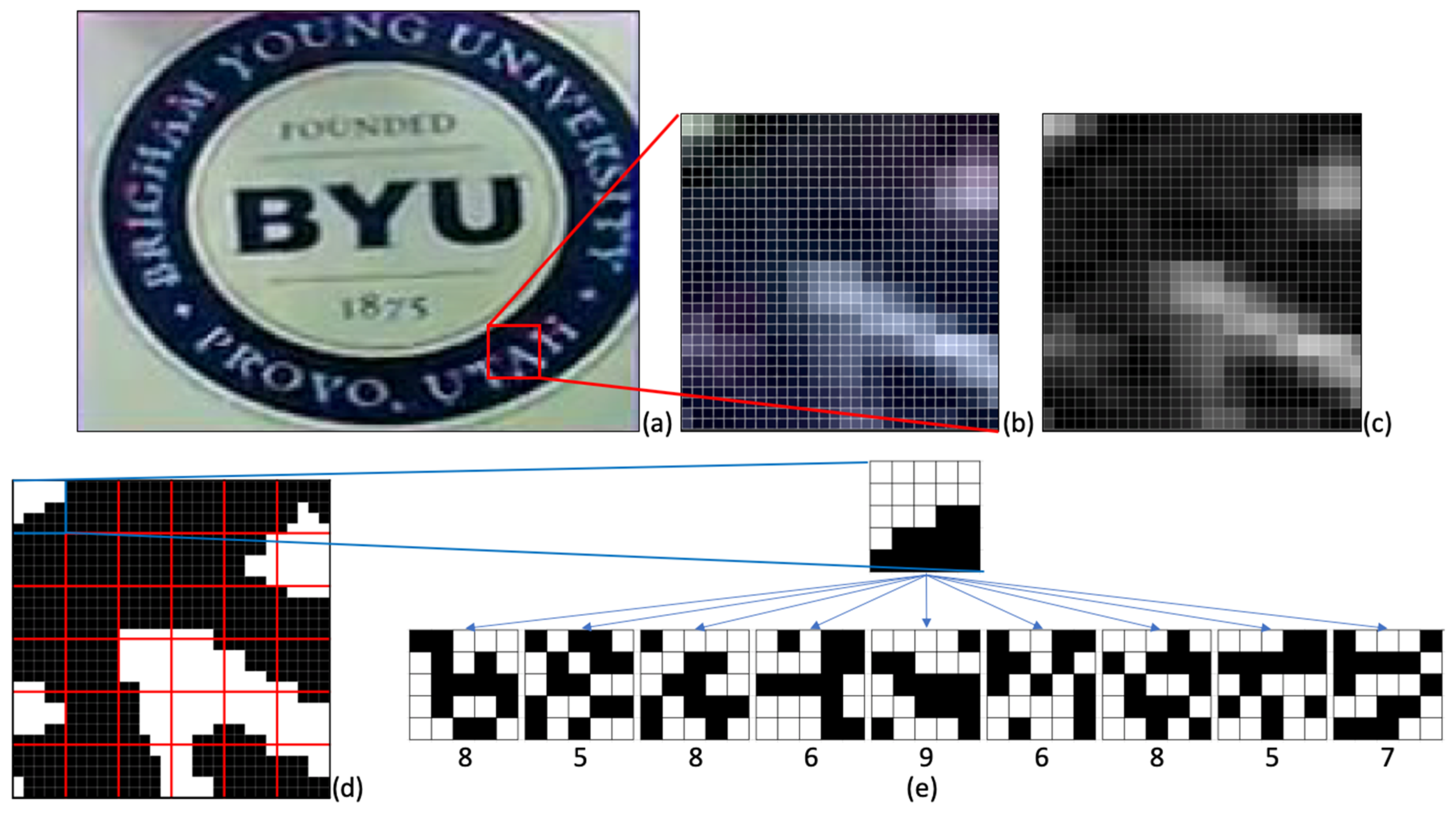
SYnthetic BAsis (SYBA) descriptor uses synthetic basis images overlaid onto a feature region to generate binary numbers that uniquely describe the feature region [8]. To efficiently detect the location of the features, SYBA can be used in conjunction with feature detection algorithms such as SIFT, or SURF to improve the process. SYBA’s descriptor of a feature region is simplified, resulting in reduced space needed to describe the feature region of interest (FRI) and time needed for comparison. Despite complexity benefits, matching accuracy of SYBA suffers due to large variations in rotation, and scaling of the feature region in the second image. If the feature is rotated or scaled differently, the pixels contained in the FRI of the subsequent image would be different or located at a different point in the FRI. This results in a significantly different descriptor value between two images which produces poor matching results. Using affine feature points as shown in [26], points likely to deform in subsequent images can be removed, however this comes at the cost of potential matches and reduces the percentage of features matched.

This paper proposes new methods that make SYBA rotation and scale invariant. Rotation invariance is achieved by manipulating the FRI in each image such that the rotation of the FRI is normalized. Scale invariance is achieved by scaling the FRI to different scales and comparing the FRI of the first image to the different scaled versions of the next. Using these methods, SYBA’s matching accuracy and total number of matches is greatly improved.

3. Algorithm

Inspired by the recent development of compressed sensing theory [27], we develop Synthetic Basis Feature (SYBA) descriptor to uniquely describe the FRI [8]. SYBA is designed to be efficient and hardware friendly [8,28]. It is shown that SYBA generates accurate matches under small amounts of image variation between frames. However, these results suffer under large amount of image rotation and scaling variation. We develop a new version of SYBA and call it robust Synthetic Basis Feature Descriptor (rSYBA). rSYBA was first introduced in [29]. It provides a compensation to scaling and rotation of FRI by normalizing the FRI during a pre-process step to improve the robustness of the feature descriptor in terms of scale and rotation invariances.

3.1. SYBA Feature Descriptor

Figure 1 illustrates the flow of SYBA algorithm. Figure 1a shows an example input image. Feature points must be detected before description and matching can be performed. In general, any feature detectors could be used to detect features. In this work, SURF is selected for feature detection because of its performance and popularity, as well as the convenience and fairness for comparisons [8].

There are two parameters that could impact the performance and the size of the SYBA descriptor. One is the FRI size and the other one is the SYBA descriptor size. The 30 × 30 FRI size is selected according to our previous result reported in [16]. Smaller FRI’s could lose important feature information. Larger FRI’s could include the background or non-feature information that affects the performance. For the SYBA size, the bigger the SYBA size, the larger and more SBI’s are needed, which increase the number of operations and descriptor size exponentially. A compromise is to divide the 30 × 30 FRI into 36 5 × 5 subregions and use 36 SYBA 5 × 5 to describe the 30 × 30 FRI.

Once a feature point is detected, a 30 × 30 region surrounding the feature point (highlighted in red in Figure 1a) is extracted and used as the FRI to represent the feature point. Figure 1b shows the detail of the pixels in the FRI. Its grayscale version is shown in Figure 1c. The FRI is binarized using the average intensity of the 30 × 30 FRI as the threshold. The binary FRI is shown in Figure 1d with the pixels brighter than the threshold set to 255 and pixels darker than the threshold set to 0. The binarization provides simple quantization of the FRI while maintaining the spatial and structure information. It also provides a certain degree of illumination invariance.

The SYBA algorithm divides the 30 × 30 FRI into 36 5 × 5 subregions [8]. According to the compressed sensing theory [27], a 5 × 5 subregion can be uniquely described by a series of 5 × 5 binary synthetic basis images (SBIs) [27]. With half of the SBI pixels (25/2 = 13) randomly set to 255, it takes nine of these 5 × 5 SBI’s to describe a 5 × 5 region. As shown in Figure 1e, every 5 × 5 subregion is compared to each 5 × 5 binary synthetic basis images to obtain a similarity measure by counting how many pixels with a value ‘255’ in a 5 × 5 subregion of the BFRI also have a value ‘255’ at the corresponding pixel in the SBI.

Figure 1 illustrates how the similarity is measured. Between the 5 × 5 subregion of the binary FRI shown on the top and the first SBI (on the left), eight pairs of corresponding pixels are both 255. Comparing the 5 × 5 subregion to the second SBI from the left, five pairs of pixels are both 255. Using this similarity measure, the 5 × 5 subregion is described by a sequence of nine numbers (8, 5, 8, 6, 9, 6, 8, 5, 7) between 0 and 13 (due to maximum 13 pixels are 255 in every SBI). With 36 5 × 5 subregions and nine numbers to describe each of them, the feature descriptor for each FRI requires 36 × 9 × 4 = 1296 bits, with four bits being needed to store a number between 0 and 13.

As mentioned previously, our aim is to develop a hardware friendly algorithm for Field Programmable Gate Arrays (FPGAs) implementation. Many embedded vision applications require the vision sensor to be low power consumption and compact in size. FPGA is an excellent option for these applications. Different computing platforms have varying computational power, which makes it difficult to compare the processing speed sand resource usage objectively. We use the number of operations to compare the processing speed and the descriptor size to compare the resource usage instead [8]. We reported the comparisons between SYBA and other well-known algorithms such as SIFT, SURF, BRIEF, and rBRIEF to prove the suitability of SYBA for hardware implementation and for real-time embedded applications.

Using the SYBA descriptor, two feature points can be matched by calculating the distance between the two descriptors. We use the L1 norm rather than other common comparison metrics such as Euclidean or Mahalanobis distance, which require complex operations such as multiplication and square root, to minimize the computational complexity. The equation for the L1 norm to compute the distance is as follows:

$$d={{\displaystyle \sum }}_{i=1}^n\left|x_i-y_i\right|,$$

(1)

where x_i and y_i represent the similarity measure (the unsigned value) for all n comparisons where n is the total number of SBIs times the number of subregions. A distance close to zero indicates a perfect match and a large distance represents a poor match.

3.2. Robust SYBA Feature Descriptor

Although SYBA descriptor is smaller and more efficient than other methods while maintains high matching accuracy, its performance suffers when large rotation and scaling variations exist between two images. For example, if the image is rotated because of camera movement, the FRI could also rotate slightly. Although the FRI rotation is not as obvious as the whole image, the feature descriptor could still change, resulting in high L1 norms. To cope with this challenge for certain applications, the descriptor calculation must account for rotation and scaling variations. rSYBA is developed to perform a pre-process step such that the region used as FRI is scaled and rotated to generate a few extra FRI’s for description and matching [29].

3.2.1. Scale Invariance

To achieve scale invariance, rSYBA re-scales the FRI to different scales while maintaining the same dimensions and location within the image. This results in multiple FRIs and hence multiple feature descriptors corresponding to one feature point. Feature matching is achieved by matching either the feature from the first image to the best scaled feature in the second image or vice versa. Figure 2 illustrates how scaling invariance is achieved. The original FRI from the first image on the left is highlighted in red. This FRI is scaled to 0.9, 1.0, and 1.1. Feature descriptors for these three scaled FRIs are matched against the feature in the second image. In this example, the best match is determined to be the one scaled to 1.1.

The number of scales is dependent on the application and camera frame rate or camera movement. Most modern cameras operate at 60–120 frames per second, the scale difference that may occur between two consecutive frames can be small if the camera does not move at high speed. The scale factors from 8 to 1.2 with 1 scaling intervals should be adequate for most applications. These scale factors generate 5 FRIs for one detected FRI. Only three of them are shown in Figure 2.

3.2.2. Rotation Invariance

SIFT and SURF both calculate the dominant gradient orientation of the feature region and normalize the descriptor value by subtracting that dominant orientation from the descriptor to make the description rotation invariant. Instead of normalizing the resulting descriptor, rSYBA normalizes the FRI directly by rotating the FRI by the dominant gradient orientation. The gradient value and orientation at each pixel location are computed using Equations (2) and (3).

$$m\left(x,y\right)=\sqrt{{(I\left(x+1,y\right)-I\left(x-1,y\right))}^2+{(I\left(x,y+1\right)-I\left(x,y-1\right))}^2}$$

(2)

$$\theta \left(x,y\right)=ta{n}^{-1}\frac{I\left(x,y+1\right)-I\left(x,y-1\right)}{I\left(x+1,y\right)-I\left(x-1,y\right)}$$

(3)

where m represents the gradient magnitude and θ represents the gradient orientation. I represents the grayscale pixel value at the specified x and y locations within an image. For hardware implementation, instead of using the costly multiplication, square root, and tangent operations, a Gaussian kernel can be applied to the image to find the gradient magnitude and orientation.

Using these gradient orientations and magnitudes, a histogram is generated with each bin corresponding to a range of gradient orientations. The range for the bins is dependent on the application. As mentioned previously, with high camera frame rate, rotation from frame to frame is small and it is even smaller for the FRI. Figure 3 shows an example histogram with a range of 10 degrees.

The gradient and orientation are computed for each pixel value contained in the FRI. The corresponding gradient orientation bin in the histogram is incremented by an amount proportional to the gradient magnitude. The resulting histogram represents the total gradient magnitude for each gradient orientation bin. The gradient orientation of the bin that has the highest gradient magnitude is selected as the dominant gradient orientation. A sample of this histogram is shown in Figure 3. The total gradient magnitude is normalized to 100% for display.

Using this orientation, the FRI is back-rotated by the dominant gradient orientation. Equations for rotation transformations of an image are shown as Equations (4) and (5).

$$x_2=\cos \theta \cdot \left(x_1-x_0\right)-\sin \theta \cdot \left(y_1-y_0\right)+x_0$$

(4)

$$y_2=\sin \theta \cdot \left(x_1-x_0\right)+\cos \theta \cdot \left(y_1-y_0\right)+y_0$$

(5)

where x₂ and y₂ correspond to the re-mapped coordinates of the pixel and θ corresponds to the rotation angle. The center coordinates of the rotation region are x₀ and y₀, while x₁ and y₁ correspond to the pixel being mapped. For hardware implementation, the multiplication of a cosine or sine of an image location can be performed with a look-up table. The size of the image is bounded (most images are less than 2000 pixels in one dimension) and the angle degrees for the dominant orientation are fixed at an internal of 10 degrees, thus a maximum of 36 possible angle values can be found. For an 8-bit memory cell, the sine and cosine look-up tables can be represented with, at most, 36 × 2000 = 72 KB of memory. Surrounding pixels are included around the FRI such that when the region is rotated no information is lost. The region is also cropped such that the rotated image fits within the FRI dimensions.

Rotation invariance is achieved through this method as the matching FRIs are rotated to approximately their normalized orientation. Additional rotated FRIs are generated if there is an orientation found that is within the 80% range of the max magnitude using the histogram. This percentage threshold can be adjusted based on the application to reduce the number of generated rotated FRIs. If the application has a large amount of rotation between frames, a lower percentage is recommended. This is done to account for any sort of noise or distortions that would shift the dominant gradient values but at the price of more rotated FRIs for description and matching.

Figure 4 illustrates the rotation invariance operation. Once a feature is detected and its FRI is defined (small blue square), the FRI is expanded (dotted blue square) for rotation. As shown in the gradient orientation histogram in Figure 3, there are two dominant orientations. One has the maximum accumulated gradient magnitude at 20 degrees. The second one has the accumulated gradient magnitude larger than the 80% threshold at 300 degrees. The extended FRI is rotated for 20 and 300 degrees to generate two rotated FRIs for description and matching.

Unlike scaling invariance that only FRIs from one image must be scaled to generate multiple scaled FRIs for matching, rotation invariance requires feature regions from both images to go through the same process to normalize orientation. Normally, only one rotated FRI is needed per feature point unless more than one dominant gradient orientation exists as shown in Figure 3.

4. Experiments

Feature detection is the first step of feature matching. As the start of the algorithm, feature detection is exerted on the input image frame to find feature points. In general, any feature detection algorithms could be employed. In this work, SURF is selected to detect feature points for its performance and popularity, as well as the convenience and fairness for comparison [8].

Two datasets were used to compare the algorithm performance to prove that rSYBA results in improvement under large amounts of rotation and scaling image variation. The first dataset is the BYU Scaling and Rotation dataset. This dataset consists of images that are scaled to 0.8, 0.9, 1.1, and 1.2 and images that are rotated by 5, 7, 10, and 15 degrees. The scaling factors and rotation angles are known in this dataset. We use this dataset to demonstrate that rSYBA has superior scaling and rotation invariance than the original SYBA. The second dataset is the Oxford Affine dataset [26]. The Oxford Affine dataset consists of image sequences that were designed to test the robustness of feature descriptor algorithms with image perturbations such as blurring, lighting variation, viewpoint change, zoom and rotation, and image compression. Since this work focuses primarily on rotation and scaling, the “Boat” sequence of zoomed and rotated images was used for comparing rSYBA with the other algorithms.

4.1. Comparison Metrics

To quantify the merit of one algorithm versus another, common metrics such as precision and recall are used. Precision and recall are computed as Equations (6) and (7).

$$precision=\frac{\#\mathrm{Correct}\mathrm{Feature}\mathrm{Matches}}{\#\mathrm{Matches}\mathrm{Found}}$$

(6)

$$precision=\frac{\#\mathrm{Correct}\mathrm{Feature}\mathrm{Matches}}{\#\mathrm{Matches}\mathrm{Found}}$$

(7)

Using these metrics, we can plot a precision vs. recall curve to get an approximation of how accurate the feature matches are as well as the efficiency of the algorithm in producing correct feature matches. Because the total number of possible matches (the denominator of recall in Equation (7)) is unknown or subjective but remains constant for each image, it is equivalent to use the total number of correct matches as recall for our comparisons. We also compute the accuracy as the percentage of the matches found that there are correct matches. It is similar to calculating the precision when the maximum number of correct matches is found.

To determine the correctness of the final matched feature pairs between two images, the homography matrix was used [8]. We used the matched pairs to find the homography matrix, which transforms the image points in one image to their corresponding locations in the second image. Equation (8) shows this,

$$p_2=H\cdot p_1$$

(8)

where H is the homography matrix, p₁ is the point in the first image, and p₂ is the point in the second image. Outliers and incorrect matches are filtered out in the computation of the homography matrix using the RANSAC algorithm [30]. This homography calculation is not necessary for benchmark datasets that often provide a ground truth homography. To determine if a match is correct, the matched feature point must be within a certain range of the mapped feature point. For these experiments, the error bound was set to five pixels.

4.2. BYU Scaling and Rotation Dataset

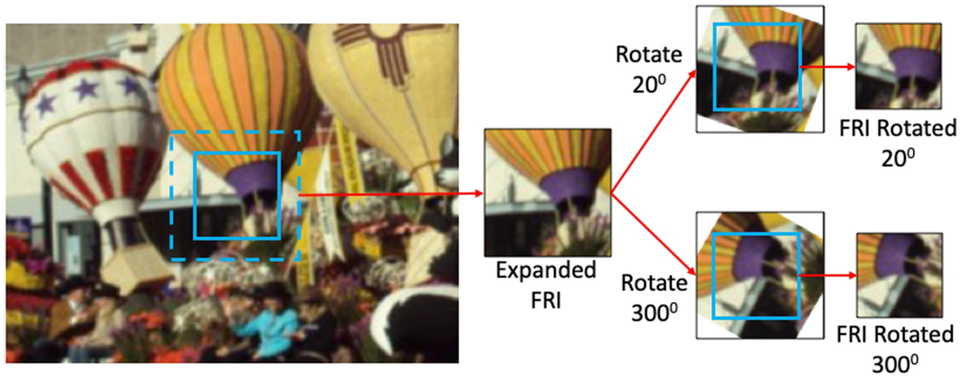
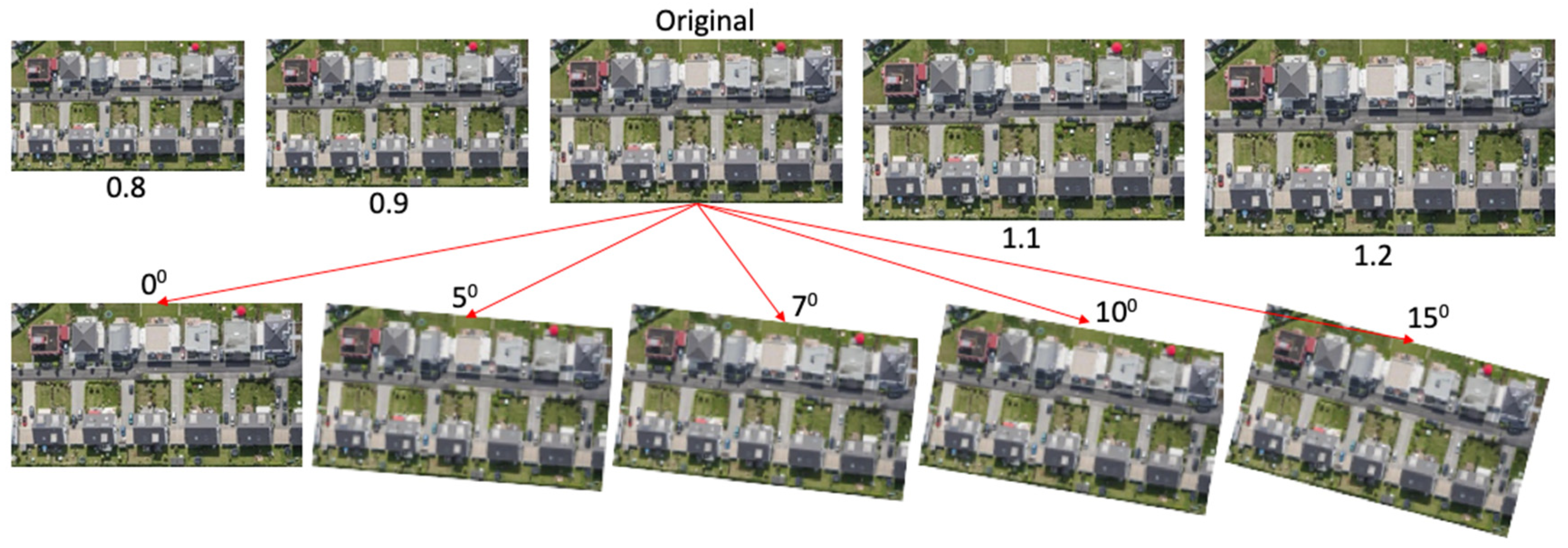
This experiment focuses on demonstrating the improvements we made for rSYBA provide better scaling and rotation invariance than the original SYBA. We created a small dataset called BYU Rotation and Scaling Dataset for this experiment. It starts with one aerial image. This original image is then scaled to 0.8, 0.9, 1.1, and 1.2. It is then rotated by 5, 7, 10, and 15 degrees. The size of the original image is maintained the same for the rotation set. All these images in the dataset are shown in Figure 5.

In our experiments, features detected at the edge of the image were filtered as they are the most likely to be incorrect matches due to kernel filtering. Features were then matched using SYBA and rSYBA. Feature matches were ranked based on the L1 norm distance as well as the distance to the next best match. The smaller the L1 norm distance and the larger the distance to the second-best match resulted in a larger confidence of being a good match.

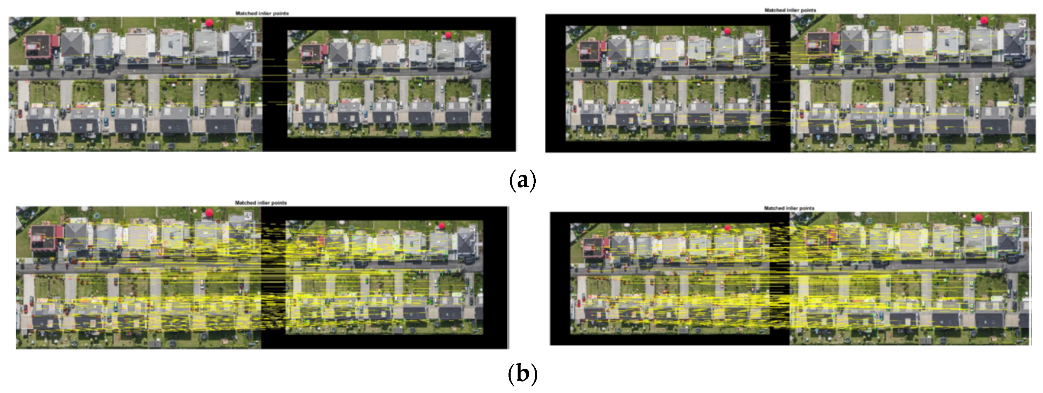
We matched features detected from the original image to the features in the scaled and rotated images to compute the matching accuracy as explained in Section 4.1. We also computed precision vs. recall in terms of the number of correct matches for comparison. Visual results for scaling sequence are shown in Figure 6a SYBA and Figure 6b rSYBA, where the yellow lines connect the correct matches.

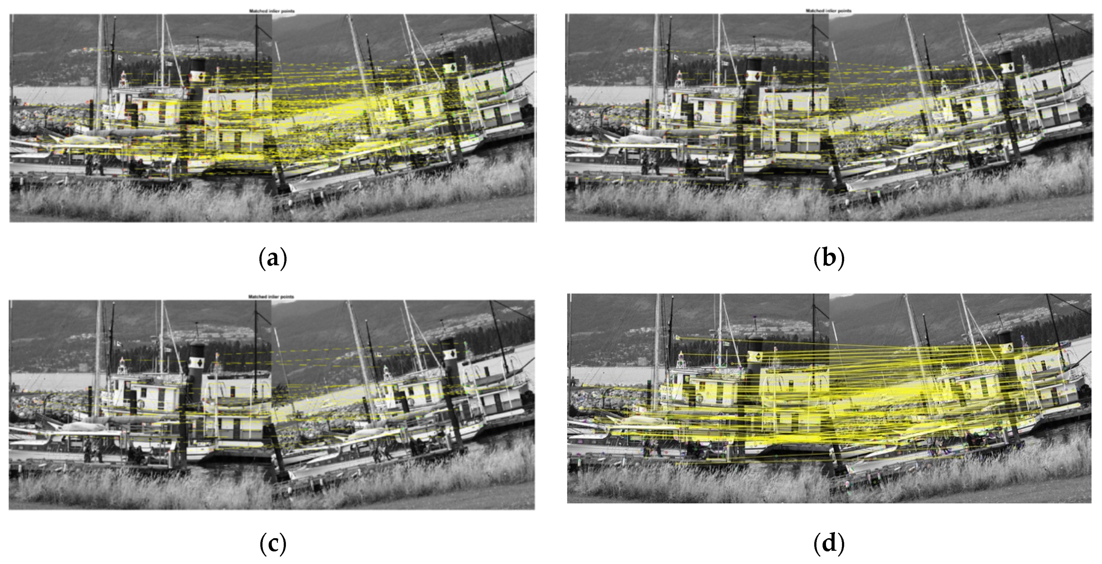
The results for the rotation sequence also demonstrated a significant improvement from SYBA to rSYBA. Visual results are shown in Figure 7a SYBA and Figure 7b rSYBA.

Table 1. Accuracy comparison for Scale Image Sequence.

Scale Factor	Feature Count	# of Matches Found		# of Correct Matches		Accuracy (%)		Recall (%)
		SYBA	rSYBA	SYBA	rSYBA	SYBA	rSYBA	SYBA	rSYBA
0.8	300	30	185	8	166	26.66	89.72	2.67	55.33
0.9	300	67	222	44	211	65.67	95.04	14.67	70.33
1.05	300	111	249	101	237	90.99	95.18	33.67	79.00
1.1	300	81	234	61	221	75.30	94.44	20.33	73.67
1.2	300	44	217	21	201	47.72	92.62	7.00	67.00

and

Table 2. Accuracy comparison for Rotation Image Sequence.

Degrees	Feature Count	# of Matches Found		# of Correct Matches		Accuracy (%)		Recall (%)
		SYBA	rSYBA	SYBA	rSYBA	SYBA	rSYBA	SYBA	rSYBA
5	300	74	203	59	190	79.72	93.59	19.67	63.33
7	300	35	160	9	139	25.71	86.88	3.00	46.33
10	300	33	175	18	162	54.54	92.57	6.00	54.00
15	300	20	150	9	137	45	91.33	3.02	45.67

show all the computed metrics for SYBA and rSYBA for each image comparison in each sequence. We compute the accuracy as the percentage of the matches found that are correct matches when the maximum number of correct matches is found. As explained in Section 4.1, the feature count is the denominator and can be cancelled out when plotting the precision vs. recall curve. We set the feature count to 300 to calculate the recall because the maximum features found are all below 300.

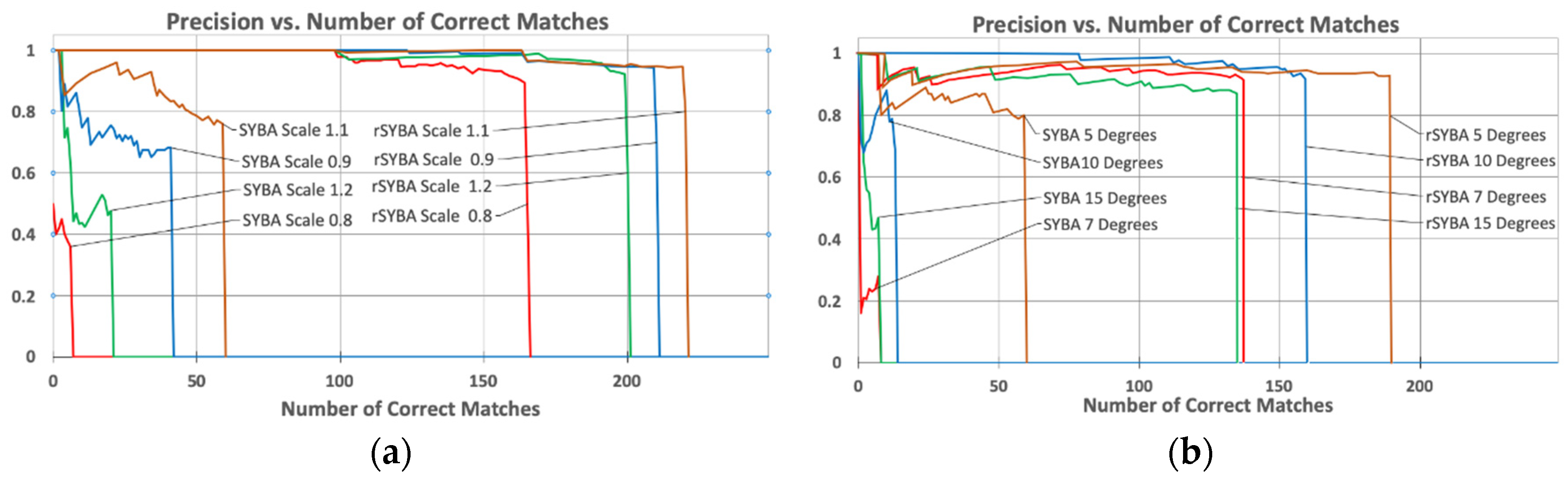
We included a scale of 1.05 to test the accuracy when there is a very small variation. As shown in the tables, rSYBA provides a significant increase in number of matches and number of correct matches compared to SYBA. On average across the test cases for the scaling dataset, rSYBA improved recall percentage by 53.578% and accuracy by 32.132%. On average across the test cases for the rotation dataset, rSYBA improved recall percentage by 44.55% and accuracy by 39.85%.

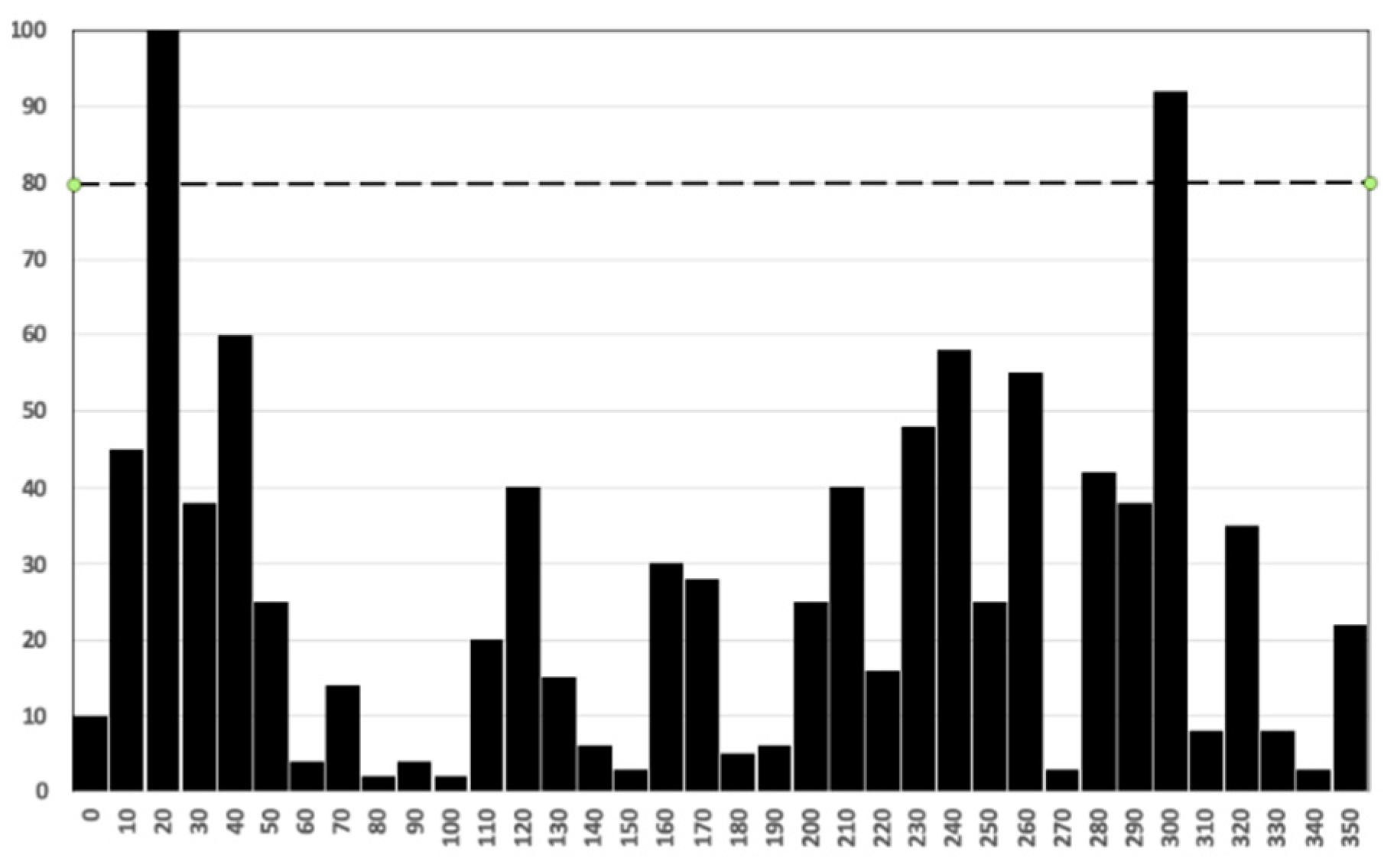
Overall precision of rSYBA and SYBA was also compared. We performed matching precision comparison by adjusting the matching parameters to generate different numbers of correct matches and computing their corresponding precision. As explained in Section 4.1, we use the number of correct matches to represent the recall percentage. For this comparison, these precision metrics were calculated for each algorithm applied to each image with differing amounts of image variation. Results of this investigation, as well as a visual comparison of the final total number of correct matches, for each sequence are shown in Figure 8a for scaling and Figure 8b for rotation variations.

Data analysis results support that rSYBA will consistently outperform SYBA even if the algorithms are forced to match all possible features (irrespective of matching thresholds). The dips at the beginning of the graph are due to an incorrect match detected early in the data acquisition when the total number match count is low. Despite these dips, the trends will smooth and integrate out over time as the match count increases. These graphs show the trend until the matching algorithm can no longer produce any more matches, which is represented by the sudden drop of precision to 0.

4.3. Oxford Affine Dataset

Extensive comparisons between SYBA and other mainstream methods have been performed and reported in [8] to show SYBA’s superior performance. In this work, we focus only on the improvement of rSYBA over SYBA. We include comparisons between rSYBA and representative intensity (SURF), binary (BRISK), and the new ORB descriptors. SURF is the most widely used feature detection algorithm and contains aspects which account for rotation and scaling variance between images. BRISK is a commonly used compressed feature description algorithm. ORB is the improved version of BRIEF that is designed to provide robust rotation invariance.

Oxford Affine Features dataset was used for this experiment [26]. It contains sets of 6 images, with increasing variation in each consecutive image. For example, Image 1 in each set of images represents the original image. Images 2–6 are images with increasing image deformation. We used the “boat” dataset in the Oxford dataset which contains images with zoom and rotation variance. We used the same methods discussed in Section 4.1 for comparison. rSYBA’s overall performance was compared with SURF, BRISK, and ORB using Image 1 versus Image 2 and Image 1 versus Image 3 of the dataset in Matlab. We did not compare with more images contained in the dataset because no algorithm produced enough matches to give sufficient data for a meaningful comparison.

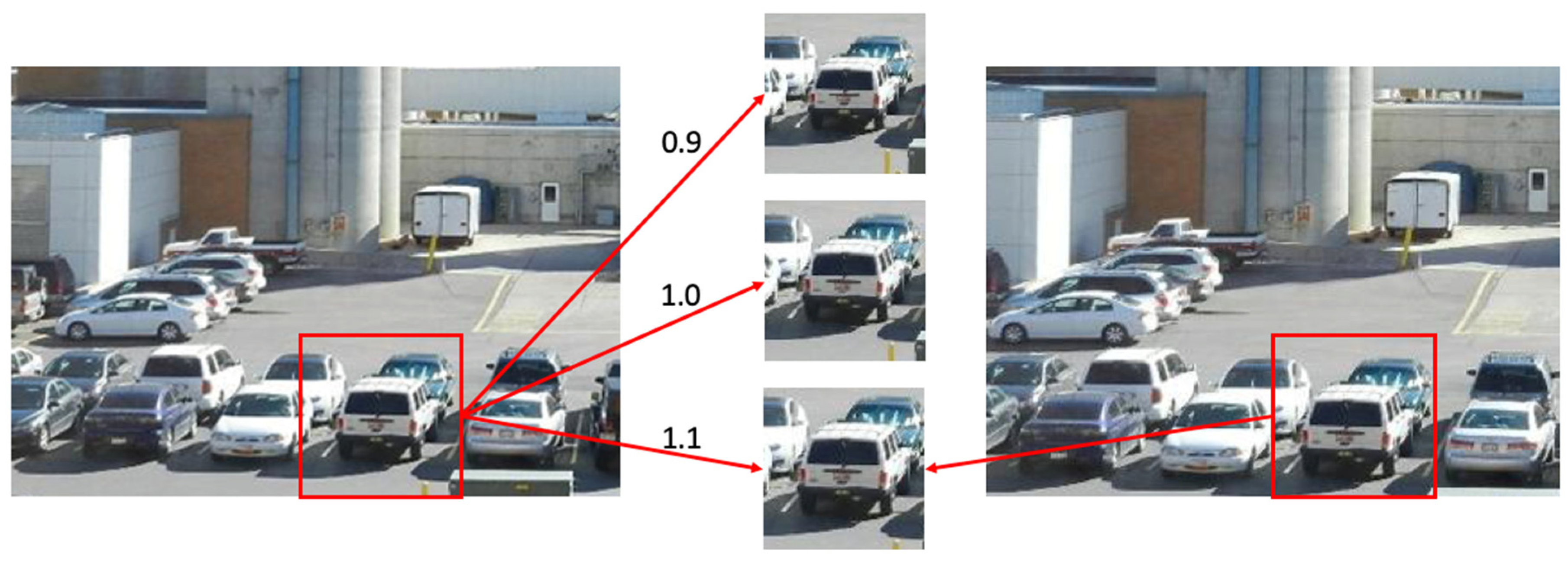
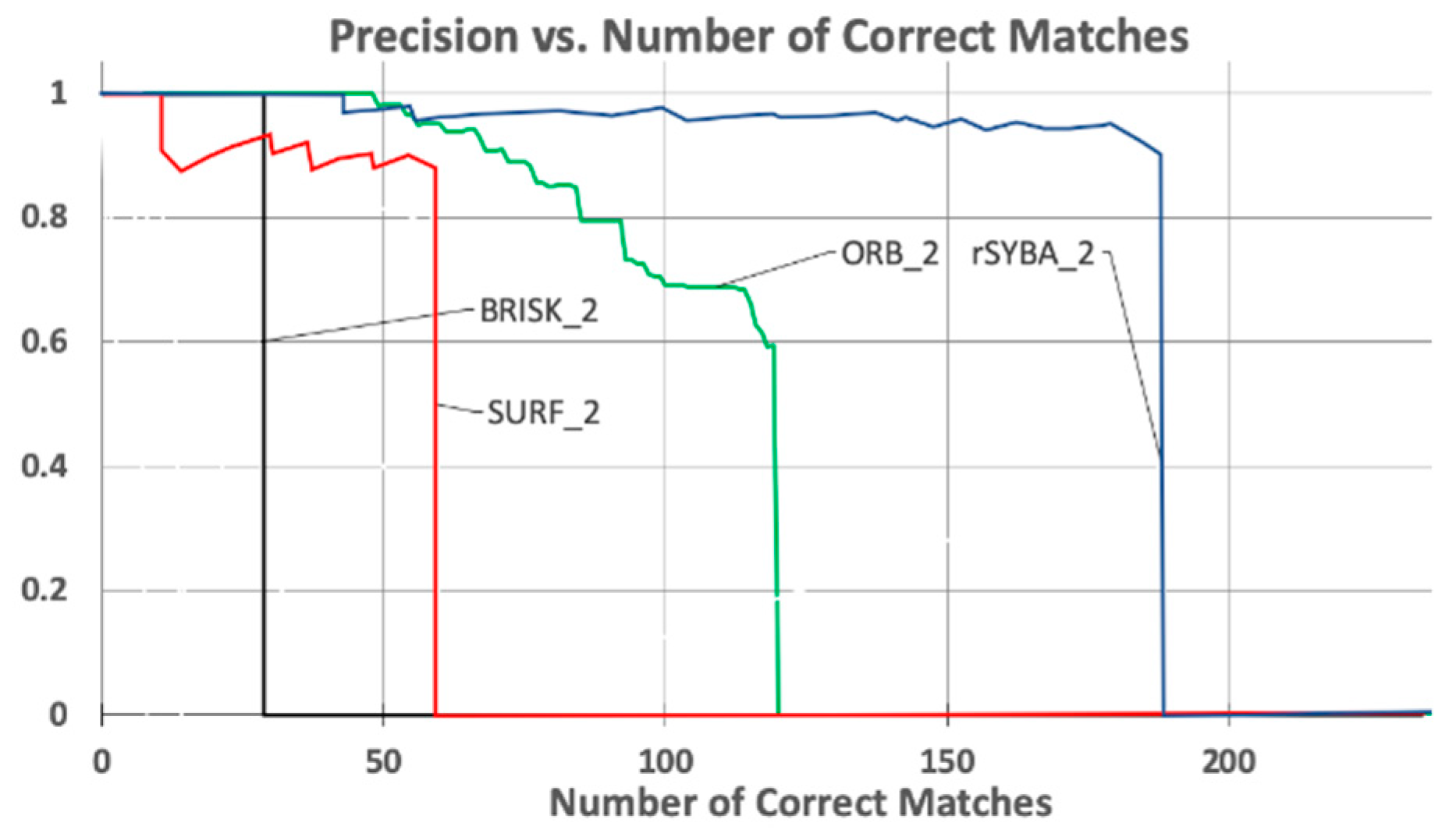
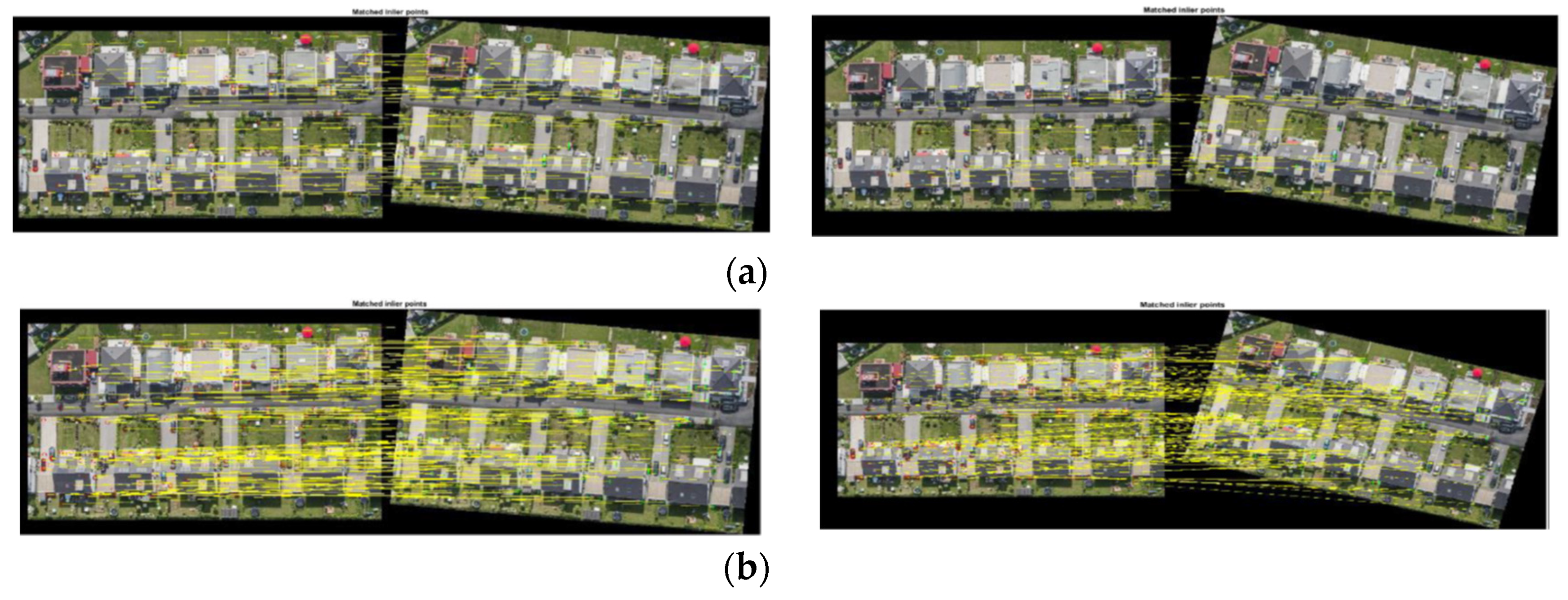
Figure 9 shows the matching results between Images 1 and 2 in the Oxford boat sequence with rSYBA, SURF, BRISK, and ORB respectively.

Table 3. Metrics Boat Image Sequence between Images 1 and 2 and Images 1 and 3.

Image Pair	Feature Count	# of Matches Found				# of Correct Matches				Accuracy (%)				Recall (%)
		rSYBA	SURF	BRISK	ORB	rSYBA	SURF	BRISK	ORB	rSYBA	SURF	BRISK	ORB	rSYBA	SURF	BRISK	ORB
1 & 2	500	197	70	30	200	190	62	30	119	96.44	88.57	100.00	59.50	38.00	12.40	6.00	23.80
1 & 3	500	171	13	0	170	139	2	0	41	81.28	15.38	0.00	24.12	27.8	0.40	0.00	8.20

shows the metrics for the output of each of these algorithms. Precision vs. recall curve is shown in Figure 10.

Overall, although with higher accuracy between 1 and 2, BRISK produced very few matches and very few correct matches for real-world applications. For image pair 1 and 2, ORB produced 3 more matches than rSYBA (200 vs. 197) but only 119 of its 200 matches were considered correct matches (within five pixels of the mapped features from homography) as opposed to rSYBA’s 190 of 197. In comparison, rSYBA produced a significant higher number of correct matches and maintained a high accuracy as compared to SURF, BRISK, and ORB. This demonstrates that rSYBA can improve results as compared with mainstream algorithms in applications that contain a large amount of image variation.

We calculated the recall using Equation (7). As explained in Section 4.1, the number of possible matches is unknown or subjective, we picked the number of possible matches to be large enough to include all correct matches. In this case, the number of possible of matches was set to 500. Recalls shown in Table 3 are the correct matches divided by 500. We plot the precision vs. recall curve in Figure 10. Instead of using Equation (7) to calculate recalls for this plot, we plot the curve using the number of correct matches (the numerator of Equation (7)) because the denominator (500) can be cancelled.

5. Applications of rSYBA

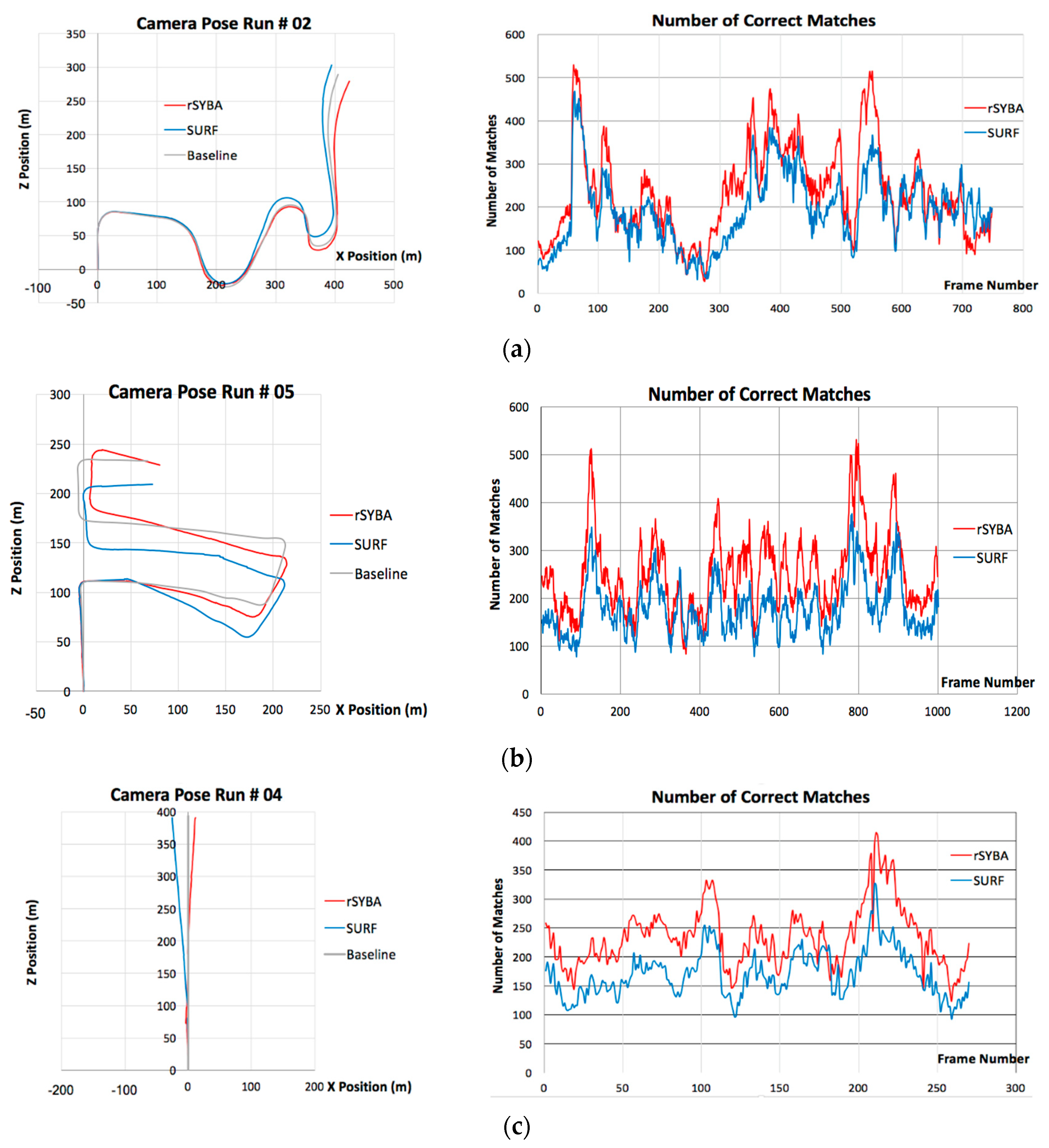
This paper exerts rSYBA in two applications that utilize high amounts of image variation to demonstrate its improvements over the original SYBA. The first shows camera pose plotting for a ground-based vehicle using monocular visual odometry. The second consists of generating panoramic images through image stitching and image transforms. Both applications contain large amounts of image variation between image frames and therefore requires a significant amount of correct feature matches to generate acceptable results. As shown in Table 3, although ORB produces more matched features and correct matches, SURF has the best accuracy among the three representative algorithms we compared. In this section, we only include results from SURF for comparison.

5.1. Visual Odometry

In this subsection, we describe an application of a Monocular Visual Odometry (VO) to detect the 3D camera positioning with a ground vehicle. We used the rSYBA feature descriptor algorithm to obtain accurate feature matches to be used in the VO application. Additionally, we compared our 3D camera positioning results using rSYBA with results taken using SURF. Results were taken using the industry standard VO dataset called KITTI [31].

To start the VO algorithm, feature points are extracted from the current image frame (I_k) and the previous image frame (I_k−1). Feature matching is then performed using the rSYBA descriptor algorithm between frame I_k−1 and I_k. The essential matrix between these two frames is computed using feature correspondences and then decomposed into rotation (R_k) and translation matrices (t_k) which can be used to extract 3D positioning information [32]. Feature point positioning is then updated using the techniques discussed in [28] to reduce drift and error between frames. Camera motion between time k−1 and k is rearranged in the form of the rigid body transformation $P_k\in R^{4\times 4}$:

$$P_k = \left[\begin{array}{cc}{R}_k& t_k\\ 0& 1\end{array}\right]$$

(9)

where $R_k\in R^{3\times 3}$ the rotation matrix, and $t_k\in R^{3\times 3}$ the translation vector. The set P contains the camera motion in all subsequent frames. Using the rotation and translation vectors, we have the 3D transformation matrices necessary to transform the camera pose in the previous frame to find the camera pose in the current frame. The current camera pose can be computed by concatenating all the transforms for each frame up to and including the transform for the current frame.

The proposed method was evaluated by using publicly available real-world datasets from the KITTI benchmark suite [31]. The KITTI dataset contains images for stereo VO, but for this application we used a single camera video sequence or monocular VO.

For performance evaluation of this application, the relative error in distance and the root mean square error (RMSE) were found and used as comparison metrics between rSYBA and SURF. The relative error in distance is calculated as shown in Equation (10).

$$relative error=\frac{ABS\left(ground truth length-visual odometry path length\right)}{visual odometry path length}$$

(10)

This measures the difference between the calculated length of VO path and the actual distance traveled. RMSE is calculated based on each position transformation matrix (P_k). The RMSE matrix indicates the sample standard deviation of the transformation difference between the ground truth and the visual odometry result. RMSE provides a very good measurement of the average error of the entire image sequence to determine the algorithm’s frame-to-frame performance.

The RED alone is not able to evaluate the performance very well because it only evaluates the accuracy of the distance traveled. The relative error could end up very small (measured distance is close to the actual distance travel) but along a completely different path. The RMSE measures the individual frame-to-frame accuracy and provides a better evaluation of overall performance. The RMSE computed and shown in the experimental results is the average across all the images in the sequence. For comparing feature matching accuracy, the same VO algorithm and feature detection methods were used to produce as accurate a comparison as possible between rSYBA and SURF.

In the experiment, country, urban, and country and urban mixed sequences were used for comparisons. All these sequences were recorded at different times of the day and a variety of locations which include different lighting conditions, shadow presence, numbers of cars, pedestrians, cyclists, etc. as well as paved winding roads with high slopes. Results for each case for the camera positioning plotting and the number of correct matched feature pairs are shown in Figure 11 For the camera position plotting, the X and Z dimensions of the plots are shown as these are the most significant when plotting for an autonomous vehicle (height of the ground is not really incorporated in ground vehicle navigation). The Y dimension is still included in error computations to help assess the accuracy of the feature matching algorithms with VO. It is shown that rSYBA produced more inlier matches than SURF on most of the frames in the sequence.

The overall results for the RMSE between each frame the relative error in distance for each case can be seen in

Table 4. The overall results for the RMSE between each frame the relative error in distance.

		RMSE			Relative Error Distance (%)
		X Position	Y Position	Z Position
Urban and Country	SURF	5.2252	2.204	9.6456	0.000701
	rSYBA	5.5019	2.8999	5.3489	0.000503
Urban	SURF	8.4752	13.695	25.22	0.00457
	rSYBA	7.815	6.8648	9.6699	0.00538
Country	SURF	11.914	2.6242	1.7323	0.00329
	rSYBA	4.2694	0.32006	1.7092	0.005206

. It is apparent from these results that rSYBA outperformed SURF in each sequence. For example, in the case of urban sequence, rSYBA reduced RMSE error compared to SURF in the X, Y, and Z dimension by 0.6602, 6.8302, and 15.5501 m respectively.

Figure 11 and Table 4 show rSYBA produces a more substantial number of accurate feature matches than SURF in every test case. This assists in generating a more accurate essential matrix which correspondingly shows a smaller error. Compared to SURF, rSYBA is also more suited to be implemented in hardware for embedded applications.

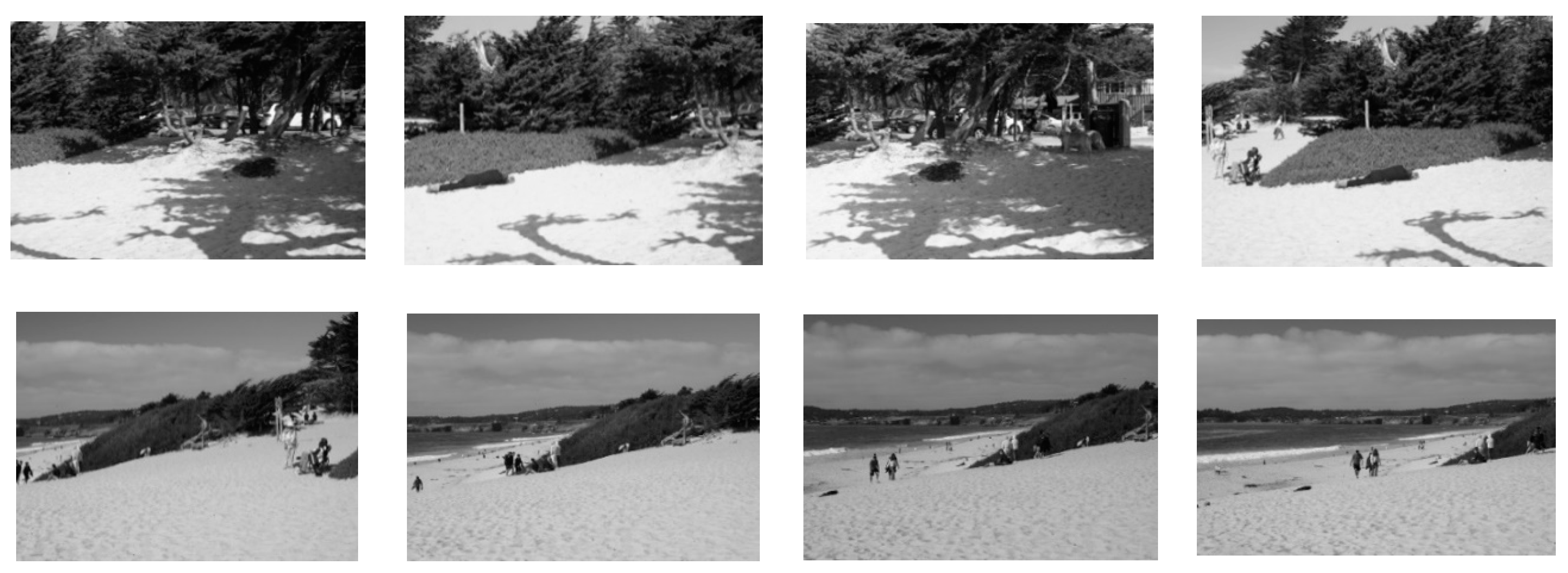
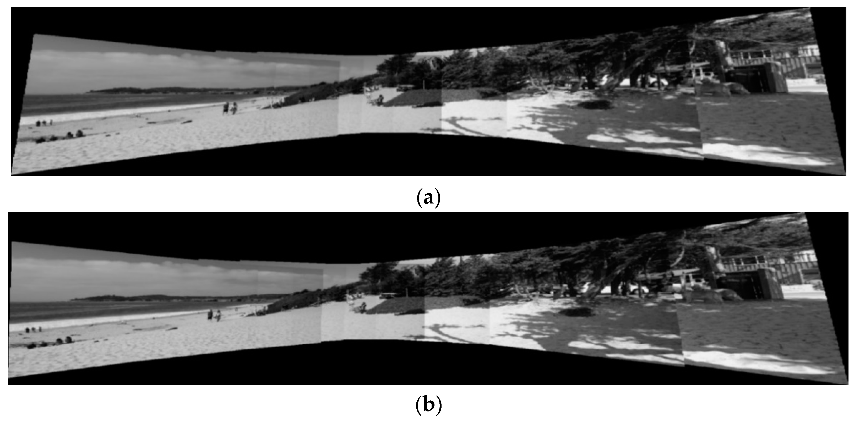
5.2. Image Stitching

For image stitching to be successful, correlation must be found between the images taken which can then be used to transform each image and overlap them to form the panoramic image. In this subsection, we present results with applying the feature-based image stitching approach with rSYBA and forego any blending technique as we are focused on the image transform results. Results were taken using the Adobe Panorama dataset, which contains 10 image sets with image transform ground truths [33]. Again, results were only compared against SURF because its high accuracy and a reasonable number of correct matches.

To start image stitching, the homographic image transform is found between each adjacent image in the panorama. The homography transform matrix is computed by using the correctly matched features between the overlapping regions in the images. After the homographies are found between each subsequent image, a new homography is computed for each image. The algorithm iterates through each homography matrix and computes the new homography transform. To normalize the panorama and center the view on the middle image in the set, the homographies are multiplied by the inversion of the center images’ computed homography. Then, the extreme transformed points are found contained within the homography transforms to find the bounds of the panoramic view. After the bounds for the new image are found, a blank image or canvas is created and masking is then used to insert all the transformed images into the panorama.

For this research, the Adobe image dataset was used for experimentation [33]. Eight images were used for each view sequence, resulting in seven homographies computed. Included in the dataset are the ground truths for the homography matrices. For the comparison metrics, the average relative error was computed for each of the values within the $3\times 3$ homography matrix across all the images in the panorama. The relative error is computed as follows:

$$relative error=\frac{ABS\left(ground truth value-computed homography value\right)}{ground truth value}$$

(11)

Results for each of the panoramic views were taken using rSYBA and SURF. Feature locations were detected using the SURF feature detection algorithm and were kept constant with all algorithms to allow for accurate comparisons.

Figure 12 shows image sequences used for testing. The images include moving subjects, which may introduce some artifacts in the panorama as the subjects that move may not align properly. The final results of the image stitching application can be seen in Figure 13. Individual images were transformed using the resulting homographies and the camera intrinsic parameters. The results for the relative error across stitching all the frames for all the algorithms can be seen in

Table 5. Average relative error results for 3 × 3 homography matrix across all images.

rSYBA				SURF
0.07142	0.39346	0.078774	Average	0.073905	0.73357	0.08524	Average
0.15547	0.07237	0.51538	0.7121	0.15859	0.07567	0.54469	0.95745
0.10578	4.9447	0.071898		0.082791	6.7907	0.07190

. Results were computed using the ground truth homographies provided with the dataset. From these results, it is shown that rSYBA, on average, produced more accurate homographies than SURF. This resulted in a more accurate panoramic view.

6. Conclusions

This paper proposed a novel idea for the improvement of a compressed sensing feature description algorithm. rSYBA provides robustness to SYBA with a pre-processing step to compensate the transforms of scaling and rotation of FRI. rSYBA maintains the reduced storage space and complexity as the original SYBA while increasing the number of matched feature points and maintaining feature point matching precision. Experiments were performed using common comparison methods with precision and recall computations. Results show that rSYBA produces higher precision rates and number of correct matches compared to SYBA as evidenced by the BYU Rotation and Scaling dataset. rSYBA also competes favorably with mainstream algorithms as shown by the Oxford dataset. By being applied to some widely used computer vision applications, including object detection, visual odometry, and image stitching, rSYBA also shows superior performance against mainstream algorithms.