Analysis of Counting Bloom Filters Used for Count Thresholding

Abstract

A bloom filter is an extremely useful tool applicable to various fields of electronics and computers; it enables highly efficient search of extremely large data sets with no false negatives but a possibly small number of false positives. A counting bloom filter is a variant of a bloom filter that is typically used to permit deletions as well as additions of elements to a target data set. However, it is also sometimes useful to use a counting bloom filter as an approximate counting mechanism that can be used, for example, to determine when a specific web page has been referenced more than a specific number of times or when a memory address is a “hot” address. This paper derives, for the first time, highly accurate approximate false positive probabilities and optimal numbers of hash functions for counting bloom filters used in count thresholding applications. The analysis is confirmed by comparisons to existing theoretical results, which show an error, with respect to exact analysis, of less than 0.48% for typical parameter values.

1. Introduction

A bloom filter (BF) is a powerful tool that can be used to create novel, low-overhead methods for dealing with big data sets in various software/hardware applications. Proposed by Burton Howard Bloom in 1970 [1], a BF is an m-bit vector that is initialized to 0. Assuming that n elements are stored into a data set, each time a new element is stored, k hash functions, each of which maps the element to one of m bit locations, are applied and the corresponding bits in the BF are set to 1. To determine if a new unknown element is a member of the data set or not, the k hash functions are applied to that element and the corresponding bits in the BF are checked. A positive answer is returned if all of those bits are found to be 1. Since the search time is independent of the number of elements in the data set, this results in extremely space-efficient and fast search of large data sets. Although false positives are possible, false negatives are not since the element could not have been stored in the data set if any of the k hash function bits in the BF are 0.

Over the years, various BF variants have been proposed. One commonly cited variant is a counting bloom filter (CBF), which has been proposed as a method that supports deletion as well as addition of elements to a data set [2]. In a CBF, the m elements are multiple-bit counts instead of bits. Every time an element is added to or deleted from the data set, k hash functions are applied to the element and all of the k locations in the m-element CBF are incremented or decremented by one. In order to check if a specific element is still in the data set, the k hashed locations in the CBF can be checked for the absence of 0 values. Several methods have been proposed to enable efficient support of m-element CBFs [3,4].

BFs and CBFs have been found to be useful for numerous applications. For example, in a web cache, instead of storing all web objects that are accessed, disk writes can be significantly reduced by only storing those web objects that are referred to more than once, thereby eliminating “one-hit wonders” (accessed by a set of users once and never again). A BF can be used to quickly determine if a specific web page has been referenced before or not. For long-term usage, a CBF can be used instead of a BF in order to permit deletion of long unused web objects from the web cache. This approach has been found to reduce the rate of disk writes by nearly half in an actual system of servers [5].

Other applications where BFs and CBFs have been found to be useful include communications and networking applications [6,7,8,9], Huffman coding [10], cache architecture design [3,11], memory wear leveling [4], and string search for DNA sequence identification [12,13,14,15].

Given that the elements in a CBF contain approximate “counts”, this paper examines the problem of using a CBF as an approximate counting mechanism, in particular to check whether a certain data element has been referred to $\theta$ or more times, where $\theta$ is a count threshold. For example, when applied to the above web cache application, $\theta =2$ could be used to eliminate one-hit and two-hit web objects; i.e., disk write usage could be reduced by only storing web objects that have been accessed two or more times. As a second example, when applied to memory management in a computer system, a value such as $\theta =5$ could be used to identify hot memory addresses. As a third example, when applied to DNA sequence identification, approximate count thresholding could be used to quickly identify or match specific strings in a DNA sequence that occur more than $\theta$ times. As a fourth example, approximate count thresholding could be used to determine if a set of nodes are accessing a given web page a large number of times within a short timespan and thus help guard that web page against distributed denial of service (DDOS) attacks [16].

The main motivation for this paper to provide a solid theoretical foundation for the use of CBFs for count thresholding applications. Towards this end, Section 2 introduces the traditional BF and CBF analysis. Then Section 3 presents the newly proposed CBF analysis method and its main results. Next, Section 4 uses comparisons to existing theoretical analysis to confirm this new analysis method. Finally, Section 5 concludes this paper.

2. Previous Bloom Filter (BF) and Counting Bloom Filter (CBF) Analysis

The traditional BF analysis method proceeds as follows [17,18]. For insertion of n elements into a data set, an m-bit BF, initialized with all 0 bits, is used. Every time an element is inserted into the data set, k hash functions are applied and the corresponding bits in the m-bit BF are set to 1. After the first element is inserted into the data set and the first hash function is used to set one bit of the BF, an arbitrary bit in the BF is 0 with probability $(1-1/m)$. After all k hash functions are used, an arbitrary bit in the BF is still 0 with probability ${(1-1/m)}^k$. Thus, after all n elements are inserted and all k hash functions applied to each of those n elements, the probability that an arbitrary bit in the BF is 0 is $p_0={(1-1/m)}^{kn}\approx e^{-kn/m}$, where the approximation is based on the definition of e [17,18].

If a user wishes to determine if an element is present in the data set or not, he/she applies the k hash functions and checks all k bits in the BF. If an element is not in the data set, an erroneous result is produced when all k hashed bits in the BF are unity. Using this as an approximation, the false positive probability $p_{fp}^{trad}={(1-{(1-1/m)}^{kn})}^k\approx {(1-e^{-kn/m})}^k$. An important BF parameter that must be selected is the number of hash functions, k, to be used. For this purpose, the k value that is typically used is the one that minimizes the false positive probability. Thus, based on the above approximation,

$$k_{opt}^{trad}=(m/n)ln2.$$

(1)

The careful reader will note that the above analysis is not strictly correct as it assumes independence of the values of bits in the BF, even if the k hashed locations are for an element in the data set [11]. However, using Chernoff bounds, Mitzenmacher and Upfal have shown that, for large m and n, the same result is obtained even without the independence assumption [19]. Therefore, as can be easily verified by the reader, given sufficiently large n and m (e.g., $n=25$ and $m=100$ or larger), the above equations are highly accurate and k can be chosen based on Equation (1).

Using the same assumptions as [18,19], the above analysis can be extended to a CBF. To do this, it is noted that after n elements have been inserted into a data set and $kn$ uniformly random hash mappings have been used to increment the values in an m-element CBF, the probability that an arbitrary element in the CBF has the value l is simply defined by the probability mass function (pmf) of a binomial distribution with success probability $1/m$. Denoting this as $b(l,kn,\frac{1}{m})$,

$$b(l,kn,\frac{1}{m})=\left(\genfrac{}{}{0pt}{}{kn}{l}\right){(\frac{1}{m})}^l{(1-\frac{1}{m})}^{kn-l}.$$

Note that when $l=0$, which corresponds to checking whether an arbitrary element in the CBF is 0, this equation simplifies to $b(0,kn,\frac{1}{m})={(1-\frac{1}{m})}^{kn}=p_0$.

Suppose an m-element CBF is used to determine if an element has been referenced $\theta$ or more times. After insertion of n elements in a data set, the probability that an arbitrary element of the CBF has a value less than $\theta$ is simply the sum of $b(l,kn,\frac{1}{m})$ from $l=0$ to $l=\theta -1$. Thus, the false positive probability with count threshold $\theta$ is as follows.

$$p_{fp}(\theta ,k,n,m)={(1-\sum _{l<\theta }b(l,kn,\frac{1}{m}))}^k.$$

(2)

3. Proposed Analysis and Results

Although clearly useful for certain applications such as web data caching, determination of hot memory addresses, string matching in DNA sequence analysis, and protection again DDOS attacks, there has been no previous detailed theoretical analysis of CBFs used for count thresholding in the open literature (previous papers have only dealt with CBFs used to permit deletions of elements in large data sets). Such an analysis is necessary in order to be able to predict the effectiveness of a CBF solution and the specific CBF parameters to use. For example, m, the number of CBF elements to be used, must be selected such that the resulting false positive probability level is acceptable for the chosen application. In addition, k, the number of hash functions to be used, must be selected to minimize the the false positive probability. This type of analysis is provided in this section.

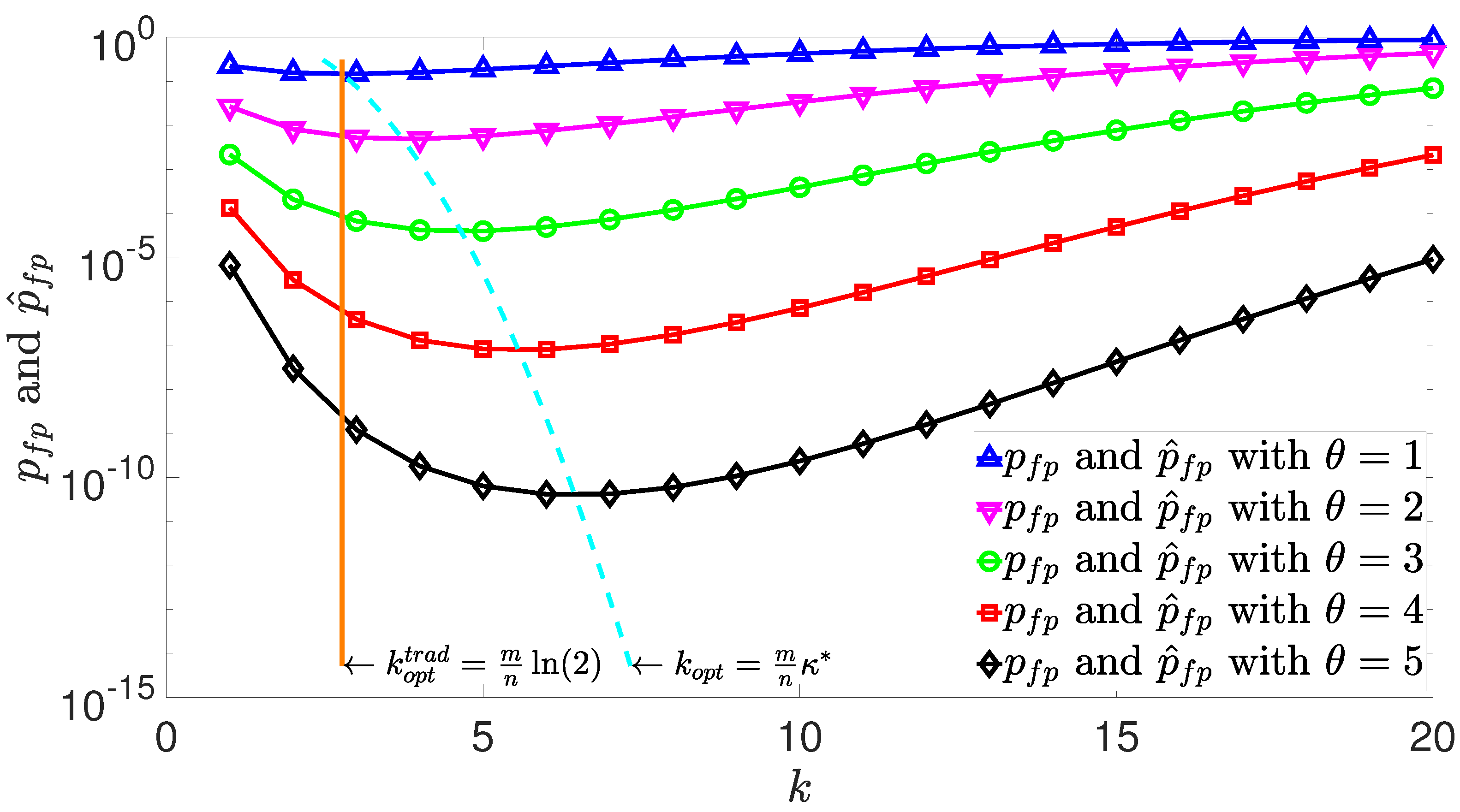
3.1. False Positive Probability

The analysis starts with a derivation of a close approximation for the false positive probability, which is necessary since the exact form given in Equation (2) involves a sum of binomial distributions, which is extremely difficult and time-consuming to compute for large n and m values. For large $x_n$ and small $x_p$, it is well known that a binomial distribution $b(x,x_n,x_p)$ can be approximated by a Poisson distribution with mean $x_n{x}_p$ [20]. For CBF applications, large n (data set size) and m (CBF size) values satisfy these conditions since $x_n=kn$ and $x_p=\frac{1}{m}$. Thus, the approximate false positive probability ${\widehat{p}}_{fp}$ can be written as follows.

$${\widehat{p}}_{fp}(\theta ,k,n,m)={(1-e^{-\frac{kn}{m}}\sum _{l<\theta }\frac{1}{l!}{(\frac{kn}{m})}^l)}^k\approx p_{fp}(\theta ,k,n,m).$$

The cumulative mass function (cmf) of a Poisson distribution is a regularized incomplete gamma function [21]. Thus, the approximate false positive probability can be written as

$${\widehat{p}}_{fp}(\theta ,k,n,m)={\widehat{p}}_{fp}(\theta ,\kappa )={(1-\frac{\mathsf{\Gamma }(\theta ,\kappa )}{\mathsf{\Gamma }(\theta ,0)})}^k,$$

(3)

where the mean of the Poisson distribution used is defined as $\kappa =\frac{kn}{m}$ and $\mathsf{\Gamma }(\theta ,\kappa )={\int }_{\kappa }^{\infty }{t}^{\theta -1}{e}^{-t}\mathrm{d}t.$

As shown in Figure 1, this incomplete Gamma function approximation results in a highly accurate approximation of $p_{fp}$. Note that the approximation ${\widehat{p}}_{fp}$ only depends on the ratio of $kn$ to m. Figure 1 shows that $p_{fp}$ and ${\widehat{p}}_{fp}$ overlap almost 100%. The exact relative error of ${\widehat{p}}_{fp}$ is shown in Figure 2. For the parameters shown, the relative error is less than 0.48% when an optimal number of hash functions is used.

The optimal k values $k_{opt}(\theta )$, for which the false positive probabilities are the lowest, are shown using a dashed cyan line in Figure 1. As can be seen in the figure, $k_{opt}(\theta )$ is definitely not the same, or even close, to $k_{opt}^{trad}(\theta )=k_{opt}(1)$, shown as a solid vertical orange line in Figure 1, when $\theta >1$. Before proposing a systematic method for finding $k_{opt}(\theta )$ for general values of $\theta$, a rigorous analysis will be presented that shows that only one such value exists.

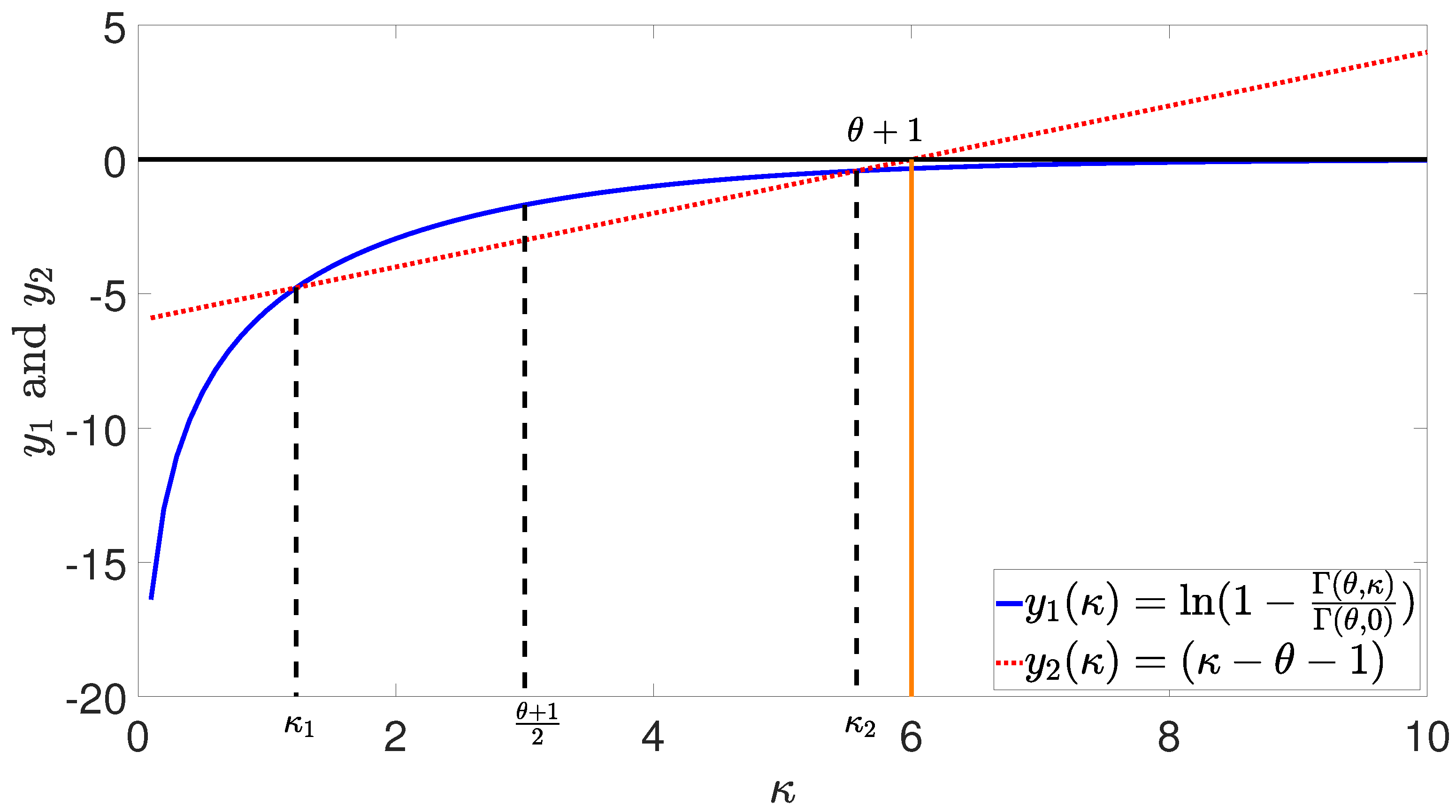
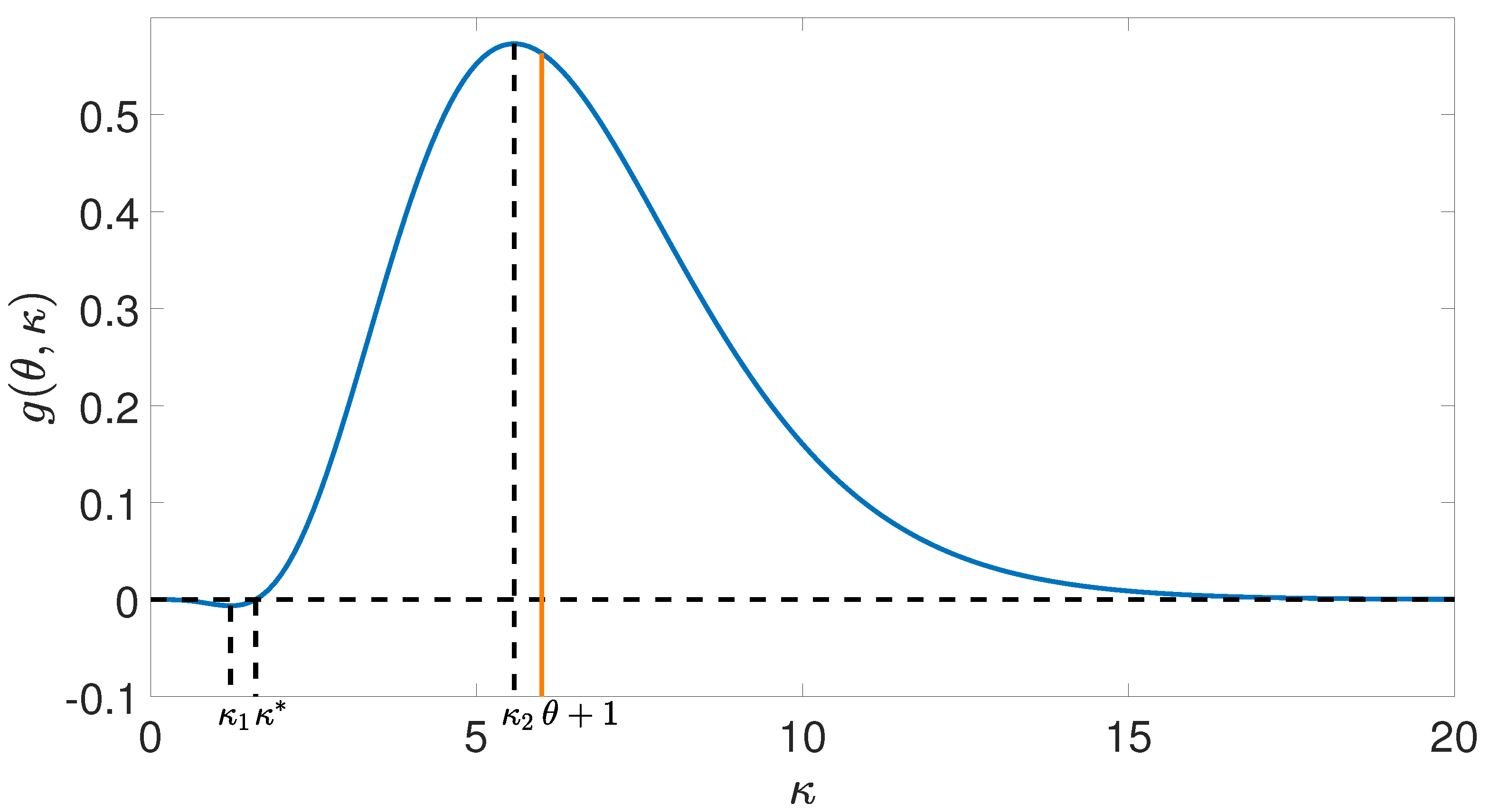
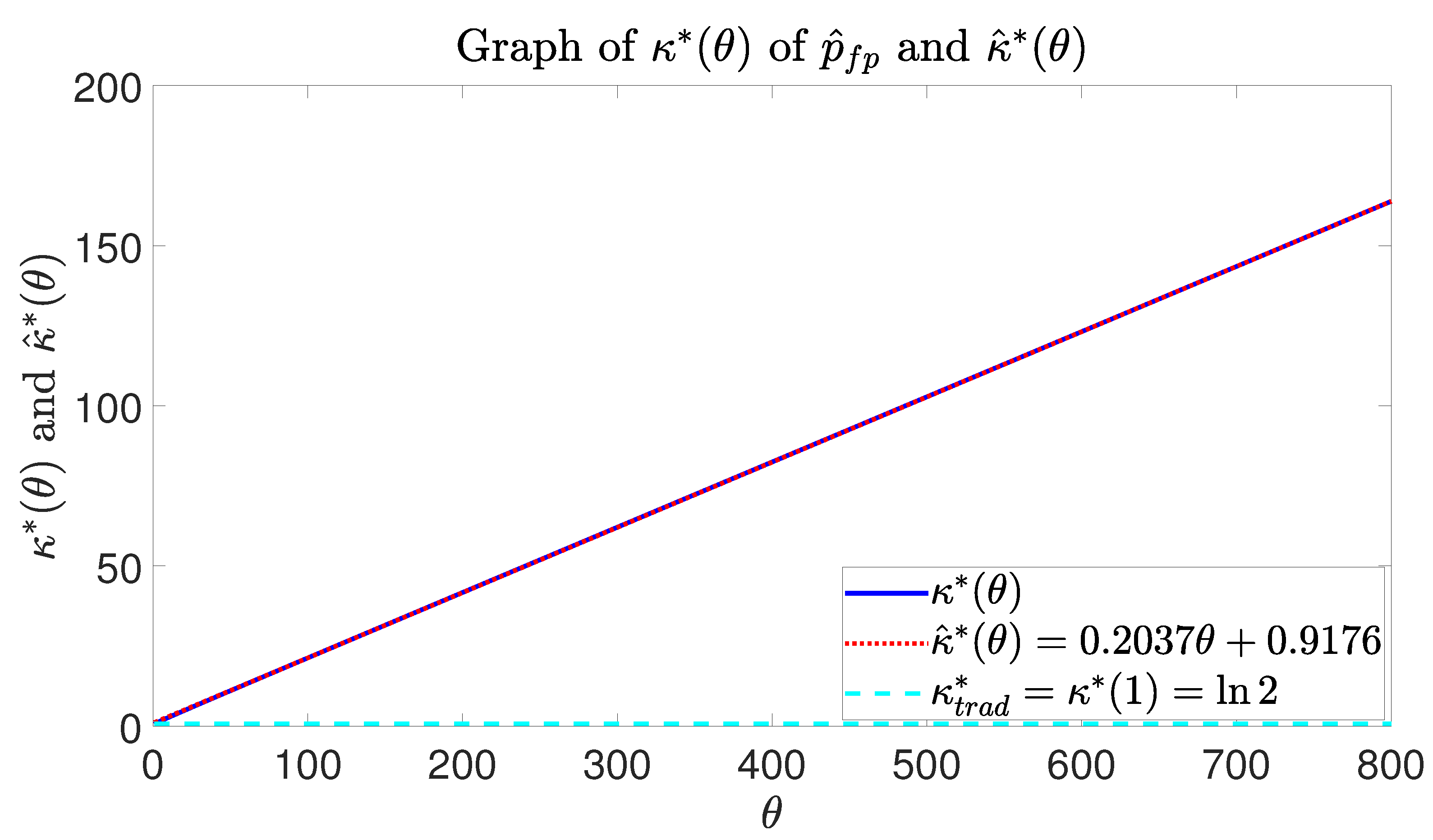
3.2. Uniqueness of Optimal Number of Hash Functions

A sequence of lemmas are used to prove that there exists a unique value of $k_{opt}$ for which the false positive probability is minimized. To follow this proof process, the reader is advised to refer to the plots in Figure 3 and Figure 4 when reading the following lemmas.

Since the optimal false positive probability point occurs when its slope is 0, the proof starts by taking the derivative of ${\widehat{p}}_{fp}(\theta ,k,n,m)$ with respect to k. To find the shape of the derivative of ${\widehat{p}}_{fp}$, the logarithm of ${\widehat{p}}_{fp}$ can be used.

$$ln{\widehat{p}}_{fp}(\theta ,k,n,m)=kln(1-\frac{\mathsf{\Gamma }(\theta ,\kappa )}{\mathsf{\Gamma }(\theta ,0)}).$$

(4)

By taking the derivative of Equation (4),

$$\frac{\frac{\partial }{\partial k}{\widehat{p}}_{fp}(\theta ,k,n,m)}{{\widehat{p}}_{fp}(\theta ,k,n,m)}=ln(1-\frac{\mathsf{\Gamma }(\theta ,\frac{kn}{m})}{\mathsf{\Gamma }(\theta ,0)})+k\frac{\partial }{\partial k}ln(1-\frac{\mathsf{\Gamma }(\theta ,\frac{kn}{m})}{\mathsf{\Gamma }(\theta ,0)}).$$

(5)

By Leibniz’s rule and the definition of the incomplete gamma function [21],

$$\frac{\partial }{\partial k}\mathsf{\Gamma }(\theta ,\frac{kn}{m})=-\frac{n}{m}{(\frac{kn}{m})}^{\theta -1}{e}^{-\frac{kn}{m}}.$$

(6)

Therefore, by applying Equation (6) to the right side of Equation (5) and multiplying both sides of Equation (5) by ${\widehat{p}}_{fp}(\theta ,k,n,m)$,

$$\frac{\partial }{\partial k}{\widehat{p}}_{fp}(\theta ,k,n,m)={\widehat{p}}_{fp}(\theta ,k,n,m)(ln(1-\frac{\mathsf{\Gamma }(\theta ,\frac{kn}{m})}{\mathsf{\Gamma }(\theta ,0)})+\frac{{(\frac{kn}{m})}^{\theta }{e}^{-\frac{kn}{m}}}{\mathsf{\Gamma }(\theta ,0)-\mathsf{\Gamma }(\theta ,\frac{kn}{m})}).$$

For $k_{opt}(\theta )$, this derivative should be set to 0. Since ${\widehat{p}}_{fp}>0$, the second part must be 0. Then, multiplying this second part by a common factor and denoting this term as $g(\theta ,\kappa )$, the following equations and lemmas follow.

$$g(\theta ,\kappa )=(1-\frac{\mathsf{\Gamma }(\theta ,\kappa )}{\mathsf{\Gamma }(\theta ,0)})ln(1-\frac{\mathsf{\Gamma }(\theta ,\kappa )}{\mathsf{\Gamma }(\theta ,0)})+\frac{{\kappa }^{\theta }{e}^{-\kappa }}{\mathsf{\Gamma }(\theta ,0)}$$

To determine whether g is a decreasing or increasing function, the derivative of g is needed.

$$\frac{\partial }{\partial \kappa }g(\theta ,\kappa )=\frac{{\kappa }^{\theta -1}{e}^{-\kappa }}{\mathsf{\Gamma }(\theta ,0)}(1+\theta +ln(1-\frac{\mathsf{\Gamma }(\theta ,\kappa )}{\mathsf{\Gamma }(\theta ,0)})-\kappa ).$$

(7)

In Equation (7), the first part is greater than 0. Thus, g is a decreasing or increasing function depending on the polarity of $1+\theta +ln(1-\frac{\mathsf{\Gamma }(\theta ,\kappa )}{\mathsf{\Gamma }(\theta ,0)})-\kappa$. Let $y_1(\kappa )=ln(1-\frac{\mathsf{\Gamma }(\theta ,\kappa )}{\mathsf{\Gamma }(\theta ,0)})$ and $y_2(\kappa )=(\kappa -\theta -1)$. The $y_1$ and $y_2$ terms are defined in this manner in order to facilitate the examination of the exact conditions under which g is a decreasing or increasing function, and thereby determine the conditions for the changes in slope of the false positive probability function. Then,

$$\frac{\partial }{\partial \kappa }g(\theta ,\kappa )=\frac{{\kappa }^{\theta -1}{e}^{-\kappa }}{\mathsf{\Gamma }(\theta ,0)}(y_1(\kappa )-y_2(\kappa ))$$

Examples of the shapes of $y_1$ and $y_2$ are shown in Figure 3. An example of the $g(\theta ,\kappa )$ function is shown in Figure 4.

Lemma 1.

For a fixed value of θ, $y_1$ is a strictly increasing concave function of κ.

Proof of Lemma 1.

Using the definition of an incomplete Gamma function, the first partial derivative of $y_1$ can be shown to be greater than zero. i.e.,

$$\frac{\partial y_1}{\partial \kappa }=\frac{{\kappa }^{\theta -1}}{e^{\kappa }(\mathsf{\Gamma }(\theta ,0)-\mathsf{\Gamma }(\theta ,\kappa ))}>0$$

Then, using the second partial derivative, it can also be verified that $y_1$ is concave when $\kappa \ge \theta -1$.

$$\frac{{\partial }^2{y}_1}{\partial {\kappa }^2}=\frac{{\kappa }^{\theta -2}\mathsf{\Gamma }(\theta ,0)}{e^{\kappa }}\frac{(\theta -1-\kappa )(1-\frac{\mathsf{\Gamma }(\theta ,\kappa )}{\mathsf{\Gamma }(\theta ,0)})-\frac{{\kappa }^{\theta }{e}^{-\kappa }}{\mathsf{\Gamma }(\theta ,0)}}{{(\mathsf{\Gamma }(\theta ,0)-\mathsf{\Gamma }(\theta ,\kappa ))}^2}.$$

(8)

Now consider the situation when $\kappa <\theta -1$. The following are well-known properties of a Poisson distribution with mean $\kappa$, denoted by $Po{i}_{\kappa }(X=\theta )$ [22],

$$Po{i}_{\kappa }(X=\theta )<Po{i}_{\kappa }(X\ge \theta )<\frac{Po{i}_{\kappa }(X=\theta )}{1-\frac{\kappa }{\theta +1}}.$$

(9)

Then, based on [21] and applying Equation (9) to $(\theta -1-\kappa )(1-\frac{\mathsf{\Gamma }(\theta ,\kappa )}{\mathsf{\Gamma }(\theta ,0)})-\frac{{\kappa }^{\theta }{e}^{-\kappa }}{\mathsf{\Gamma }(\theta ,0)}$ in Equation (8),

$$(\theta -1-\kappa )Po{i}_{\kappa }(X\ge \theta )-\theta Po{i}_{\kappa }(X=\theta )<(\frac{\theta -1-\kappa }{1-\frac{\kappa }{\theta +1}}-\theta )Po{i}_{\kappa }(X=\theta )<-\frac{1+\kappa +\theta }{\theta +1-\kappa }Po{i}_{\kappa }(X=\theta )<0.$$

Thus, $\frac{{\partial }^2{y}_1}{\partial {\kappa }^2}<0$ when $\kappa <\theta -1$. Therefore, $y_1$ is a strictly increasing concave function for all values of $\kappa$. □

Lemma 2.

$y_1(\kappa =\frac{\theta +1}{2})>y_2(\kappa =\frac{\theta +1}{2})$

Proof of Lemma 2.

Lemma 2 is equivalent to

$$\frac{\theta +1}{2}+ln(1-\frac{\mathsf{\Gamma }(\theta ,\frac{\theta +1}{2})}{\mathsf{\Gamma }(\theta ,0)})>0.$$

From [21], by putting $\frac{\theta +1}{2}$ into the $ln()$ function,

$$ln(\sum _{l\ge \theta }\frac{{(\frac{\theta +1}{2})}^l}{l!})>0,$$

which is equivalent to

$$\sum _{l\ge \theta }\frac{{(\frac{\theta +1}{2})}^l}{l!}>1.$$

(10)

Then, by the Stirling inequality,

$$\frac{{(\frac{\theta +1}{2})}^{\theta }}{\theta !}\ge \frac{1}{e\sqrt{\theta }}{(\frac{e}{\theta })}^{\theta }{(\frac{\theta +1}{2})}^{\theta }=\frac{1}{e\sqrt{\theta }}{(\frac{e}{2})}^{\theta }{(1+\frac{1}{\theta })}^{\theta }.$$

The function on the right hand side decreases from $\theta =0$ to 1 and increases from $\theta =1$ to ∞. The minimum value of this function is 1, which occurs at some point $\theta$ with $\theta >0$. Thus, $\frac{{(\frac{\theta +1}{2})}^{\theta }}{\theta !}\ge 1.$ Therefore, ${\displaystyle \sum _{l\ge \theta }}\frac{{(\frac{\theta +1}{2})}^l}{l!}>\frac{{(\frac{\theta +1}{2})}^{\theta }}{\theta !}\ge 1.$ □

Lemma 3.

$\underset{\kappa \to 0^{+}}{lim}g(\theta ,\kappa )=0$, and $g(\theta ,\kappa )$ is a strictly decreasing function for $\kappa \in (0,{\kappa }_1)$, where ${\kappa }_1\in (0,\frac{\theta +1}{2})$.

Proof of Lemma 3.

From L’Hopital’s rule, $\underset{x\to 0^{+}}{lim}xlnx=0$. This implies that $\underset{\kappa \to 0^{+}}{lim}(1-\frac{\mathsf{\Gamma }(\theta ,\kappa )}{\mathsf{\Gamma }(\theta ,0)})ln(1-\frac{\mathsf{\Gamma }(\theta ,\kappa )}{\mathsf{\Gamma }(\theta ,0)})=0$. Therefore, $\underset{\kappa \to 0^{+}}{lim}g(\theta ,\kappa )=0$.

As $\kappa$ approaches 0 from the right, $\underset{\kappa \to 0^{+}}{lim}{y}_1(\kappa )=-\infty$, and $\underset{\kappa \to 0^{+}}{lim}{y}_2(\kappa )=-\theta -1$. This implies that $\underset{\kappa \to 0^{+}}{lim}{y}_1(\kappa )<\underset{\kappa \to 0^{+}}{lim}{y}_2(\kappa )$. On the other hand, by Lemma 2, $y_1(\kappa =\frac{\theta +1}{2})>y_2(\kappa =\frac{\theta +1}{2})$. Therefore, by the intermediate value theorem, there exists a point ${\kappa }_1\in (0,\frac{\theta +1}{2})$ that satisfies $y_1({\kappa }_1)=y_2({\kappa }_1)$. Then, since $y_1({\kappa }_1)<y_2(\kappa )$ as $\kappa \to 0^{+}$, $y_2$ is a straight line, and Lemma 1 states that $y_1$ is a strictly increasing function of $\kappa$, $y_1(\kappa )<y_2(\kappa )$ for $\kappa \in (0,{\kappa }_1)$. Thus, $\frac{\partial }{\partial \kappa }g(\theta ,\kappa )<0$ for $\kappa \in (0,{\kappa }_1)$. □

Lemma 4.

The function $g(\theta ,\kappa )$ is a strictly increasing function for $\kappa \in ({\kappa }_1,{\kappa }_2)$, where $\frac{\theta +1}{2}<{\kappa }_2<\theta +1$.

Proof of Lemma 4.

From Lemma 2 again, $y_1(\kappa =\frac{\theta +1}{2})>y_2(\kappa =\frac{\theta +1}{2})$. On the other hand, for all real positive values $\kappa$, $y_1(\kappa )<0$, whereas $y_2(\theta +1)=0$. Thus, $y_1(\theta +1)<y_2(\theta +1)$. Therefore, by the intermediate value theorem again, there is a point $\frac{\theta +1}{2}<{\kappa }_2<\theta +1$ that satisfies $y_1({\kappa }_2)=y_2({\kappa }_2)$. Finally, in the interval of $\kappa \in ({\kappa }_1,{\kappa }_2)$, $\frac{\partial }{\partial \kappa }g(\theta ,\kappa )>0$ because $y_1(\kappa )>y_2(\kappa )$ in this interval. □

Lemma 5.

The function $g(\theta ,\kappa )$ is a strictly decreasing function for $\kappa \in ({\kappa }_2,\infty )$, and $\underset{\kappa \to \infty }{lim}g(\theta ,\kappa )=0$.

Proof of Lemma 5.

By the definition of an incomplete gamma function, $\mathsf{\Gamma }(\theta ,\kappa )={\int }_{\kappa }^{\infty }{t}^{\theta -1}{e}^{-t}\mathrm{d}t$, the limit of $\mathsf{\Gamma }(\theta ,\kappa )$ as $\kappa$ approaches positive infinity is 0. This makes the left term of $g(\theta ,\kappa )$ become $1ln1=0$ when $\kappa$ approaches positive infinity. The right term becomes 0 by L’Hopital’s rule. Therefore, $\underset{\kappa \to \infty }{lim}g(\theta ,\kappa )=0$. From Lemma 1, $y_1$ is strictly concave, and from the proof of Lemma 4, $y_1({\kappa }_2)=y_2({\kappa }_2)$. Thus, for $\kappa >{\kappa }_2$, $\frac{\partial }{\partial \kappa }g(\theta ,\kappa )<0$ because $y_1(\kappa )<y_2(\kappa )$. □

Theorem 1.

Given n, m and a count threshold $\theta >0$, there exists a unique value $k=k_{opt}$ for which the false positive probability of a CBF has the minimum value. Furthermore, $k_{opt}(\theta )=\lfloor \frac{m}{n}{\kappa }^{*}(\theta )\rfloor$ or $k_{opt}(\theta )=\lceil \frac{m}{n}{\kappa }^{*}(\theta )\rceil$.

Proof of Theorem 1.

In the interval of $\kappa \in (0,{\kappa }_1]$, $g(\theta ,\kappa )<0$ due to Lemma 3. Also, $g(\theta ,{\kappa }_2)>0$ because Lemma 5 states that $g(\theta ,\kappa )$ is a strictly decreasing function from ${\kappa }_2$ to ∞, at which point $g(\theta ,\kappa )$ approaches zero. Then, due to Lemma 4, there is a unique value ${\kappa }^{*}\in ({\kappa }_1,{\kappa }_2)$ such that $g(\theta ,{\kappa }^{*})=0$. Finally, using the definition of $\kappa$, the theorem follows. □

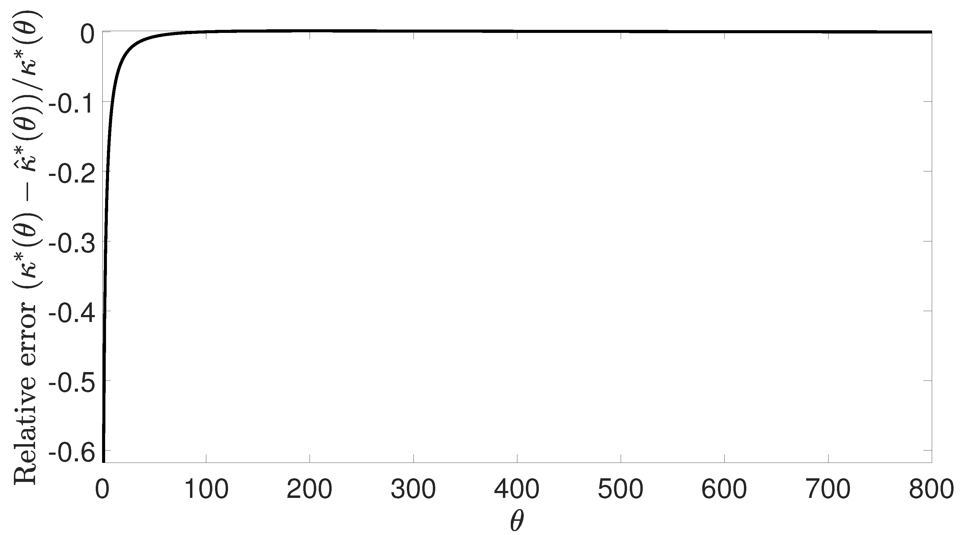
3.3. Procedure for Determining the Optimal Number of Hash Functions

Based on the lemmas and theorem of the previous subsection, a general procedure to be used to find the optimal number of hash functions $k_{opt}(\theta )$ is as follows. Start from $k=1$ and compute the false positive probability ${\widehat{p}}_{fp}^{*}(\theta ,k,n,m)$ using Equation (3). Then increment k by one and recompute the false positive probability. Continue until the false positive probability starts to increase or $k=(\theta +1)n/m$, whichever comes first. The k value that results in the minimum ${\widehat{p}}_{fp}^{*}(\theta ,k,n,m)$ is $k_{opt}(\theta )$.

The above procedure can be simplified by using precomputed tables or a linear approximation.

Table 1. The ${\kappa }^{*}(\theta )$, ${\widehat{\kappa }}^{*}(\theta )$, and relative error between ${\kappa }^{*}(\theta )$ and ${\widehat{\kappa }}^{*}(\theta )$ values.

$\mathit{\theta }$	${\mathit{\kappa }}^{*}(\mathit{\theta })$	${\widehat{\mathit{\kappa }}}^{*}(\mathit{\theta })$	$\frac{{\mathit{\kappa }}^{*}(\mathit{\theta })-{\widehat{\mathit{\kappa }}}^{*}(\mathit{\theta })}{{\mathit{\kappa }}^{*}(\mathit{\theta })}$	$\mathit{\theta }$	${\mathit{\kappa }}^{*}(\mathit{\theta })$	${\widehat{\mathit{\kappa }}}^{*}(\mathit{\theta })$	$\frac{{\mathit{\kappa }}^{*}(\mathit{\theta })-{\widehat{\mathit{\kappa }}}^{*}(\mathit{\theta })}{{\mathit{\kappa }}^{*}(\mathit{\theta })}$	$\mathit{\theta }$	${\mathit{\kappa }}^{*}(\mathit{\theta })$	${\widehat{\mathit{\kappa }}}^{*}(\mathit{\theta })$	$\frac{{\mathit{\kappa }}^{*}(\mathit{\theta })-{\widehat{\mathit{\kappa }}}^{*}(\mathit{\theta })}{{\mathit{\kappa }}^{*}(\mathit{\theta })}$
1	0.6931	1.1213	−0.6177	11	2.9099	3.1583	−0.0854	21	5.0183	5.1953	−0.0353
2	0.9326	1.3250	−0.4207	12	3.1228	3.3620	−0.0766	22	5.2274	5.3990	−0.0328
3	1.1635	1.5287	−0.3139	13	3.3351	3.5657	−0.0691	23	5.4362	5.6027	−0.0306
4	1.3893	1.7324	−0.2469	14	3.5469	3.7694	−0.0627	24	5.6448	5.8064	−0.0286
5	1.6117	1.9361	−0.2013	15	3.7582	3.9731	−0.0572	25	5.8533	6.0101	−0.0268
6	1.8317	2.1398	−0.1682	16	3.9690	4.1768	−0.0524	26	6.0616	6.2138	−0.0251
7	2.0498	2.3435	−0.1433	17	4.1795	4.3805	−0.0481	27	6.2697	6.4175	−0.0236
8	2.2664	2.5472	−0.1239	18	4.3896	4.5842	−0.0443	28	6.4776	6.6212	−0.0222
9	2.4818	2.7509	−0.1084	19	4.5995	4.7879	−0.0410	29	6.6854	6.8249	−0.0209
10	2.6963	2.9546	−0.0958	20	4.8090	4.9916	−0.0380	30	6.8931	7.0286	−0.0197

shows a table of precomputed optimal ${\kappa }^{*}$ values for count thresholds $\theta$ ranging from 1 to 30. This table was created by following the procedure outlined above. Since $\kappa =kn/m$, this table can be used to determine $k_{opt}$ by simply using the relationship shown in Theorem 1; i.e., $k_{opt}$ is either the floor or ceiling of ${\kappa }^{*}m/n$.

For large count thresholds $\theta$, a straight line approximation can be used to determine ${\kappa }^{*}$, and thereby $k_{opt}$. Figure 5 shows that the straight line approximation

$${\widehat{\kappa }}^{*}(\theta )=0.2037\theta +0.9176$$

(11)

closely tracks ${\kappa }^{*}(\theta )$ for large $\theta$ values. By plotting the relative errors, as shown in Figure 6, it can be seen that there is a relative error of less than about 2 percent when $\theta >30$.

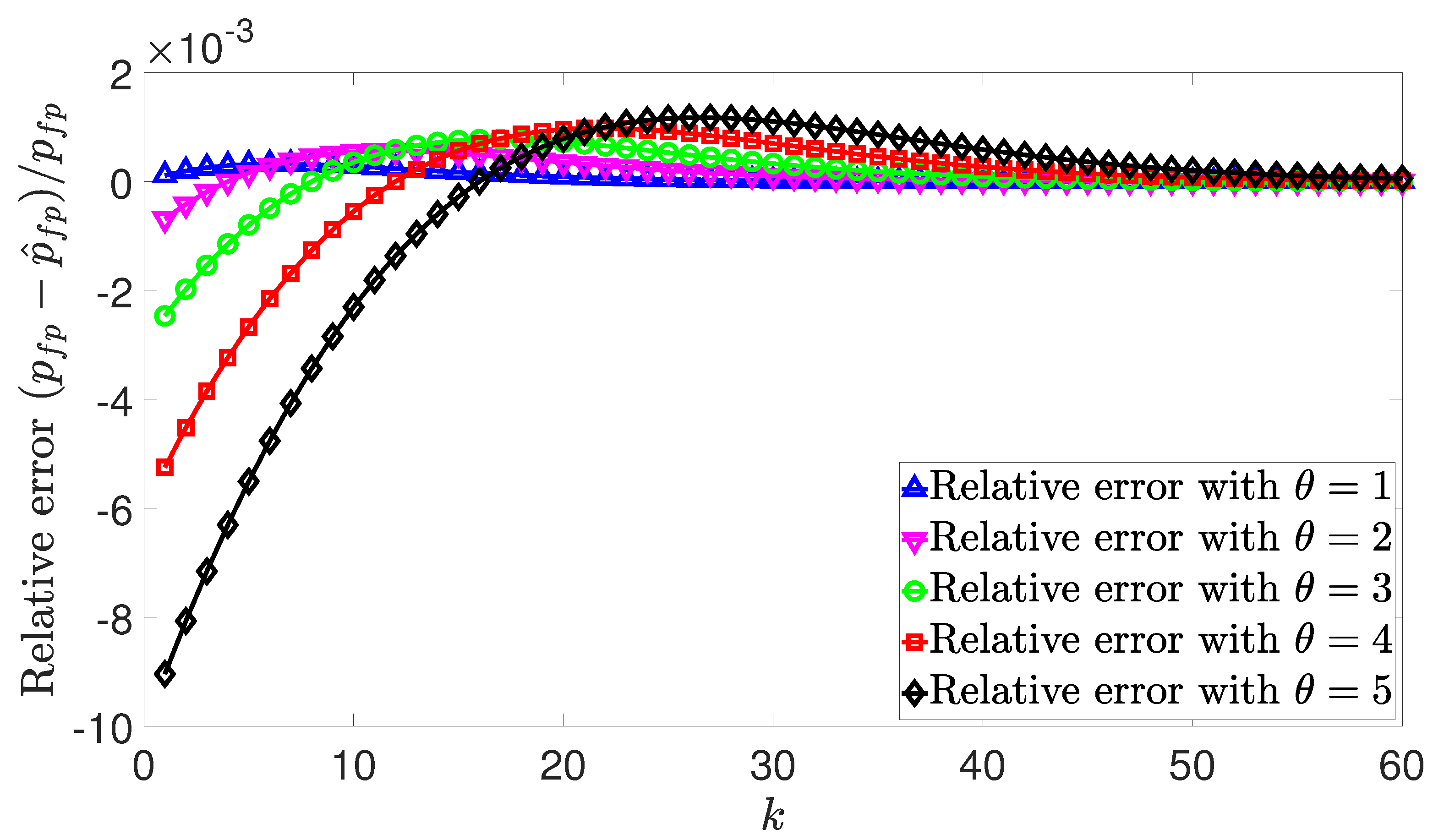
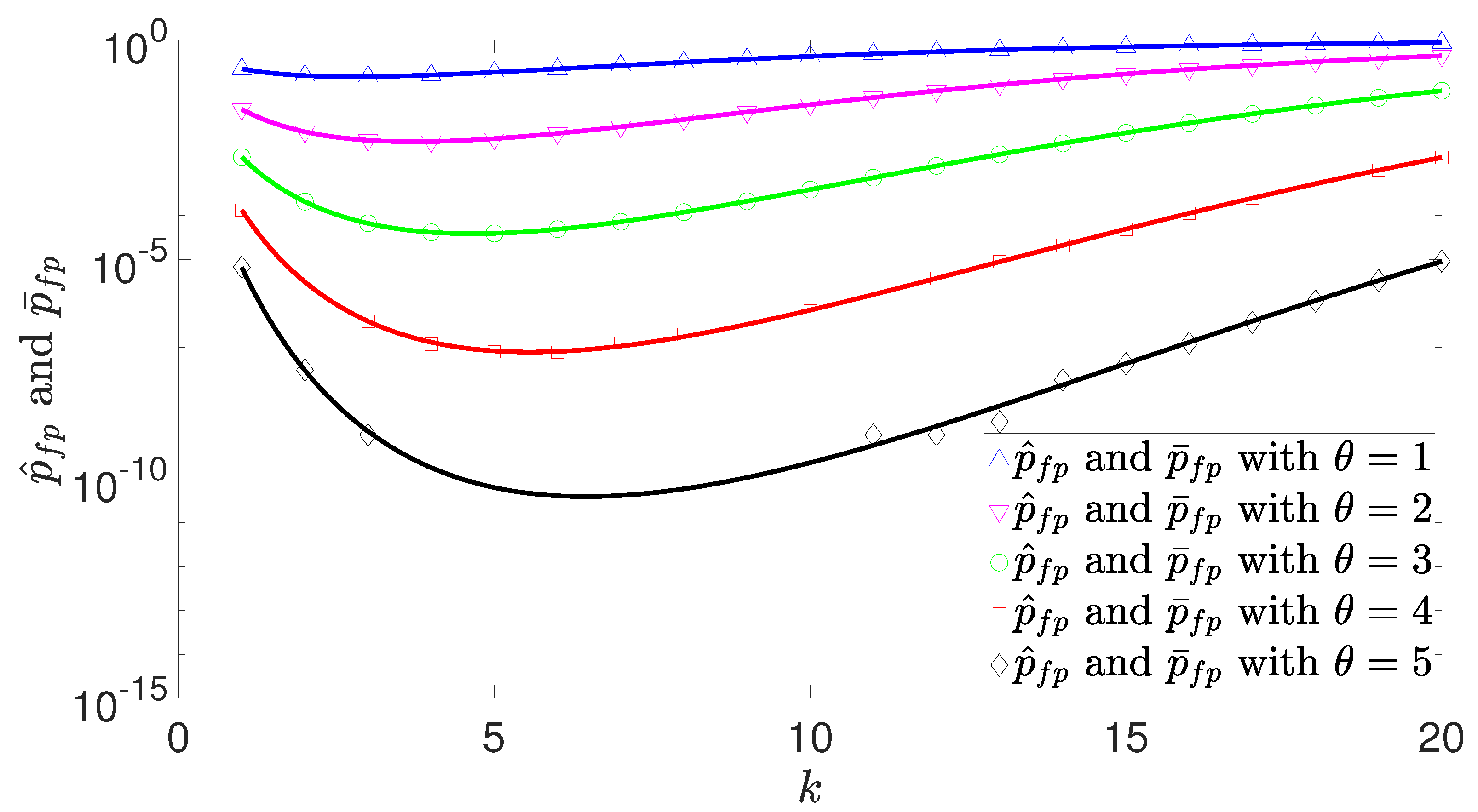
4. Simulation Results

Simulations were conducted to verify the proposed theoretical analysis. A simulation program was written in Java for a general CBF with n data entries, m CBF elements, and k hash functions. The hash functions were created as uniform random distributions between 0 and $m-1$ using the pseudorandom number generator provided in the java.util.Random package and stored in tables so that they could be reused during hashing. Care was taken to ensure that the hash functions created were orthogonal to each other. This simulator program is freely available for all interested readers.

Figure 7 shows the false positive simulation results obtained with an example set of n, m, and count threshold $\theta$ values. The open triangle, circle, square, and diamond marks refer to the simulation results ${\overline{p}}_{fp}$ while the solid curves show the expected false positive probabilties ${\widehat{p}}_{fp}$.

Each simulation result, which was the average of 100 simulation runs, was obtained in the following manner. The CBF was initialized by setting all m CBF entries to 0. Then, n data entries were generated randomly. For each data entry, k hash functions, applied by looking up table values from precomputed random hashes (as described above), are applied and used to increment the CBF entries corresponding to the hash function outputs. Finally, $n_q=n$ queries were randomly generated and the k hash functions are applied to each of those queries. Each query resulted in a “true” answer if all k CBF elements mapped by the k hash functions are greater than or equal to the count threshold $\theta$. Finally, the number of false positives generated in this manner were counted and divided by $n_q$ to produce the false positive probability.

Figure 7 shows the false positive rate simulation and analysis results, as a function of k, with $n=10$ million, $m=40$ million, and $\theta$ values ranging from 1 to 5. As can be seen from the figure, the simulation results closely map the theoretical results, with slight variations only visible for exceedingly low false probabilities of ${10}^{-7}$ or smaller. Exceedingly low false probabilities imply rare occurrences of false positives, thus requiring longer simulation runs to obtain accurate results. Even lower false positive probabilities (smaller than ${10}^{-9}$) then result in zero occurrences of false positive events in our simulations. Thus, simulation results were not recorded, since false positive events did not occur, for $\theta =5$ and $k=4$ through 10 in Figure 7.

5. Conclusions

This paper has investigated the problem of determining the optimal parameter values to be used for counting bloom filters used in applications requiring approximate count thresholds. Rigorous analysis has led to a highly accurate equation for the false positive probability, with relative errors of less than 0.48% given typical parameter values. It has also been proven that there exists a unique number of hash functions $k_{opt}$ for which an minimal false positive probability is obtained. Next, a systematic procedure based on precomputed tables and a linear approximation has been presented for finding $k_{opt}$. Finally, realistic simulations modeling the use of a CBF for a count thresholding application has been used to show that the theoretical analysis closely models actual CBF behavior.

References

1. Bloom, B.H. Space/time trade-offs in hash coding with allowable errors. Commun. ACM 1970, 13, 422–426. [Google Scholar] [CrossRef]
2. Guo, D.; Liu, Y.; Li, X.; Yang, P. False negative problem of counting bloom filter. IEEE Trans. Knowl. Data Eng. 2010, 22, 651–664. [Google Scholar]
3. Ghosh, M.; Ozer, E.; Ford, S.; Biles, S.; Lee, H.H.S. Way Guard: A segmented counting Bloom filter approach to reducing energy for set-associative caches. In Proceedings of the International Symposium on Low Power Electronics and Design (ISPLED), San Fancisco, CA, USA, 19–21 August 2009; pp. 165–170. [Google Scholar]
4. Yun, J.; Lee, S.; Yoo, S. Dynamic wear leveling for phase-change memories with endurance variations. IEEE Trans. Very Large Scale Integr. (VLSI) Syst. 2015, 23, 1604–1615. [Google Scholar] [CrossRef]
5. Maggs, B.M.; Sitaraman, R.K. Algorithmic nuggets in content delivery. ACM SIGCOMM Comput. Commun. Rev. 2015, 45, 52–66. [Google Scholar] [CrossRef]
6. Lu, Y.; Montanari, A.; Prabhakar, B.; Dharmapurikar, S.; Kabbani, A. Counter braids: A novel counter architecture for per-flow measurement. ACM SIGMETRICS Perform. Eval. Rev. 2008, 36, 121–132. [Google Scholar] [CrossRef]
7. Bonomi, F.; Mitzenmacher, M.; Panigrah, R.; Singh, S.; Varghese, G. Beyond bloom filters: From approximate membership checks to approximate state machines. In Proceedings of the ACM SIGCOMM 2006 Conference on Applications, Technologies, Architectures, and Protocols for Computer Communications, Pisa, Italy, 11–15 September 2006; Volume 36, pp. 315–326. [Google Scholar]
8. Dharmapurikar, S.; Krishnamurthy, P.; Taylor, D.E. Longest prefix matching using bloom filters. In Proceedings of the 2003 Conference on Applications, Technologies, Architectures, and Protocols for Computer Communications, Karlsruhe, Germany, 25–29 August 2003; pp. 201–212. [Google Scholar]
9. Song, H.; Hao, F.; Kodialam, M.; Lakshman, T. Ipv6 lookups using distributed and load balanced bloom filters for 100gbps core router line cards. In Proceedings of the IEEE INFOCOM 2009, Rio de Janeiro, Brazil, 19–25 April 2009; pp. 2518–2526. [Google Scholar]
10. Ficara, D.; Di Pietro, A.; Giordano, S.; Procissi, G.; Vitucci, F. Enhancing counting Bloom filters through Huffman-coded multilayer structures. IEEE/ACM Trans. Netw. (TON) 2010, 18, 1977–1987. [Google Scholar] [CrossRef]
11. Fan, L.; Cao, P.; Almeida, J.; Broder, A.Z. Summary cache: A scalable wide-area web cache sharing protocol. IEEE/ACM Trans. Netw. (TON) 2000, 8, 281–293. [Google Scholar] [CrossRef]
12. Chazelle, B.; Kilian, J.; Rubinfeld, R.; Tal, A. The Bloomier filter: An efficient data structure for static support lookup tables. In Proceedings of the Fifteenth Annual ACM-SIAM Symposium on Discrete Algorithms. Society for Industrial and Applied Mathematics, New Orleans, LA, USA, 11–14 January 2004; pp. 30–39. [Google Scholar]
13. Moraru, I.; Andersen, D.G. Exact pattern matching with feed-forward bloom filters. J. Exp. Algorithm. (JEA) 2012, 17, 3–4. [Google Scholar] [CrossRef]
14. Ho, J.T.L.; Lemieux, G.G. PERG: A scalable FPGA-based pattern-matching engine with consolidated bloomier filters. In Proceedings of the 2008 IEEE International Conference on Field-Programmable Technology, Taipei, Taiwan; 2008; pp. 73–80. [Google Scholar]
15. Melsted, P.; Pritchard, J.K. Efficient counting of k-mers in DNA sequences using a bloom filter. BMC Bioinform. 2011, 12, 333. [Google Scholar] [CrossRef] [PubMed]
16. Sun, C.; Fan, J.; Shi, L.; Liu, B. A novel router-based scheme to mitigate SYN flooding DDoS attacks. IEEE INFOCOM (Student Poster). 2007. Available online: https://pdfs.semanticscholar.org/fdae/7b20d220a1c23f9f6c0f8464574f78ef55c0.pdf (accessed on 11 July 2019).
17. Tarkoma, S.; Rothenberg, C.E.; Lagerspetz, E. Theory and Practice of Bloom Filters for Distributed Systems. IEEE Commun. Surv. Tutor. 2012, 14, 131–155. [Google Scholar] [CrossRef]
18. Broder, A.; Mitzenmacher, M. Network Applications of Bloom Filters: A Survey. Int. Math. 2003, 1, 485–509. [Google Scholar] [CrossRef]
19. Mitzenmacher, M.; Upfal, E. Probability and Computing: Randomized Algorithms and Probabilistic Analysis; Cambridge University Press: Cambridge, UK, 2005. [Google Scholar]
20. Papoulis, A.; Pillai, S.U. Probability, Random Variables, and Stochastic Processes; Tata McGraw-Hill Education: Pennsylvania Plaza, NY, USA, 2002; pp. 55–57. [Google Scholar]
21. Abramowitz, M.; Stegun, I. Handbook of Mathematical Functions: With Formulas, Graphs, and Mathematical Tables Applied Mathematics Series; National Bureau of Standards: Gaithersburg, MD, USA, 1964; pp. 260–265.
22. Klar, B. Bounds on tail probabilities of discrete distributions. Probab. Eng. Inf. Sci. 2000, 14, 161–171. [Google Scholar] [CrossRef]
Figure 1. Plot of false positive probabilities with θ = 1 to θ = 5 vs. the number of hash functions k. The ratio m / n is set to four and the cyan dashed line shows k o p t ( θ ) . The sample points correspond to p f p and the lines correspond to p ^ f p . The two functions overlap almost 100 percent.
Electronics 08 00779 g001
Figure 2. Plot of relative error between exact and approximate false positive probabilities with θ = 1 to θ = 5 vs. the number of hash functions k. n = 1000 and m = 4000 are used in this plot, and larger values of n and m result in slightly lower relative errors.
Electronics 08 00779 g002
Figure 3. A plot showing y 1 and y 2 , used in Lemmas 1 and 2, as a function of κ for θ = 5 .
Electronics 08 00779 g003
Figure 4. g ( θ , κ ) as a function of κ for θ = 5 and m / n = 4 . κ 1 1.2262 , κ 2 5.5756 < 6 , and κ * 1.6117 .
Electronics 08 00779 g004
Figure 5. The functions κ * ( θ ) and κ ^ * ( θ ) as a function of θ .
Electronics 08 00779 g005
Figure 6. Plot of relative error between κ * ( θ ) and κ ^ * ( θ ) vs. θ .
Electronics 08 00779 g006
Figure 7. Plot of false positive theoretical values ( p ^ f p ) and simulation results ( p ¯ f p ) where n = 10,000,000, m = 40,000,000, θ = 1 , 2 , 3 , 4 , 5 , and n q = n vs. k between 1 to 20.
Electronics 08 00779 g007