Abstract
Infrared imaging is widely applied in the discrimination of spatial targets. Extracting distinguishable features from the infrared signature of spatial targets is an important premise for this task. When a target in outer space experiences micro-motion, it causes periodic fluctuations in the observed infrared radiation intensity signature. Periodic fluctuations can reflect some potential factors of the received data, such as structure, dynamics, etc., and provide possible ways to analyze the signature. The purpose of this paper is to estimate the micro-motion dynamics and geometry parameters from the observed infrared radiation intensity signature. To this end, we have studied the signal model of the infrared radiation intensity signature, conducted the geometry and micro-motion models of the target, and we proposed a joint parameter estimation method based on optimization techniques. After analyzing the estimation results, we testified that the parameters of micro-motion and geometrical shape of the spatial target can be effectively estimated by our estimation method.
1. Introduction
Spatial target recognition is a significant problem in many scientific and engineering fields, such as precise guidance systems and space surveillance systems. Infrared imaging technology is widely used in spatial target recognition systems. On account of the long distance between the target and sensor, spatial targets are often shown as a single pixel on the infrared image, which is a great challenge with respect to recognition. The grey level in infrared images of the objects varies with time, called the infrared signature, which contains numerous information and can be used in discrimination and tracking systems. In the past few decades, a large number of analysis methods have been utilized. Resch implemented exoatmosphere object recognition using an extracted feature, the ratios of the object’s irradiance, and the time-averaged irradiance values of each object in the FOV (field of view) [1].
A spatial target may have micro-motions due to maneuvering control or uneven force during exoatmospheric flight, such as tumbling, spinning, and precessing [2]. Estimating micro-motion parameters of objects has received attention in the radar community as well. An analysis method based on mixed micro-Doppler time-frequency sequences has been put forward to extract micro-motion dynamic and inertial characteristics of free rigid targets in space [3]. However, radar signals are susceptible to interference and application scenarios are limited.
This prompted us to study infrared signals for the analysis and extraction of spatial target micro-motion features. If the target experiences some micro-motion, the feature of the target projection area is typically a time-varying amplitude function and periodically time-varying modulation is applied to the received IR signal [4]. Therefore, from the accurate mathematical description of the observed infrared signature, it is feasible to obtain the complete signal of the target projection area and estimate the micro-motion parameters (including the spin rate, the precession rate, and the nutation angle, etc.) and geometric parameters that are not available for the signal without micro-motion. Deng [5] studied the influence of inertial parameters, including inertial moments (MOI) and initial angular rate (IAR) on the target infrared radiation sequence, without considering the rich target information contained in parameters, such as precession angle and shape parameters. Liu [6] used a sparse representation method for micro-motion parameter estimation. The problem of sparse representation is suitable to be solved by the "relaxed" convex optimization method, and the regularization parameters are introduced. However, this method is limited to the case targets having sparse features, and it does not have universal adaptability.
This paper develops a projection model of spatial targets and derives mathematical formulas of projection area signatures induced by micro-motions. We also propose a joint parameter estimation method with optimization techniques of target micro-motion dynamics and geometrical shape parameters from IR intensity features, which makes it easier to extract useful information when constructing classifiers or other predictors in IR space applications. And our method is applicable to situations where the shape of the target is not limited.
The rest of the paper is organized as follows: A signature model is constructed in Section 2 and a simulation has been conducted. A shape estimation algorithm and experiments are put forward in Section 3, followed by a joint estimation algorithm and experiments in Section 4. Conclusions are presented in the last section.
2. Infrared Signature Model
For infrared detection of outer space targets, the infrared energy received by the detector is only from the radiation of the target and the deep space of the universe if we keep stars (sun, moon, and etc.) out of the FOV. The radiation deep in outer space is small and negligible. The radiation of the target is determined by temperature, infrared emissivity, projection area, observing angle, and so on.
2.1. Emitted Radiation Analysis
The blackbody is an idealized model. Eb(λ,T) is the spectral radiant existence of a blackbody in the waveband λ1–λ2 at an absolute temperature T, which is defined by Plank’s radiation law [7] as:
where c1 represents the first radiation constant with the value of is 3.7419 × 10⁻¹⁶ W·m2, c2 denotes the second radiation constant, and the value is 1.4388 × 10⁻² m·K.
Suppose AO and φ are the entrance pupil area of sensor and the angle between the principle axis of the lens and LOS (line of sight), RS denotes the distance from the object to the sensor, and Aproj is the projecting area of the object at LOS, and ε is the surface material or coating infrared emissivity of the target, the whole radiation power Ie received by the observing sensor for an exo-atmospheric object in the waveband λ1–λ2 at an absolute temperature T is approximately represented as:
2.2. Target Geometry Model
Assume that the convex target surface is divided into N small triangles, its area and the normal vector are ai and ni (i = 1, ..., N), respectively, and the vector of line of sight is nLOS. Due to the convex surface on the topology, relation among triangles in any cover phenomenon does not exist, and the target projection area is an accumulation of all triangles’ projection areas in the detection field [8]. The target projection area Aproj can be expressed as:
where n′LOS is detecting line of sight in the local coordinate system.
For the sake of simplicity, this paper takes the cone object as an example. Figure 1 shows the geometry structure of the cone object and LOS in the local coordinate system. The projecting area of the object at the LOS orientation can be computed by following integration:
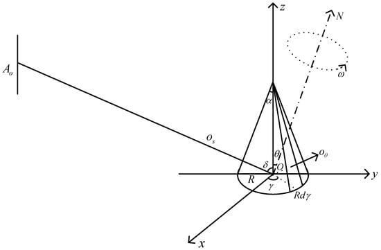
Figure 1.
Projection area model of the cone object.
In the formula, α represents the cone object’s half angle, R is the circle radius of the cone’s bottom, is the unit normal vector of the conical region, is the bottom unit normal vector, and is the unit direction vector of LOS, where φ expresses the azimuth angle of LOS. Therefore the computing result of projection area is:
According to above analysis, we discovered that the projection area at the sensor orientation is only related to the angle δ on condition that given the cone.
2.3. Attitude Motion Model
Exoatmospheric targets are mainly influenced by gravity, and their flight attitude is not fixed with changing period. There are three main motion types, including spinning, tumbling, and precession in terms of spatial targets. Different motion types leads to difference in the infrared signature of targets [9]. The attitude and position have important effects on the signal. Therefore, the observing angle from the sensor to the target is studied.
Suppose the motion type of the target is precessing and spinning. The variation mode of δ is addressed in the following part. The relationship of the radar coordinate system (U,V,W), the object’s local coordinate system (x,y,z) and the reference coordinate system (X,Y,Z), which is parallel to the radar coordinates are depicted in Figure 2. Letting the symmetric axis of the object be the z-axis of local coordinate system (x,y,z). The object’s local coordinate system (x,y,z) and the reference coordinate system (X,Y,Z) share the same origin point O [10].
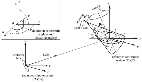
Figure 2.
Schematic diagram of the target and three coordinate systems.
Assume that the target rotates about a rotation axis ON in the reference coordinate system, and its azimuth and elevation angle in the above coordinates are αR and βR with the angular velocity of ω. According to Rodriguez’ Equation (7), the rotation matrix R(t) can be expressed as:
where D is the skew symmetric matrix:
We make an assumption that the initial azimuth and elevation angle of the object is α0 and β0 in the reference coordinate system. Therefore, the initial unit vector of the symmetric axis is:
Therefore, at time t, the unit vector of symmetric axis is represented as:
The angle δ (the angle between the symmetric axis of the object and LOS) can be computed as follows:
We can obtain the position of the object and sensor by the ground-based radar system. is the unit direction vector of the LOS. Combining the above formulas together, the variation condition of δ is achieved:
In the above formula, D is a function of αR and βR, is related to α0 and β0, and can be acquired from the radar system.
2.4. Infrared Signature Model Simulation
From above analysis of infrared radiation principle and signature model of the spatial target, the emitted radiation can be calculated by Equations (2), (4), and (13). Control variable methods are used to design several different precession parameters, and contrast experiments have been carried out on the infrared radiation of two types of targets [11,12]. Target 1 has a small precession angle, a long motion period, and a higher attitude stability, while Target 2 has a relatively large precession angle and a short motion period. Then the radiation power of the object received by the sensor is shown in Figure 3, on the basis of several parameters’ assumptions shown in Table 1 [13,14,15].
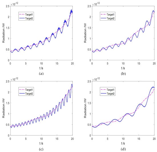
Figure 3.
Infrared radiation power curve of the cone object with coning micro-motion, (a–d) are the results of test 1, test 2, test 3, and test 4, respectively.

Table 1.
Table of parameter settings.
As depicted in Figure 3, the difference in infrared radiation characteristics of the two types of targets is mainly reflected in the difference of the attitude motion parameters in the case of the same shape, material, and initial temperature. When the precession angle is the same, the precession period has a greater influence on the infrared radiation. When the precession period is the same, the influence of the precession angle on the infrared radiation is relatively small. The regular attitude change of the target caused by precession conduces the periodic change of the projection area. This signal without noise is in the ideal situation.
We also studied the spatial targets of seven typical shapes, including flat-base cone, cone-cylinder, cylinder, and ball-base cone, equal curvature arc, non-equal curvature arc, and circular ring. Their 3D models were then built and the projected areas under different motion states simulated according to the above model, as shown in Table 2.
Table 2.
Table of projection area of several typical shapes.
The results show that the projection area sequence of the spatial target has the same fluctuation characteristics as the infrared radiation intensity sequence. The projection sequence fluctuation characteristics of different shape targets are differentiated, which can provide the basis and clues for the discrimination of spatial targets. For example, the projection area time series of the convex object has mirror symmetry inside a single period (i.e., within a single period, the first half period sequence and the second half period sequence are mirror symmetrical). This is because the projection area of the convex object in the nLOS direction is equal to the projection area in the −nLOS direction. Thus, when the target rotates γ around the fixed axis and rotates π − γ, the projection area is equal, and the mirror symmetry phenomenon occurs. Fragments do not have the symmetry of the projection area, so the projection area sequence usually does not have mirror symmetry. Moreover, under the same micro-motion parameters, the time-series fluctuation of the projection area of the debris is larger and the undulating characteristics are more obvious.
3. Shape Parameters Estimation Algorithm
The problem of unique shape identification and reconstruction based on projection area information has been widely concerned in the field of geometry. Alexandrov’s theorem states that the two origin symmetry convex shapes are identical if and only if both have the same projection area function [16].
Both the origin symmetrical convex and the semi-convex target have conditions for uniquely determining and reconstructing the shape. Targets with a semi-convex structure in the space target group, such as warheads and imitation baits, satisfy the conditions of unique shape determination and reconstruction.
3.1. Gaussian Image Representation
There are many ways to describe the shape of the target. However, most of the description methods, including the depth map, the normal stitch, etc., are affected by the target position and posture, and are not suitable for describing the shape of the spatial target. To this end, this section introduces a kind of shape description method suitable for attitude change, the Gaussian images method [17]. The basic idea is to establish the mapping relationship between the target surface and the unit Gaussian sphere according to the Gaussian curvature of the target surface.
If the Gaussian image representation method is used, the projection area will be greatly simplified as shown in the following Equation (15).
As shown in the Figure 4, assuming that the normal vector of the gray surface in the target surface is n, the vector n can be expressed by the azimuth angle α and the elevation angle β, that is, n(α, β) = [cosαcosβ, sinαcosβ, sinβ]. When the Gaussian image representation of the target is established, the gray surface is projected into the small area dαdβ of the unit sphere, and the area of the target gray surface is:
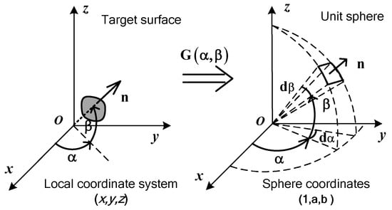
Figure 4.
Area conversion between the target surface and the Gaussian sphere.
The projection area calculation formula of the target becomes:
Equation (15) has a well-defined integration domain, and its shape information is mainly concentrated in the reciprocal G−1(α,β) of the Gaussian curvature, which makes the shape estimation problem more clear.
3.2. Shape Discrete Description and Estimation
The solution to G−1(α,β) is morbid because the integral operation is tight and its inverse operation is necessarily non-tight. That is to say, there is no way to accurately estimate G−1(α,β) without any constraint or prior information. Therefore, in the shape estimation, it is necessary to establish a discrete representation of G−1(α,β) under certain constraints, and transform Equation (15) into a discrete linear representation, i.e.:
where A is the projection area vector of the target, g⇔ G−1(α,β)dαdβ contains discrete variables describing the shape of the target, and matrix D is the cosine calculation [7,8].
When G−1(α,β) is discretely sampled, g is the area of the patch corresponding to the discrete points of G−1(α,β).
For the sake of clarity, taking the truncated column target as an example to describe. As shown in Figure 5, the target body has a two-ring distribution of G−1(α,β) in the Gaussian image representation and an isolated point. In this case, it is suitable to discretely sample G−1(α,β) into a series of discrete points (αj, βj), j = 1, ..., N, so that each discrete point (αj, βj) corresponding to a small patch whose normal vector is n(αj, βj) on the target surface, the original target shape is approximated as a convex polyhedron. As the number of points for discrete sampling of G−1(α,β) increases, the shape of the convex polyhedron is shown to be closer to the original shape [18,19]. This shape description method is often referred to as a convex polyhedral representation method [20].
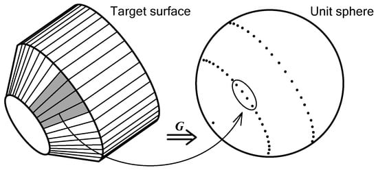
Figure 5.
Mapping of target discrete patches to a unit Gaussian sphere.
For an unknown target, the normal vector nj of the patch may be oriented in any direction of the three-dimensional space. In order to obtain all possible normal vectors npq(αp,βq), the warp and latitude of the 3-D sphere space are usually equally spaced (e.g., Δα, Δβ), where:
At this time, g in Equation (16) is all of the possible patch areas apq (p = 1, ..., N1; q = 1, ..., N2), and the projection area function of the target is also changed to:
When the projection area sequence data of the unknown target is obtained, the value of the unknown variable g can be estimated according to Equation (19). The unique convex polyhedron is reconstructed by g, thereby realizing the estimation and reconstruction of the convex target shape [6,21,22]. Since A = Dg is a linear model, the standard method for solving g is a least squares algorithm, and its optimization objective function can be expressed as:
The optimization objective function in Equation (20) is convex and has a unique minimum, and the conjugate descent gradient method is suitable in the optimization process.
3.3. Space Target Shape Estimation Experiment
The experiments estimate and reconstruct the target shape based on the simulated target projection area sequence. Since only the shape estimation problem is discussed, it is assumed that the micro-motion parameters of the target are known a priori. The purpose of the simulation experiment includes the following points: (1) test the performance of the estimation algorithm under different data noise levels; and (2) compare the shape estimation error caused by the deviation of the micro-motion parameters θ and ω, respectively.
Taking the tumbling cone target as the observation object, whose radius and cone height are 1.0 m and 5.6713 m, tumbling parameters are θ = 0.3π, α0 = 0.0π, β0 = 0.2π, ωt = 1.0π rad/s. In data acquisition, assume the observing time of infrared sensors is 6 s, and the scanning frequency is 20 Hz. In the parameter estimation, N1 and N2 are 36 and 19, respectively. The experiment was divided into three groups to investigate the effects of data noise, precession angle θ and precession angular velocity ωt on shape estimation performance.
Group 1: The impact of test data noise on shape estimation.
The signal-to-noise ratio (SNR) is used in the experiment to describe the noise level in the observed data. The signal-to-noise ratio is defined as:
where σs, σn are the standard deviations of the observed signal and the Gaussian noise signal, respectively. Tests are made for the data of different noise levels.
According to the estimation results in Table 3, the degree of restoration of the reconstructed shape to the original shape is increase as the noise decreases. The reconstruction result of the shape is relatively accurate as long as the data SNR is greater than 10 dB, and explains the error of the shape parameters’ estimation is relatively small. When the SNR achieves 30 dB, the reconstructed shape of the target in the experiment has become a standard cone and is almost restored to the original shape, and the validity of the shape parameters’ estimation has been proved.
Table 3.
Shape reconstruction results of different noise data.
Group 2: Test the effect of precession angle θ deviation on shape estimation.
In the evaluation of the application, it is very important to understand the error caused by the micro-motion parameters’ deviation for shape reconstruction. In the experiment, the true precession angle θ is set to 0.30π, and the signal-to-noise ratio of the observed data is 30 dB. The other parameters are the same as the previous set of experiments.
Table 4 shows the results of the experiments. It can be seen that the shape reconstruction error is relatively small when the θ deviation Δθ ∈ [−0.025π, 0.025π]. The reconstructed shape is similar to a cone to some extent. Although the specific experimental results are not representative of all error conditions, it can be explained that θ has relatively less influence on shape reconstruction.
Table 4.
Shape reconstruction result under roll angle deviation.
Group 3: Test the effect of angular velocity ωt on shape estimation.
The tumbling angular velocity ωt determines the fluctuation period of the observed data and is a sensitive parameter in the estimation. Even a small deviation probably causes a large error in the shape estimation. The true precession angular velocity ωt is 0.1π rad/s, and the observed data signal-to-noise ratio is 30 dB. Other parameters are unchanged.
Adjusting the tumbling angular velocity and recording the shape reconstruction results in Table 5. The results show that when the value of exceeds 0.01π rad/s (that is 1% deviation), the reconstructed target shape has great difference with the original shape. It can be seen that the angular velocity ωt has a relatively large influence on shape estimation and reconstruction.
Table 5.
Shape reconstruction results under angular velocity deviation.
4. Shape and Micro-Motion Parameters’ Joint Estimation
4.1. Problem Description
The estimation of the micro-motion parameters of the spatial target is relatively simple compared to the shape estimation. Since the number of micro-motion parameters is extremely small, the data requirements for the estimation do not exceed the data requirements of the shape estimation. Therefore, the joint estimation of the geometrical shape and the micro-motion parameters can be effectively realized as long as the necessary conditions and data requirements of the shape estimation are satisfied. The main difficulty in the joint estimation of shape and micro-motion parameters is that the objective function χ2 in Equation (20) is a non-convex function relative to the micro-motion variable θ, δ, ω, φ0, and there are multiple minimum value points in the value space of the variable. In the joint estimation, how to choose the appropriate optimization techniques and strategies to ensure the global optimal value of the objective function is the main problem to be solved in this section.
The micro-motion parameters of the precession target include: precession angle θ, observation angle δ, initial surface angle φ0 of the cone rotation axis, angle ψ0 between the projection of the cone rotation axis on xOy and Ox, and the spin and cone angular velocities ωs and ωc. In the target projection area sequence function Aproj(t), the micro-motion variables are included in the infrared sensor detecting line of sight direction vector n′LOS, and the line of sight vector n′LOS (θ, δ, φ0, Ψ0, ωs, ωc) can be expressed as:
where ψ(t) = ωst + ψ0, φ(t) = ωct + φ0 is the surface angle of conical axis.
In order to ensure a unique solution in the parameter estimation, usually the preset azimuth angle α or the elevation angle β is known, so that α is always equal to the azimuth angle of nLOS. The unknown micro-motion parameters are changed from θ, δ, φ0, ψ0, ωs, ωc to θ, β, φ0, ψ0, ωs, ωc, and there is a unique solution to the micro-motion parameter estimation problem [23].
In addition, since the target is axisymmetric, ωs does not affect the observed data, so let ψ(t) ≡ 0, then the equation becomes:
Equation (23) is also the n′LOS expression when the target is rolled. For axisymmetric targets, the estimated parameters are the same including θ, β, φ0, ω (ω is ωc or ωt), whether they are precessing or tumbling [24].
According to Equation (19), the function of the projection area of the spatial target is expressed as:
where apq (p = 1, ..., N1; q = 1, ..., N2) is the shape parameter for the space target. In the form of Equation (16), the target micro-motion parameter estimation problem is expressed as:
where is the observation data in the time period t1, ..., tL, is the shape parameter vector of the spatial target, and is the nonlinear function of the micro-motion parameters θ, β, ω, φ0.
4.2. Joint Estimation Algorithm and Experiment
Similar to the shape parameter estimation, the joint estimation also uses the least squares optimization algorithm, i.e.:
By analyzing the objective function of Equation (26), we know: (1) under the condition of known micro-motion parameters, the optimal estimation of the shape parameter g from function χ2 is convex; and 2) in the case of the known shape parameters, the estimation of micro-motion parameters θ, β, ω, φ0 from function χ2 is non-convex, and there are multiple local minima in the value space. Thus, the optimal non-convexity of the objective function χ2 in the joint estimation is mainly determined by θ, β, ω, φ0. Fortunately, θ, β, ω, φ0 have a clear value space, and χ2 is continually differentiable for θ, β, ω, φ0. Therefore, the grid search method is suitable for solving the joint optimal estimation problem. The value spaces of θ, β, ω, and φ0 are partitioned and searched one-by-one to obtain a global optimal solution.
First we can predefine β ∈ [0, 0.5π] to ensure that there is only a unique solution. Therefore, the range of values of θ, β, φ0 is redefined to θ ∈ [0, 0.5π], β ∈ [0, 0.5π], φ0 ∈ [0, 2π]. Only the value space of the angular velocity ω requires pre-processing or other measurement information to be determined.
4.2.1. Minimum Spacing Selection in the Grid Method
The idea of the grid method is to divide the value space of θ, β, ω, φ0 into blocks, and then search for the global optimal solution block by block. Thus, first it is necessary to determine the minimum spacing θΔ, βΔ, ωΔ, φ0Δ of the mesh segmentation to ensure that the number of local minima points is not more than 1 in each region. It is found that in the value space of the θ, β, φ0 parameters, the objective function χ2(θ,β,φ0) has only a finite number of local minimum values, and the minimum spacing is usually determined according to the experiment. However, there is a large number of local minimum values in the objective function χ2(ω) in value space of ω. We know that ω is the frequency parameter of the periodic sequence and the minimum value distribution and the minimum spacing value often have statistical laws to follow.
By statistically analyzing of the function χ2(ω) curve (assuming other parameters θ, β, φ0 are known), we found that it is reasonable to select half of the minimum interval P2/T as the division interval:
where ω is the true value of angular velocity.
In summary, the process of our estimation algorithm is shown in Algorithm 1.
| Algorithm 1 Diagram of our estimation. |
| Input: projection area of spatial target dataset, line of sight vector nLOS. |
| Output: estimation of micro-motion parameters , , , , and shape parameters . |
| Step 1 Initialization |
| (1) determine the range of values for ; (2) confirm the value space of θ, β, ω, φ, and divide the grid area and try to ensure that there is no more than one minimum value in each block; (3) randomly select the initial value of the variable in each block θ0, β0, ω0, φ00. |
| Step2 Search for a minimum value in a single grid to get , , , and the objective function value χ2. |
| Step 3 Select the minimum χ2 corresponding to , , , in all grid areas as the final output. |
4.2.2. Estimation Experiment
The simulation experiment explores the optimal estimation problem of joint parameters. The purpose is to determine the meshing distances θΔ, βΔ, φ0Δ of θ, β, φ0, and test the performance of the joint estimation of the shape and micro-motion parameters. The experiment is divided into three groups: the first group determines the meshing interval θΔ, βΔ, φ0Δ of the θ, β, φ0 parameters; the second group verifies the approximation law between Δω and the observation time T and the rotation period P in Equation (27) is accurate. Group 3 explores the performance of the algorithm for shape and micro-motion parameter estimation at different noise levels.
In the dataset acquisition, the infrared sensor scan frequency is 20 Hz, the observation time is T = 10 s, and the detection line of sight direction nLOS = [0.9511, 0, −0.3090]. The observed object is a tumbling cone target with a radius and cone height of 1.0 m and 5.6713 m, respectively. The precession parameters are θ = 0.3π, φ0 = 0.4π, αt = 0.0π, βt = 0.2π, ωt = 1.0π rad/s. In the experiment, the initial value is randomly selected and tested several times. When the random convergence rate reaches 90% or more, it is considered that the effective convergence condition is satisfied.
Group 1: Determine the meshing pitch θΔ, βΔ, φ0Δ of θ, β, φ0 parameters.
This group of experiments focuses on the division of the value space of θ, β, φ0, so we first limit the value of ω to [0.9375π, 1.0625π] rad/s, i.e., ωΔ = 0.1π rad/s, the condition satisfies the selection requirement of ωΔ when T = 8 s. As pointed out in the foregoing, θ, β, φ0 have a clearly finite value space, namely θ ∈ [0, 0.5π], β ∈ [0, 0.5π], φ0 ∈ [0, 2π], in determining the meshing pitch. It is usually obtained empirically.
In the experiment, the initial values of θ, β, and φ0 were randomly selected for 100 repeated tests, and the pitches were set to 0.5π, 0.25π, and 0.125π, respectively. At this time, the number of times to converge to the global minimum point χ2 ≤ 0.01 was 45, 96, and 100 times. Therefore, when the pitch is 0.25π or less, the optimization algorithm can achieve effective convergence. We also discovered that when the spacing is 0.25π, there are four times that θ, β, φ0 only converge to a local minimum χ2 ≈ 0.395, failing to converge to the global minimum. The reasons may be: (1) the gradient descent algorithm has no ability to cross the saddle point; or (2) the sampling rate is too low, and the amount of data information is slightly insufficient.
Group 2: Verify the approximation between ωΔ and the observation time T and the angular velocity true value ω.
The conclusion of Equation (27) indicates that it should be half of P/T. In order to verify the correctness of the conclusion, the experiment was tested for T = 6 s, 8 s, 10 s (P = 2 s). According to Equation (27), the division interval of the value range of ω should be 0.167π, 0.125π, 0.10π rad/s, and the grid division pitch of other parameters, such as θ, β, φ0, is 0.25π. After 100 repeated tests, 95, 96, and 94 times, respectively, converge to the global minimum, which proves the correctness of the conclusion in Equation (27). This conclusion is an important prerequisite for the joint estimation problem.
Group 3: Test the estimation error of shape and micro-motion parameters θ, β, ω, φ0 at different noise levels.
In the experiment, the signal-to-noise ratio (SNR) is used to describe the noise level in the observed data. The observation time is T = 10 s, and the division interval of the micro-motion parameters θ, β, ω, φ0 is determined according to the first group and the second group. The error of the estimation results of the micro-motion parameters Δθ, Δβ, Δφ0, Δω in the different noise levels are listed in Table 6.
Table 6.
Micro-motion parameter estimation results of different noise data.
According to the experimental results, when the data noise level is low, for example when the SNR > 10 dB, the optimization algorithm can converge to the global minimum, and the accuracy and reliability of the shape and micro-motion parameter estimation results are higher. The reconstructed shape has been restored to its original shape to a large extent, and demonstrates the validity of the joint estimation algorithm for shape parameter estimation. The errors of the estimated value of the micro-motion parameter are very small, as shown in the Table 6. The optimization algorithm is difficult to converge when the data noise is high, and the error of the estimation result is relatively large. The reason is that the details of the radiation intensity sequence of the target caused by micro-motion which makes it possible to be distinguished are easily masked by noise in a noisy environment. Under the same experimental conditions, when SNR > 10 dB, Liu [5] obtained micro-motion parameter estimation results of Δθ < 0.025π rad, Δβ < 0.002π rad, Δφ0 < 0.015π rad, and Δω < 0.01π rad/s. Compared with our method, we find that Liu’s method performs better in the estimation of parameter β, but the results of our methods in estimation of ω, θ, and φ0 are better than those of Liu.
5. Conclusions
This paper investigated the method of estimating the micro-motion and geometry parameters of spatial targets from the received infrared signatures. Firstly, based on the geometric and attitude motion analysis to construct the infrared feature model, we derive the mathematical formula of the space target projection region with micro-motion. Secondly, we used the least squares optimization algorithm to estimate the shape parameters of the spatial target with a Gaussian image representation to describe the discrete parameters of the shape. Finally, a joint estimation algorithm involving optimization techniques is proposed to solve the estimation problem of shape and micro-motion parameters. Aiming at the problem that the optimization objective function is a non-convex function, a solution to search the global optimal solution by the grid method is proposed to avoid the local minimum value. Simulation results show that the proposed method can guarantee the reliability of joint estimation of shape and micro-motion parameters.
However, the extraction of spatial target features in practical applications usually faces many difficulties. For example, in complex observation environments, received data by the detector may have insufficient observation conditions or high data noise, and the amount of data information cannot meet the data requirements of the parameter estimation. Target feature extraction methods under the condition of insufficient observation data will be studied in future research.
Author Contributions
D.W. wrote the manuscript and was responsible for the signal model design, parameter estimating algorithm design, and analysis. H.L., B.Z., J.L., and M.Z. assisted in the methodology development and signal model design and participated in the writing of the manuscript and its revision.
Funding
This work is supported by the Automatic Target Recognition Laboratory, National University of Defense Technology.
Conflicts of Interest
The authors declare no conflict of interest.
References
- Resch, C.L. Neural network for exo-atmospheric target discrimination. Proc. SPIE Int. Soc. Opt. Eng. 1998, 3371, 119–128. [Google Scholar]
- Zhu, D.; Shen, W.; Cai, G.; Ke, W. Numerical simulation and experimental study of factors influencing the optical characteristics of a spatial target. Appl. Therm. Eng. 2013, 50, 749–762. [Google Scholar] [CrossRef]
- Wang, H.; Zhang, W.; Wang, F. Infrared imaging characteristics of space-based targets based on bidirectional reflection distribution function. Infrared Phys. Technol. 2012, 55, 368–375. [Google Scholar] [CrossRef]
- Kaasalainen, M.; Torppa, J. Optimization methods for asteroid lightcurve inversion—I. shape determination. Icarus 2001, 153, 24–36. [Google Scholar] [CrossRef]
- Deng, Q.; Lu, H.; Xiao, S.; Wu, Y. Analysis of infrared signatures of exo-atmosphere micro-motion objects based on inertial parameters. Infrared Phys. Technol. 2018, 88, 32–40. [Google Scholar] [CrossRef]
- Liu, J.; Chen, S.; Lu, H.; Zhao, B. Ballistic targets micro-motion and geometrical shape parameters estimation from sparse decomposition representation of infrared signatures. Appl. Opt. 2017, 56, 1276–1285. [Google Scholar] [CrossRef]
- Bohren, C.; Clothiaux, E.; Johnson, N. Fundamentals of Atmospheric Radiation. Am. J. Phys. 2007, 75, 671. [Google Scholar]
- Zhang, W.; Li, K.; Jiang, W. Parameter estimation of radar targets with macro-motion and micro-motion based on circular correlation coefficients. IEEE Signal Process. Lett. 2015, 22, 633–637. [Google Scholar] [CrossRef]
- Calef, B.; Africano, J.; Birge, B.; Halla, D.; Kervin, P. Photometric signature inversion. Proc. SPIE 2016, 6307, 63070E. [Google Scholar]
- Qiu, C.; Zhang, Z.; Lu, H.; Zhang, K. Infrared modeling and imaging simulation of midcourse ballistic targets based on strap-down platform. J. Syst. Eng. Electron 2014, 25, 776–785. [Google Scholar] [CrossRef]
- Aumeunier, M.H.; Travere, J.M.; Reichle, R. Simulation of the infrared views of the upper port VIS/IR imaging system of ITER. IEEE Trans. Plasma Sci. 2014, 40, 753–760. [Google Scholar] [CrossRef]
- Liu, Z. Research on Techniques of Detection and Discrimination of Point Target in IR Image. Ph.D. Thesis, National University of Defense Technology, Changsha, China, 2005. [Google Scholar]
- Alam, M.S.; Bhuiyan, S.M. Trends in correlation-based pattern recognition and tracking in forward-looking infrared imagery. Sensors 2014, 14, 13437–13475. [Google Scholar] [CrossRef]
- Shi, L.; Cai, G.; Zhu, D. The simulation to infrared signatures of spacecraft. Astronautics 2009, 30, 229–234. [Google Scholar]
- Andrew, M.; Sessler, J.M.C.; Dietz, B. Countermeasures: A Technical Evaluation of the Operational Effectiveness of the Planned US National Missile Defense System. April 2000. Available online: http://www.ucsusa.org/sites/default/files/legacy/assets/documents/nwgs/cm_all.pdf (accessed on 16 October 2016).
- Gardner, R.J.; Milanfar, P. Reconstruction of convex bodies from brightness functions. Discret. Comput. Geom. 2003, 29, 279–303. [Google Scholar] [CrossRef][Green Version]
- Horn, B. Extended Gaussian Images. In Proceedings of the IEEE International Conference, New York, NY, USA, 8–11 October 1984; Volume 72, pp. 1671–1686. [Google Scholar]
- Linares, R.; Jah, M.; Crassidis, J.L.; Christopher, K.N. Space object shape characterization and tracking using light curve and angles data. J. Guid. Control. Dyn. 2014, 37, 13–26. [Google Scholar] [CrossRef]
- Lei, P.; Sun, J.; Wang, J.; Hong, W. Micromotion parameter estimation of free rigid targets based on radar micro-Doppler. IEEE Trans. Geosci. Remote Sens. 2012, 50, 3776–3786. [Google Scholar] [CrossRef]
- Holzinger, M.J.; Alfriend, K.T.; Wetterer, C.J.; Luu, K.K.; Sabol, C.; Hamada, K. Photometric attitude estimation for agile space objects with shape uncertainty. J. Guid. Control. Dyn. 2014, 37, 921–932. [Google Scholar] [CrossRef]
- Liu, J.; Li, Y.; Chen, S.; Lu, H.; Zhao, B. Micro-motion dynamics analysis of ballistic targets based on infrared detection. J. Syst. Eng. Electron. 2017, 28, 472–480. [Google Scholar]
- Liu, J.; Wu, Y.; Lu, H.; Zhao, B. Micromotion dynamics and geometrical shape parameters estimation of exoatmospheric infrared targets. Opt. Eng. 2016, 55, 113103. [Google Scholar] [CrossRef]
- Li, K.; Liu, Y.; Huo, K.; Jiang, W. Estimation of micro-motion parameters based on cyclostationary analysis. IET Signal Process. 2010, 4, 218–223. [Google Scholar] [CrossRef]
- Zhao, B.; Lu, H.; Chen, S. Convolutional neural networks for time series classification. J. Syst. Eng. Electron. 2017, 28, 169. [Google Scholar] [CrossRef]


© 2019 by the authors. Licensee MDPI, Basel, Switzerland. This article is an open access article distributed under the terms and conditions of the Creative Commons Attribution (CC BY) license (http://creativecommons.org/licenses/by/4.0/).