Adaptive Algorithm on Block-Compressive Sensing and Noisy Data Estimation


Abstract
:1. Introduction
2. Preliminaries
2.1. Compressive Sensing
2.2. Block-Compressive Sensing (BCS)
2.3. Problems of BCS
- Most existing research papers of BCS do not perform useful analysis on image partitioning and then segment according to the analysis result [21,22]. The common partitioning method (n = B × B) of BCS only considers reducing the computational complexity and storage space problem without considering the integrity of the algorithm and other potential effects, such as providing a better foundation for subsequent sampling and reconstructing by combining the structural features and the information entropy of the image.
- The basic sampling method used in BCS is to sample each sub-block uniformly according to the total sampling rate (TSR), while the adaptive sampling method selects different sampling rates according to the sampling feature of each sub-block [23]. Specifically, the detail block allocates a larger sampling rate, and the smooth block matches a smaller sampling rate, thereby improving the overall quality of the reconstructed image at the same TSR. But the crux is that the studies of criteria (feature) used to assign adaptive sampling rates are rarely seen in recent articles.
- Although there are many studies on the improvement of the BCS iterative construction algorithm [24], few articles focus on optimizing the performance of the algorithm from the aspect of iteration stop criterion in the image reconstruction process, especially in the noise background.
3. Problem Formulation and Important Factors
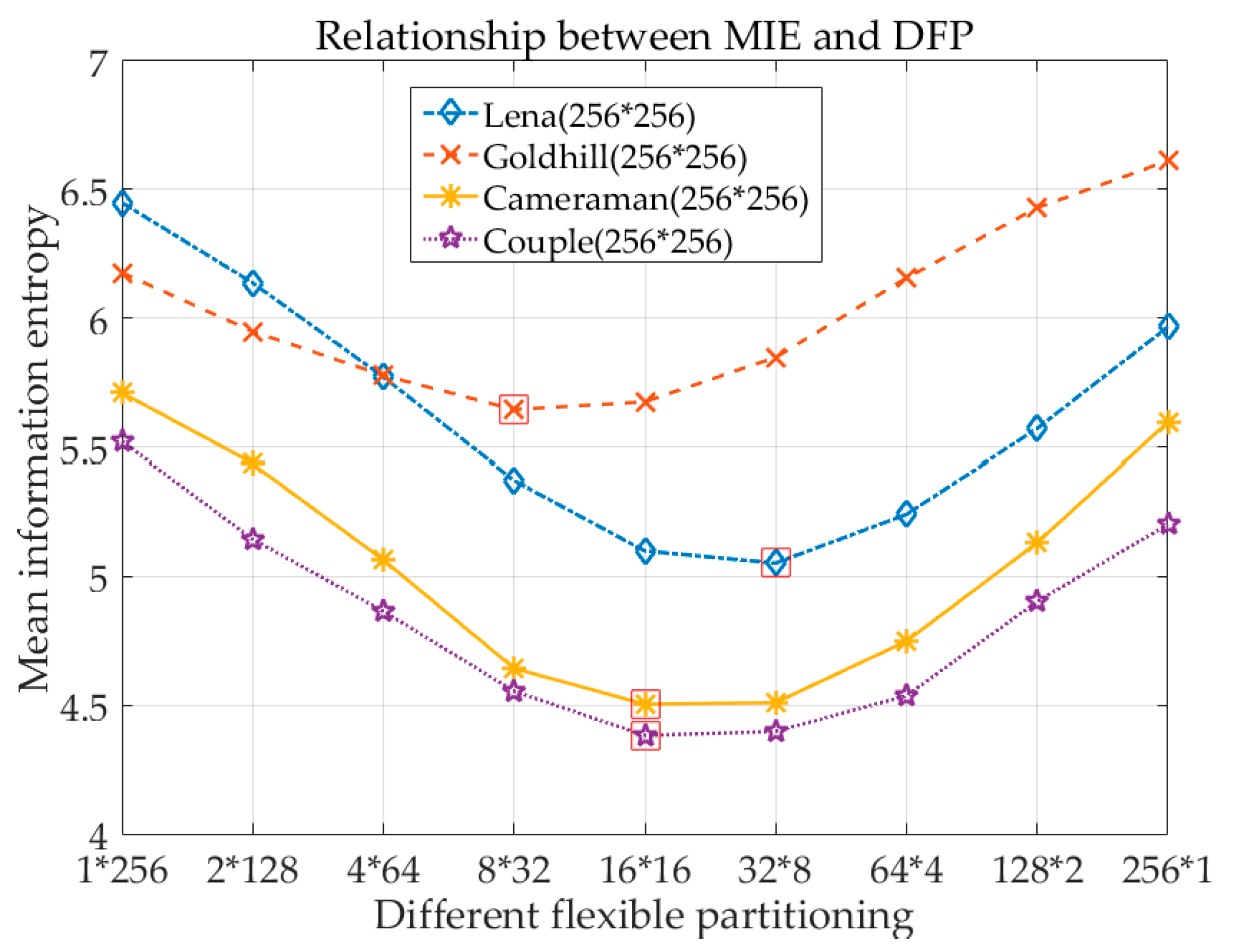
3.1. Flexible Partitioning by Mean Information Entropy (MIE) and Texture Structure (TS)
3.2. Adaptive Sampling with Variance and Local Salient Factor
3.3. Error Estimation and Iterative Stop Criterion in Reconstruction Process
3.3.1. Reconstruction Error Estimation in Noisy Background
3.3.2. Optimal Iterative Recovery of Image in Noisy Background
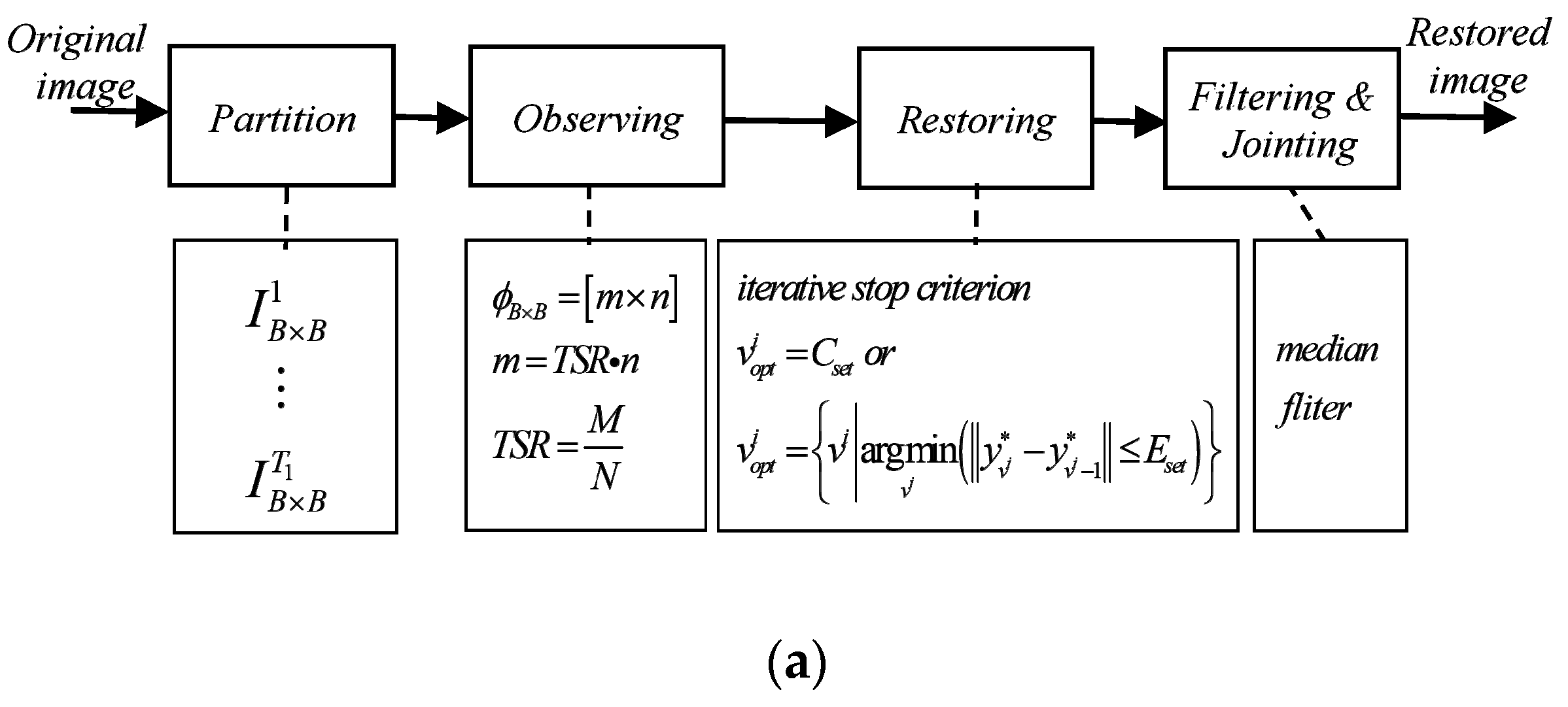
3.3.3. Application of Error Estimation on BCS
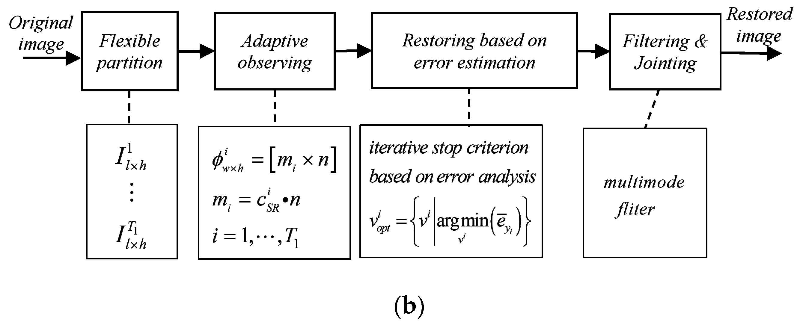
4. The Proposed Algorithm (FE-ABCS)
4.1. The Workflow and Pseudocode of FE-ABCS
- Flexible partitioning: using the weighted MIE as the block basis to reduce the average complexity of the sub-images from the pixel domain and the spatial domain;
- Adaptive sampling: adopting synthetic feature and step-less sampling to ensure a reasonable sample rate for each subgraph;
- Optimal number of iterations: using the error estimate method to ensure the minimum error output of the reconstructed image in the noisy background.
| FE-ABCS Algorithm based on OMP (Orthogonal Matching Pursuit) | |
| 1: Input: Original image I, total sampling rate TSR, sub-image dimension n (), sparse matrix , initialized measurement matrix 2: Initialization: ; ; // ; // step1: flexible partitioning (FP) 3: for j = 1,…,T2 do 4: ; ; 5: ; ; 6: ; // Weighted MIE--Base of FP 7: end for 8:; 9:; ; ; step2: adaptive sampling (AS) 10: for i = 1,…,T1 do 11: ; ; ; // synthetic feature (J)--Base of AS 12: end for 13: ; 14: ; // --AS ratio of sub-images ; 15: ; 16: ; 17: ; | step3: restoring based on error estimation 18:; // 19: ; 20: for i = 1,…,T1 do 21: ; //-- column vector of 22: ; // calculate optimal iterative of sub-images 23: for do 24: ; 25: ; 26: ; 27: end for 28: ; // --reconstructed sparse representation 29: ; // --reconstructed original signal 30: end for 31: ; // --reconstructed image without filter step4: multimode filtering (MF) 32: ; // 33: ; 34: 35: ; // 36: ; 37: ; 38: 39: // --reconstructed image with M |
4.2. Specific Parameter Setting of FE-ABCS
4.2.1. Setting of the Weighting Coefficient
4.2.2. Setting of the Adaptive Sampling Rate
- Initial value calculation of : get the initial value of the sampling factor by Equation (10).
- Judgment of through MSRF (): if the corresponding sampling rate factor of all image sub-blocks meets the minimum threshold requirement (), there is no need for modification, however, if it is not satisfied, modify it.
- Modifying of : if , then ; if , then use the following equation to modify the value:where, is the number of sub-images that can meet the requirement of the minimum threshold.
4.2.3. Setting of the Iteration Stop Condition
5. Experiments and Results Analysis
5.1. Experiment and Analysis without Noise
5.1.1. Performance Comparison of Various Algorithms
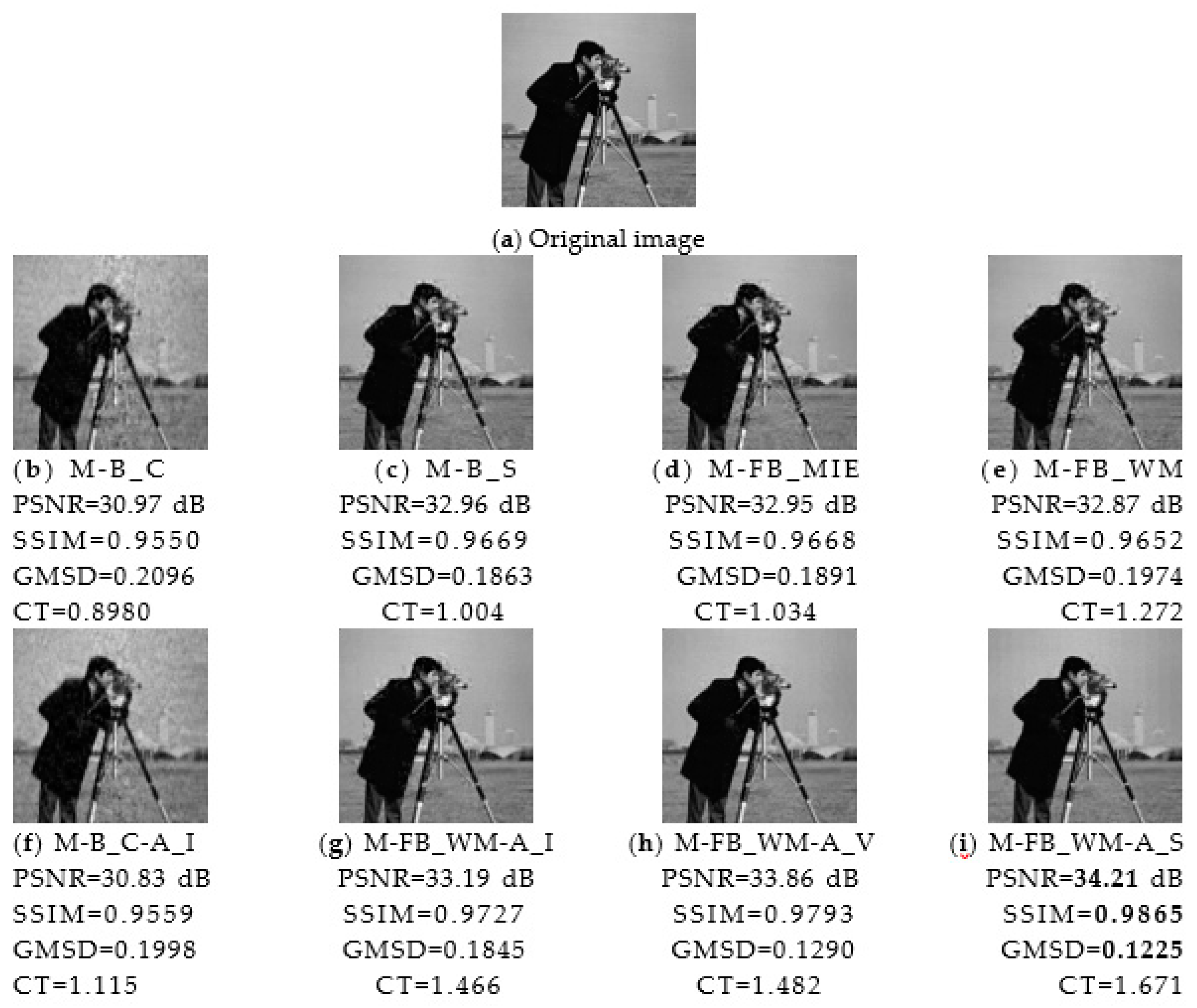
- Analysis of the performance indicators of the first four algorithms shows that for the BCS algorithm, BCS with a fixed column block is inferior to BCS with a fixed square block because square partitioning makes good use of the correlation of intra-block regions. MIE-based partitioning minimizes the average amount of information entropy of the sub-images. However, when the overall image has obvious texture characteristics, simply using MIE as the partitioning basis may not necessarily achieve a good effect, and the BCS algorithm based on weighted MIE combined with the overall texture feature can achieve better performance indicators.
- Comparing the adaptive BCS algorithms under different features in Table 1, variance has obvious superiority to IE among the single features, because the variance not only contains the dispersion of gray distribution but also the relative difference of the individual gray distribution of sub-images. In addition, the synthetic feature (combined local saliency) has a better effect than a single feature. The main reason for this is that the synthetic feature not only considers the overall difference of the subgraphs, but also the inner local-difference of the subgraphs.
- Combining experimental results of the eight BCS algorithms in Table 1 reveals that using adaptive sampling or flexible partitioning alone does not provide the best results, but the proposed algorithm combining the two steps will have a significant effect on both PSNR and SSIM.
5.1.2. Parametric Analysis of the Proposed Algorithm
5.2. Experiment and Analysis Under Noisy Conditions
5.2.1. Effect Analysis of Different Iteration Stop Conditions on Performance
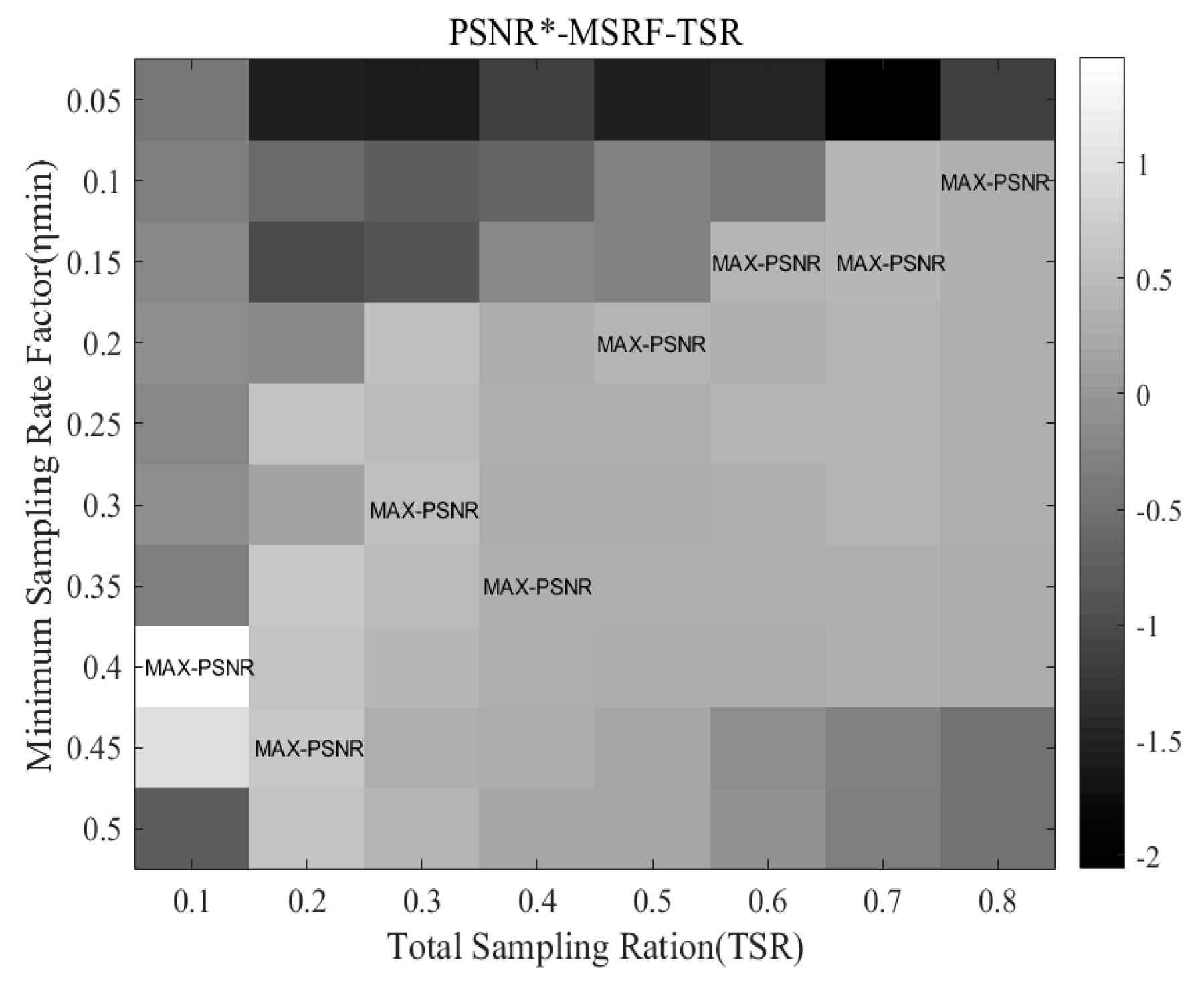
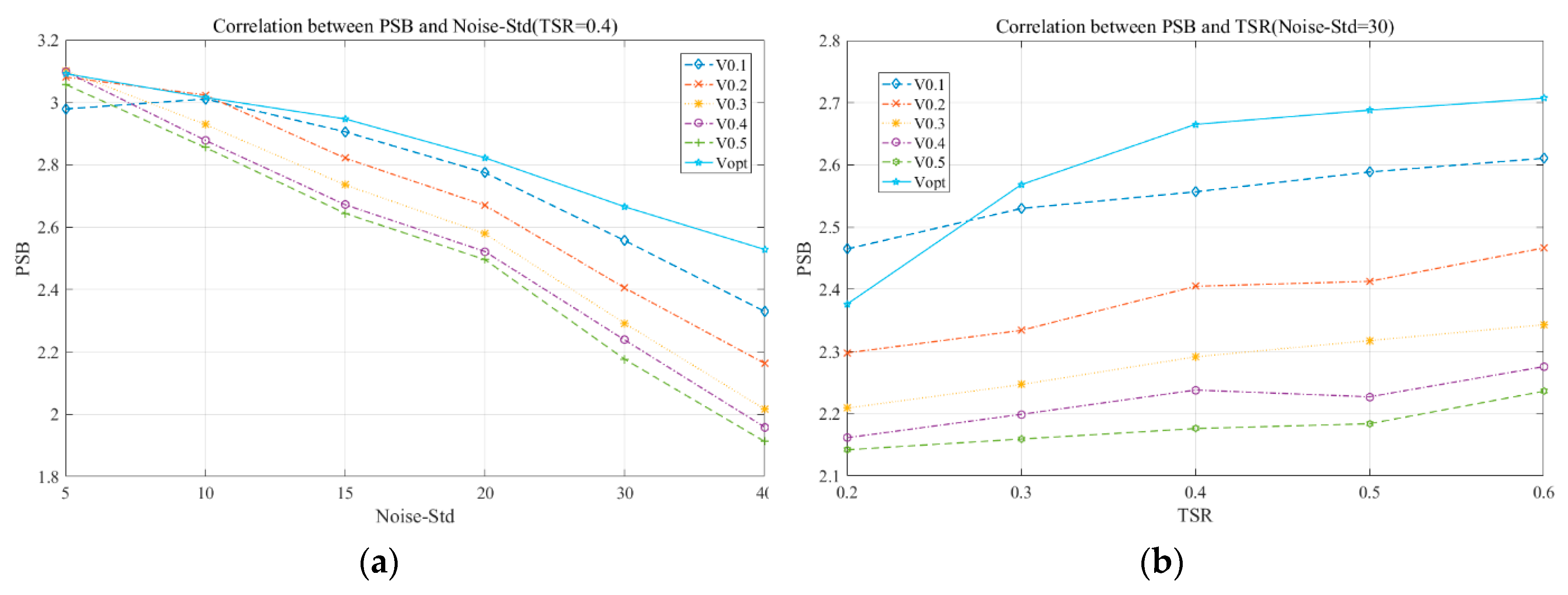
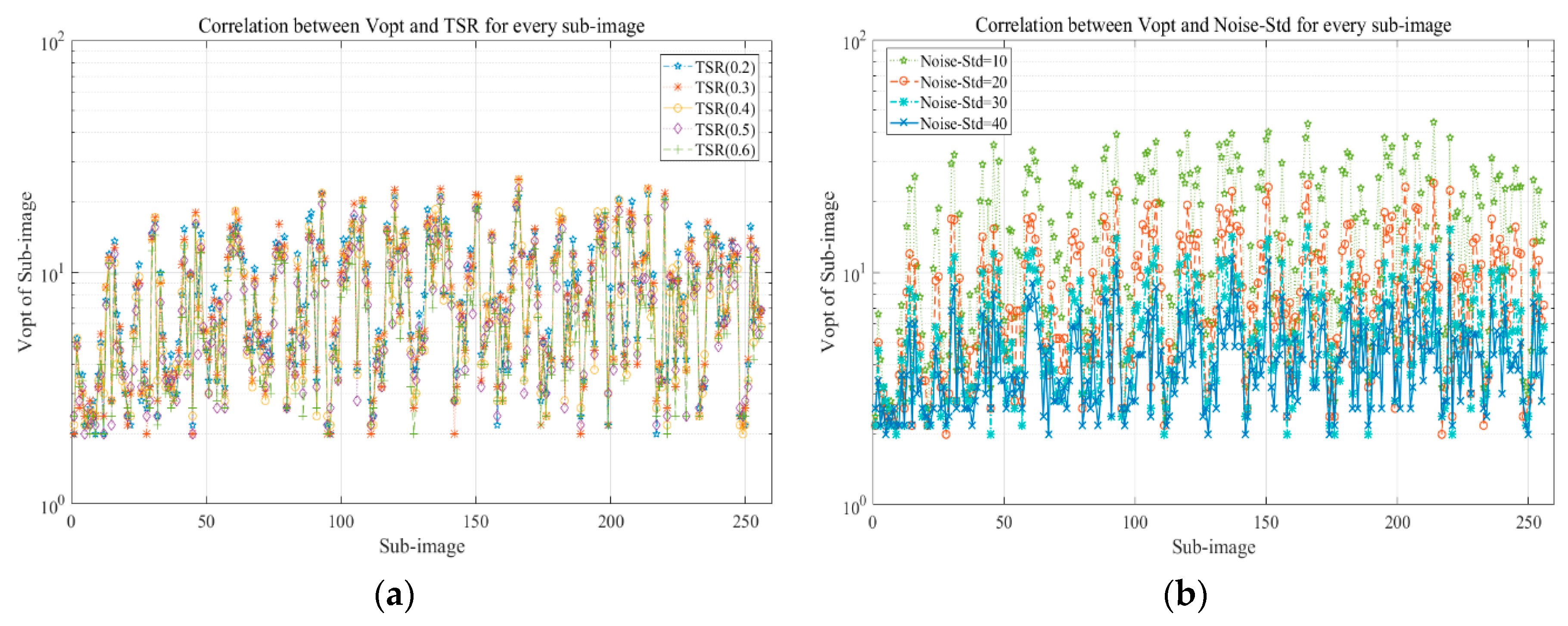
5.2.2. Impact of Noise-Std and TSR on
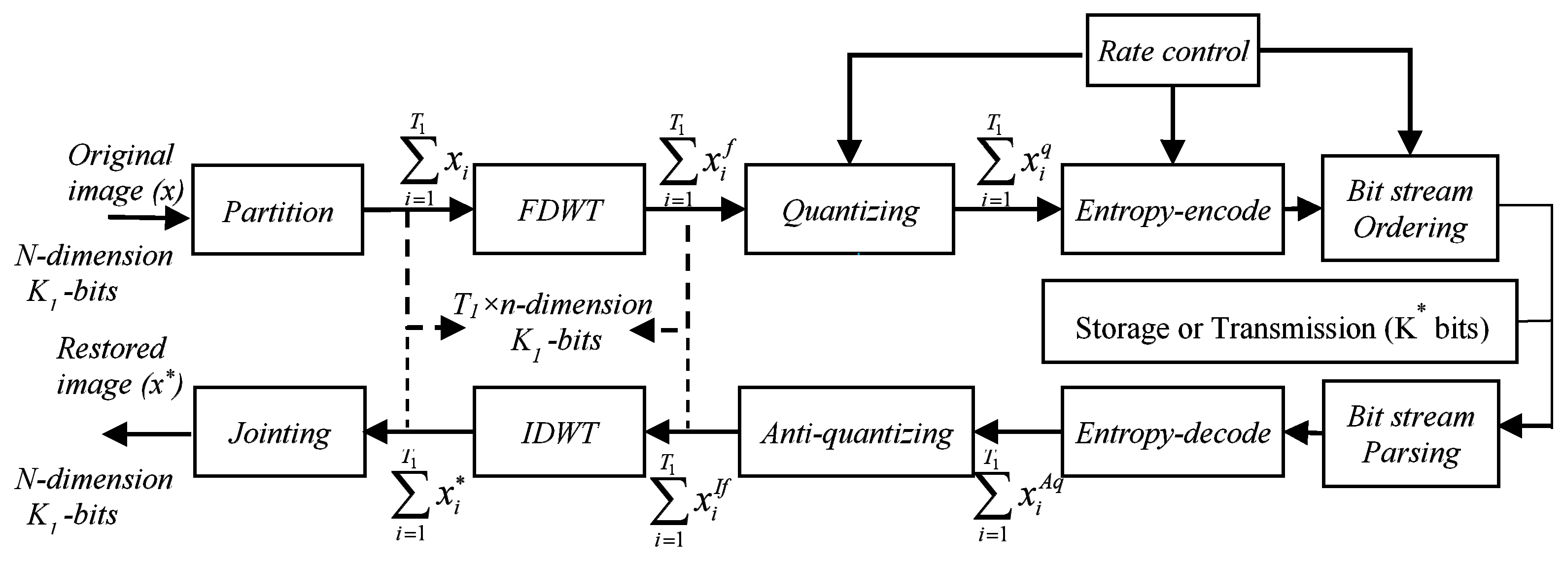
5.3. Application and Comparison Experiment of FE-ABCS Algorithm in Image Compression
5.3.1. Application of FE-ABCS Algorithm in Image Compression
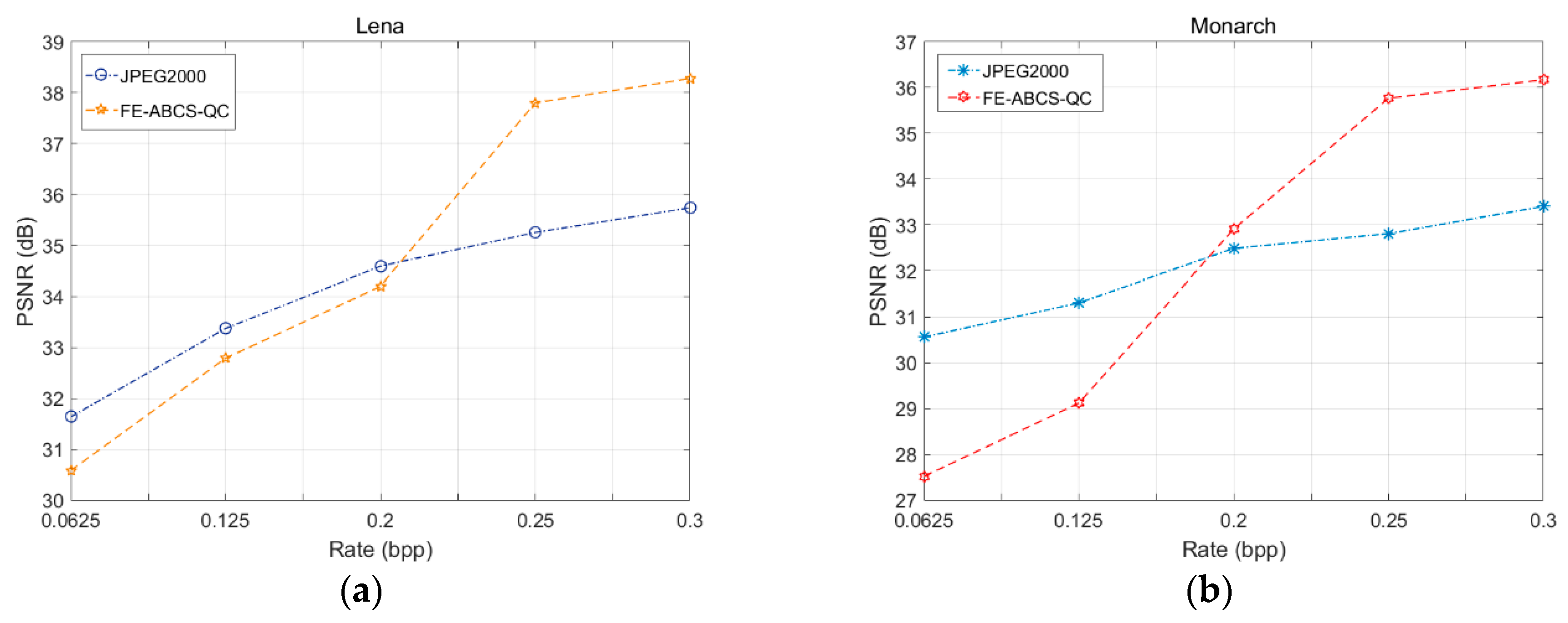
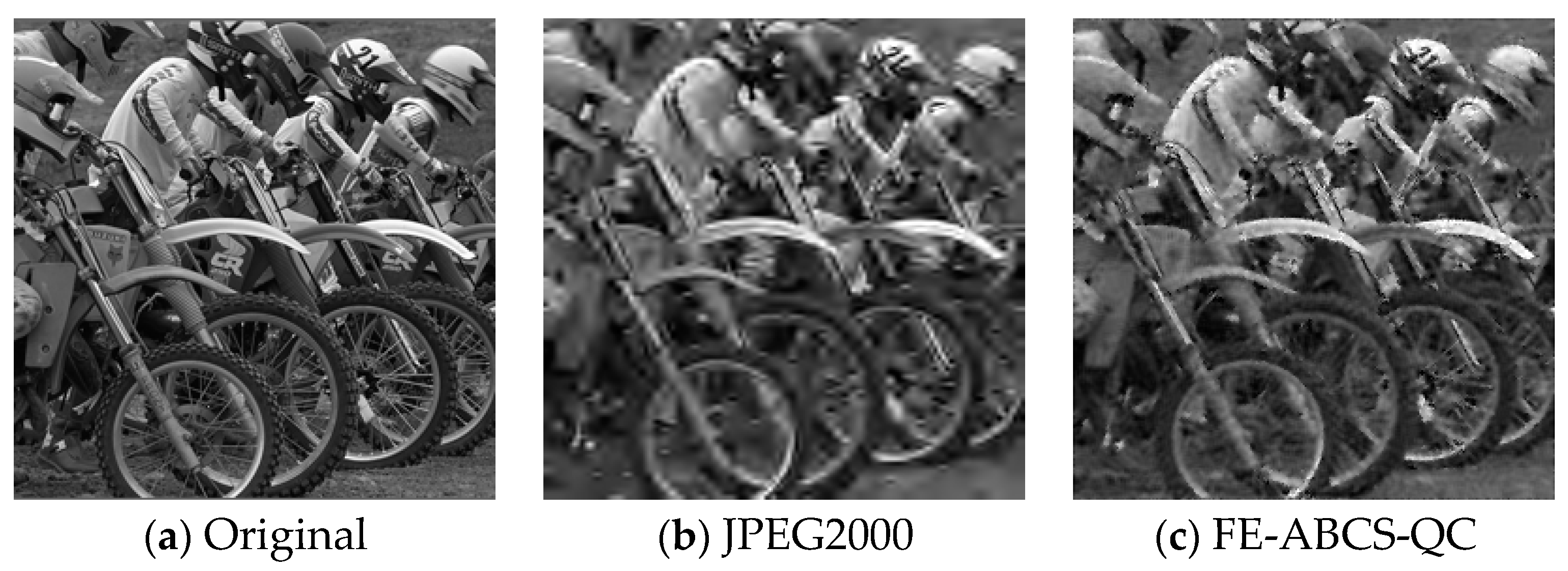
5.3.2. Comparison Experiment between the Proposed Algorithm and the JPEG2000 Algorithm
- Small Rate (bpp): the reason why the performance of the FE-ABCS-QC algorithm is worse than the JPEG2000 algorithm at this condition is that the small value of M which changes with Rate causes the observing process to fail to cover the overall information of the image.
- Medium or slightly larger Rate (bpp): the explanation for the phenomenon that the performance of the FE-ABCS-QC algorithm is better than the JPEG2000 algorithm in this situation is that the appropriate M can ensure the complete acquisition of image information and can also provide a certain image compression ratio to generate a better basis for quantization and encoding.
- Large Rate (bpp): this case of the FE-ABCS-QC algorithm is not considered because the algorithm belongs to the CS algorithm and requires M << N itself.
6. Conclusions
Author Contributions
Funding
Conflicts of Interest
References
- Donoho, D.L. Compressed sensing. IEEE Trans. Inf. Theory 2006, 52, 1289–1306. [Google Scholar] [CrossRef]
- Candès, E.J.; Wakin, M.B. An introduction to compressive sampling. IEEE Signal Process. Mag. 2008, 25, 21–30. [Google Scholar] [CrossRef]
- Shi, G.; Liu, D.; Gao, D. Advances in theory and application of compressed sensing. Acta Electron. Sin. 2009, 37, 1070–1081. [Google Scholar]
- Sun, Y.; Xiao, L.; Wei, Z. Representations of images by a multi-component Gabor perception dictionary. Acta Electron. Sin. 2008, 34, 1379–1387. [Google Scholar]
- Xu, J.; Zhang, Z. Self-adaptive image sparse representation algorithm based on clustering and its application. Acta Photonica Sin. 2011, 40, 316–320. [Google Scholar]
- Wang, G.; Niu, M.; Gao, J.; Fu, F. Deterministic constructions of compressed sensing matrices based on affine singular linear space over finite fields. IEICE Trans. Fundam. Electron. Commun. Comput. Sci. 2018, 101, 1957–1963. [Google Scholar] [CrossRef]
- Li, S.; Wei, D. A survey on compressive sensing. Acta Autom. Sin. 2009, 35, 1369–1377. [Google Scholar] [CrossRef]
- Palangi, H.; Ward, R.; Deng, L. Distributed compressive sensing: A deep learning approach. IEEE Trans. Signal Process. 2016, 64, 4504–4518. [Google Scholar] [CrossRef]
- Chen, C.; He, L.; Li, H.; Huang, J. Fast iteratively reweighted least squares algorithms for analysis-based sparse reconstruction. Med. Image Anal. 2018, 49, 141–152. [Google Scholar] [CrossRef]
- Gan, L. Block compressed sensing of natural images. In Proceedings of the 15th International Conference on Digital Signal Processing, Cardiff, UK, 1–4 July 2007; pp. 403–406. [Google Scholar]
- Unde, A.S.; Deepthi, P.P. Fast BCS-FOCUSS and DBCS-FOCUSS with augmented Lagrangian and minimum residual methods. J. Vis. Commun. Image Represent. 2018, 52, 92–100. [Google Scholar] [CrossRef]
- Kim, S.; Yun, U.; Jang, J.; Seo, G.; Kang, J.; Lee, H.N.; Lee, M. Reduced computational complexity orthogonal matching pursuit using a novel partitioned inversion technique for compressive sensing. Electronics 2018, 7, 206. [Google Scholar] [CrossRef]
- Qi, R.; Yang, D.; Zhang, Y.; Li, H. On recovery of block sparse signals via block generalized orthogonal matching pursuit. Signal Process. 2018, 153, 34–46. [Google Scholar] [CrossRef]
- Figueiredo, M.A.T.; Nowak, R.D.; Wright, S.J. Gradient projection for sparse reconstruction: Application to compressed sensing and other inverse problems. IEEE J. Sel. Areas Commun. 2007, 1, 586–597. [Google Scholar] [CrossRef]
- Lotfi, M.; Vidyasagar, M. A fast noniterative algorithm for compressive sensing using binary measurement matrices. IEEE Trans. Signal Process. 2018, 66, 4079–4089. [Google Scholar] [CrossRef]
- Yang, J.; Zhang, Y. Alternating direction algorithms for l1 problems in compressive sensing. SIAM J. Sci. Comput. 2011, 33, 250–278. [Google Scholar] [CrossRef]
- Yin, H.; Liu, Z.; Chai, Y.; Jiao, X. Survey of compressed sensing. Control Decis. 2013, 28, 1441–1445. [Google Scholar]
- Dinh, K.Q.; Jeon, B. Iterative weighted recovery for block-based compressive sensing of image/video at a low subrate. IEEE Trans. Circ. Syst. Video Technol. 2017, 27, 2294–2308. [Google Scholar] [CrossRef]
- Liu, L.; Xie, Z.; Yang, C. A novel iterative thresholding algorithm based on plug-and-play priors for compressive sampling. Future Internet 2017, 9, 24. [Google Scholar]
- Wang, Y.; Wang, J.; Xu, Z. Restricted p-isometry properties of nonconvex block-sparse compressed sensing. Signal Process. 2014, 104, 1188–1196. [Google Scholar] [CrossRef]
- Mahdi, S.; Tohid, Y.R.; Mohammad, A.T.; Amir, R.; Azam, K. Block sparse signal recovery in compressed sensing: Optimum active block selection and within-block sparsity order estimation. Circuits Syst. Signal Process. 2018, 37, 1649–1668. [Google Scholar]
- Wang, R.; Jiao, L.; Liu, F.; Yang, S. Block-based adaptive compressed sensing of image using texture information. Acta Electron. Sin. 2013, 41, 1506–1514. [Google Scholar]
- Amit, S.U.; Deepthi, P.P. Block compressive sensing: Individual and joint reconstruction of correlated images. J. Vis. Commun. Image Represent. 2017, 44, 187–197. [Google Scholar]
- Liu, Q.; Wei, Q.; Miao, X.J. Blocked image compression and reconstruction algorithm based on compressed sensing. Sci. Sin. 2014, 44, 1036–1047. [Google Scholar]
- Wang, H.L.; Wang, S.; Liu, W.Y. An overview of compressed sensing implementation and application. J. Detect. Control 2014, 36, 53–61. [Google Scholar]
- Xiao, D.; Xin, C.; Zhang, T.; Zhu, H.; Li, X. Saliency texture structure descriptor and its application in pedestrian detection. J. Softw. 2014, 25, 675–689. [Google Scholar]
- Haralick, R.M.; Shanmugam, K.; Dinstein, I.H. Texture features for image classification. IEEE Trans. Syst. Man Cybern. 1973, 3, 610–621. [Google Scholar] [CrossRef]
- Cao, Y.; Bai, S.; Cao, M. Image compression sampling based on adaptive block compressed sensing. J. Image Graph. 2016, 21, 416–424. [Google Scholar]
- Shen, J. Weber’s law and weberized TV restoration. Phys. D Nonlinear Phenom. 2003, 175, 241–251. [Google Scholar] [CrossRef]
- Li, R.; Cheng, Y.; Li, L.; Chang, L. An adaptive blocking compression sensing for image compression. J. Zhejiang Univ. Technol. 2018, 46, 392–395. [Google Scholar]
- Liu, H.; Wang, C.; Chen, Y. FBG spectral compression and reconstruction method based on segmented adaptive sampling compressed sensing. Chin. J. Lasers 2018, 45, 279–286. [Google Scholar]
- Li, R.; Gan, Z.; Zhu, X. Smoothed projected Landweber image compressed sensing reconstruction using hard thresholding based on principal components analysis. J. Image Graph. 2013, 18, 504–514. [Google Scholar]
- Gershgorin, S.; Donoho, D.L. Ueber die Abgrenzung der Eigenwerte einer Matrix. Izv. Akad. Nauk. SSSR Ser. Math. 1931, 1, 749–754. [Google Scholar]
- Beheshti, S.; Dahleh, M.A. Noisy data and impulse response estimation. IEEE Trans. Signal Process. 2010, 58, 510–521. [Google Scholar] [CrossRef]
- Beheshti, S.; Dahleh, M.A. A new information-theoretic approach to signal denoising and best basis selection. IEEE Trans. Signal Process. 2005, 53, 3613–3624. [Google Scholar] [CrossRef]
- Bottcher, A. Orthogonal symmetric Toeplitz matrices. Complex Anal. Oper. Theory 2008, 2, 285–298. [Google Scholar] [CrossRef]
- Duan, G.; Hu, W.; Wang, J. Research on the natural image super-resolution reconstruction algorithm based on compressive perception theory and deep learning model. Neurocomputing 2016, 208, 117–126. [Google Scholar] [CrossRef]


| Images | Algorithms | TSR = 0.2 | TSR = 0.3 | TSR = 0.4 | TSR = 0.5 | TSR = 0.6 |
|---|---|---|---|---|---|---|
| PSNR/SSIM | PSNR/SSIM | PSNR/SSIM | PSNR/SSIM | PSNR/SSIM | ||
| Lena | M-B_C | 29.0945/0.7684 | 29.8095/0.8720 | 30.6667/0.9281 | 31.8944/0.9572 | 32.9854/0.9719 |
| M-B_S | 31.1390/0.8866 | 31.7478/0.9227 | 32.4328/0.9480 | 33.2460/0.9651 | 34.2614/0.9763 | |
| M-FB_MIE | 30.7091/0.8613 | 31.2850/0.9115 | 32.0093/0.9413 | 32.9032/0.9600 | 33.8147/0.9737 | |
| M-FB_WM | 31.1636/0.8880 | 31.7524/0.9236 | 32.4623/0.9479 | 33.2906/0.9645 | 34.2691/0.9763 | |
| M-B_C-A_I | 29.1187/0.7838 | 29.8433/0.8803 | 30.8898/0.9305 | 32.0023/0.9577 | 33.2193/0.9732 | |
| M-FB_WM-A_I | 31.1763/0.8967 | 31.8872/0.9344 | 32.7542/0.9584 | 33.7353/0.9732 | 34.8647/0.9827 | |
| M-FB_WM-A_V | 31.2286/0.9087 | 32.0579/0.9433 | 33.0168/0.9643 | 34.1341/0.9775 | 35.4341/0.9856 | |
| M-FB_WM-A_S | 31.3609/0.9138 | 32.0943/0.9487 | 33.1958/0.9681 | 34.3334/0.9807 | 35.8423/0.9878 | |
| Goldhill | M-B_C | 28.4533/0.7747 | 28.9144/0.8718 | 29.3894/0.9080 | 29.7706/0.9315 | 30.2421/0.9495 |
| M-B_S | 29.5494/0.8785 | 29.9517/0.9089 | 30.3330/0.9341 | 30.8857/0.9514 | 31.4439/0.9640 | |
| M-FB_MIE | 29.7012/0.8882 | 29.9811/0.9154 | 30.4465/0.9364 | 30.9347/0.9516 | 31.5153/0.9642 | |
| M-FB_WM | 29.7029/0.8867 | 30.0277/0.9151 | 30.4827/0.9361 | 30.9555/0.9516 | 31.5333/0.9649 | |
| M-B_C-A_I | 28.4436/0.7809 | 28.8691/0.8693 | 29.3048/0.9089 | 29.7046/0.9321 | 30.2355/0.9499 | |
| M-FB_WM-A_I | 29.6708/0.8918 | 30.0833/0.9215 | 30.5120/0.9424 | 31.0667/0.9574 | 31.6899/0.9697 | |
| M-FB_WM-A_V | 29.5370/0.8957 | 30.0891/0.9253 | 30.5379/0.9456 | 31.0922/0.9607 | 31.8011/0.9724 | |
| M-FB_WM-A_S | 29.7786/0.8975 | 30.1482/0.9272 | 30.5689/0.9472 | 31.1310/0.9622 | 31.8379/0.9736 | |
| Cameraman | M-B_C | 28.5347/0.7787 | 29.0078/0.8559 | 29.3971/0.9051 | 29.9417/0.9379 | 30.6612/0.9592 |
| M-B_S | 31.1796/0.8763 | 31.4929/0.9121 | 31.9203/0.9391 | 32.3009/0.9581 | 32.7879/0.9704 | |
| M-FB_MIE | 31.1487/0.8782 | 31.5067/0.9123 | 31.8644/0.9403 | 32.3170/0.9577 | 32.7946/0.9703 | |
| M-FB_WM | 31.2118/0.8675 | 31.4645/0.9072 | 31.8130/0.9365 | 32.2050/0.9559 | 32.6811/0.9686 | |
| M-B_C-A_I | 28.5669/0.7852 | 28.8807/0.8612 | 29.3928/0.9164 | 29.9924/0.9461 | 30.6130/0.9639 | |
| M-FB_WM-A_I | 31.2554/0.8901 | 31.5975/0.9296 | 32.0955/0.9533 | 32.6859/0.9701 | 33.4007/0.9802 | |
| M-FB_WM-A_V | 31.2869/0.9085 | 31.8762/0.9550 | 32.5052/0.9746 | 33.3531/0.9848 | 34.4449/0.9904 | |
| M-FB_WM-A_S | 31.3916/0.9287 | 31.9731/0.9621 | 32.6508/0.9790 | 33.6779/0.9877 | 34.8958/0.9918 | |
| Couple | M-B_C | 28.6592/0.7582 | 29.0162/0.8557 | 29.5471/0.9109 | 30.2260/0.9440 | 30.9136/0.9640 |
| M-B_S | 30.1529/0.8912 | 30.6910/0.9289 | 31.2853/0.9541 | 31.9693/0.9695 | 32.7464/0.9796 | |
| M-FB_MIE | 30.1920/0.8895 | 30.7257/0.9282 | 31.2948/0.9531 | 31.9509/0.9692 | 32.7424/0.9794 | |
| M-FB_WM | 30.1357/0.8917 | 30.6890/0.9259 | 31.3185/0.9539 | 31.9520/0.9691 | 32.7622/0.9793 | |
| M-B_C-A_I | 28.5694/0.7428 | 29.0442/0.8589 | 29.5828/0.9088 | 30.2127/0.9444 | 30.9839/0.9642 | |
| M-FB_WM-A_I | 30.2105/0.9027 | 30.7783/0.9413 | 31.4680/0.9630 | 32.3143/0.9759 | 33.2604/0.9840 | |
| M-FB_WM-A_V | 30.1896/0.9099 | 30.8541/0.9454 | 31.4990/0.9670 | 32.3769/0.9792 | 33.3260/0.9864 | |
| M-FB_WM-A_S | 30.3340/0.9117 | 30.9047/0.9475 | 31.5496/0.9686 | 32.3788/0.9798 | 33.3561/0.9869 |
| Restoring Method | Algorithms | TSR = 0.4 | TSR = 0.6 | ||||||
|---|---|---|---|---|---|---|---|---|---|
| PSNR | SSIM | GMSD | CT | PSNR | SSIM | GMSD | CT | ||
| IRLS | R-B_C | 32.38 | 0.9361 | 0.1943 | 5.729 | 33.42 | 0.9790 | 0.1348 | 13.97 |
| R-B_S | 32.67 | 0.9634 | 0.1468 | 5.928 | 35.08 | 0.9843 | 0.0987 | 14.94 | |
| R-FB_MIE | 32.14 | 0.9593 | 0.1658 | 5.986 | 34.44 | 0.9825 | 0.1094 | 13.79 | |
| R-FB_WM | 32.46 | 0.9631 | 0.1441 | 6.071 | 34.80 | 0.9841 | 0.0992 | 14.25 | |
| R-B_C-A_I | 30.55 | 0.9460 | 0.1882 | 6.011 | 34.08 | 0.9825 | 0.1238 | 14.46 | |
| R-FB_WM-A_I | 33.05 | 0.9714 | 0.1346 | 6.507 | 36.01 | 0.9894 | 0.0863 | 14.98 | |
| R-FB_WM-A_V | 33.25 | 0.9751 | 0.1216 | 6.994 | 36.71 | 0.9914 | 0.0691 | 17.34 | |
| R-FB_WM-A_S | 33.59 | 0.9787 | 0.1188 | 7.456 | 37.23 | 0.9927 | 0.0661 | 19.38 | |
| BP | P-B_C | 30.56 | 0.9380 | 0.1984 | 33.47 | 33.35 | 0.9787 | 0.1378 | 69.67 |
| P-B_S | 32.72 | 0.9638 | 0.1484 | 34.22 | 34.61 | 0.9823 | 0.1072 | 71.00 | |
| P-FB_MIE | 32.00 | 0.9531 | 0.1627 | 34.04 | 34.14 | 0.9810 | 0.1149 | 68.78 | |
| P-FB_WM | 32.82 | 0.9635 | 0.1512 | 35.08 | 34.57 | 0.9832 | 0.1070 | 69.48 | |
| P-B_C-A_I | 30.72 | 0.9428 | 0.1973 | 33.84 | 33.57 | 0.9795 | 0.1335 | 70.27 | |
| P-FB_WM-A_I | 33.01 | 0.9705 | 0.1442 | 35.63 | 35.70 | 0.9884 | 0.0888 | 70.73 | |
| P-FB_WM-A_V | 33.32 | 0.9750 | 0.1277 | 36.98 | 36.37 | 0.9909 | 0.0742 | 72.59 | |
| P-FB_WM-A_S | 33.49 | 0.9773 | 0.1210 | 37.85 | 37.45 | 0.9932 | 0.0662 | 74.41 | |
| Sparsity | |||||||
|---|---|---|---|---|---|---|---|
| Noise-std | PSNR and SSIM and GMSD and BEI and CT | ||||||
| 5 | 32.95 | 32.71 | 32.39 | 32.12 | 31.96 | 32.48 | |
| 0.961 | 0.965 | 0.961 | 0.957 | 0.955 | 0.960 | ||
| 0.165 | 0.160 | 0.169 | 0.173 | 0.178 | 0.171 | ||
| 10.63 | 10.25 | 10.04 | 9.92 | 9.98 | 10.09 | ||
| 0.741 | 0.949 | 1.166 | 1.567 | 1.911 | 1.481 | ||
| 10 | 32.40 | 31.81 | 31.30 | 31.07 | 30.92 | 32.23 | |
| 0.957 | 0.955 | 0.949 | 0.941 | 0.937 | 0.956 | ||
| 0.169 | 0.179 | 0.190 | 0.194 | 0.200 | 0.177 | ||
| 10.29 | 10.04 | 10.14 | 10.15 | 10.20 | 10.21 | ||
| 0.741 | 0.922 | 1.233 | 1.637 | 1.961 | 0.926 | ||
| 15 | 31.63 | 30.87 | 30.46 | 30.27 | 30.12 | 31.81 | |
| 0.948 | 0.937 | 0.926 | 0.917 | 0.912 | 0.949 | ||
| 0.180 | 0.202 | 0.213 | 0.220 | 0.223 | 0.185 | ||
| 10.32 | 10.25 | 10.32 | 10.38 | 10.39 | 10.25 | ||
| 0.727 | 0.933 | 1.154 | 1.550 | 2.063 | 0.798 | ||
| 20 | 30.97 | 30.08 | 29.83 | 29.66 | 29.61 | 31.48 | |
| 0.936 | 0.916 | 0.898 | 0.887 | 0.879 | 0.941 | ||
| 0.197 | 0.219 | 0.236 | 0.244 | 0.247 | 0.191 | ||
| 10.45 | 10.34 | 10.39 | 10.43 | 10.43 | 10.50 | ||
| 0.720 | 0.914 | 1.203 | 1.476 | 2.348 | 0.739 | ||
| 30 | 30.03 | 29.34 | 29.04 | 28.94 | 28.89 | 30.75 | |
| 0.901 | 0.862 | 0.832 | 0.816 | 0.803 | 0.920 | ||
| 0.227 | 0.257 | 0.266 | 0.272 | 0.275 | 0.204 | ||
| 10.59 | 10.52 | 10.54 | 10.55 | 10.67 | 10.62 | ||
| 0.901 | 0.947 | 1.237 | 1.500 | 1.996 | 0.690 | ||
| 40 | 29.38 | 28.77 | 28.57 | 28.50 | 28.45 | 30.14 | |
| 0.856 | 0.795 | 0.756 | 0.734 | 0.717 | 0.899 | ||
| 0.252 | 0.277 | 0.286 | 0.290 | 0.291 | 0.221 | ||
| 10.79 | 10.57 | 10.71 | 10.68 | 10.67 | 10.72 | ||
| 0.736 | 0.791 | 1.169 | 1.534 | 2.047 | 0.678 | ||
| Images | Lena | Baboon | Flowers | Oriental Gate | Index | |
|---|---|---|---|---|---|---|
| Stop Condition | ||||||
| γ = 300 | 32.17 | 29.84 | 31.40 | 33.05 | PSNR | |
| 0.9562 | 0.8703 | 0.9744 | 0.9698 | SSIM | ||
| 0.1661 | 0.2095 | 0.1812 | 0.1636 | GMSD | ||
| 10.16 | 10.72 | 9.866 | 8.845 | BEI | ||
| 0.8310 | 0.855 0 | 0.844 0 | 1.050 | CT | ||
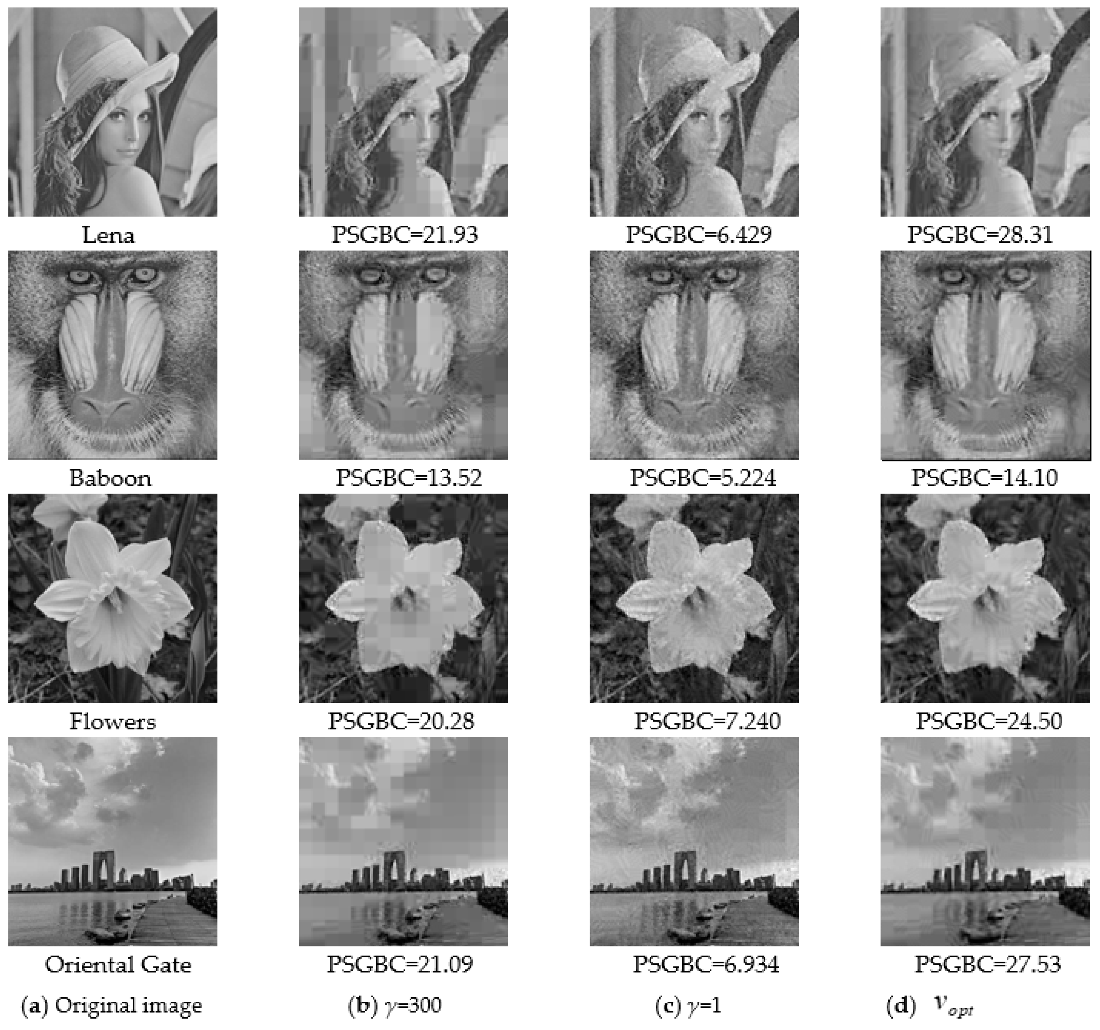
| 21.93 | 13.52 | 20.28 | 21.09 | PSGBC | ||
| γ =1 | 31.99 | 29.75 | 31.50 | 32.66 | PSNR | |
| 0.9574 | 0.8731 | 0.9768 | 0.9693 | SSIM | ||
| 0.1638 | 0.1738 | 0.1571 | 0.1459 | GMSD | ||
| 10.01 | 10.58 | 9.583 | 8.745 | BEI | ||
| 2.905 | 2.704 | 2.823 | 3.578 | CT | ||
| 6.429 | 5.224 | 7.240 | 6.934 | PSGBC | ||
| 32.75 | 30.03 | 31.78 | 33.15 | PSNR | ||
| 0.9603 | 0.8729 | 0.9771 | 0.9637 | SSIM | ||
| 0.1471 | 0.1956 | 0.1538 | 0.1471 | GMSD | ||
| 9.898 | 10.68 | 9.693 | 9.025 | BEI | ||
| 0.7630 | 0.8900 | 0.8500 | 0.8740 | CT | ||
| 28.31 | 14.10 | 24.50 | 27.53 | PSGBC | ||
| Method | JPEG2000 (PSNR/SSIM/GMSD) | FE-ABCS-QC (PSNR/SSIM/GMSD) | ∆P/∆S/∆G | |
|---|---|---|---|---|
| Test Image | ||||
| Lena | bpp = 0.0625 | 31.64/0.9387/0.1842 | 30.58/0.7341/0.2478 | −1.06/−0.2046/0.0636 |
| bpp = 0.125 | 33.38/0.9697/0.1399 | 32.79/0.9413/0.1702 | −0.59/−0.0284/0.0303 | |
| bpp = 0.2 | 34.59/0.9807/0.1161 | 34.20/0.9710/0.1339 | −0.39/−0.0097/0.0178 | |
| bpp = 0.25 | 35.25/0.9850/0.0996 | 37.80/0.9932/0.0612 | 2.55/0.0082/−0.0384 | |
| bpp = 0.3 | 35.73/0.9875/0.0917 | 38.28/0.9941/0.0554 | 2.55/0.0066/−0.0363 | |
| Monarch | bpp = 0.0625 | 30.56/0.8184/0.2335 | 27.52/0.3615/0.2726 | −3.04/−0.4569/0.0391 |
| bpp = 0.125 | 31.31/0.9074/0.1881 | 29.12/0.6388/0.2568 | −2.19/−0.2686/0.0687 | |
| bpp = 0.2 | 32.49/0.9466/0.1554 | 32.91/0.9473/0.1507 | 0.42/0.0007/−0.0047 | |
| bpp = 0.25 | 32.81/0.9572/0.1476 | 35.77/0.9886/0.0682 | 2.96/0.0314/−0.0794 | |
| bpp = 0.3 | 33.40/0.9679/0.1305 | 36.17/0.9896/0.0664 | 2.77/0.0217/−0.0641 |
© 2019 by the authors. Licensee MDPI, Basel, Switzerland. This article is an open access article distributed under the terms and conditions of the Creative Commons Attribution (CC BY) license (http://creativecommons.org/licenses/by/4.0/).
Share and Cite
Zhu, Y.; Liu, W.; Shen, Q. Adaptive Algorithm on Block-Compressive Sensing and Noisy Data Estimation. Electronics 2019, 8, 753. https://doi.org/10.3390/electronics8070753
Zhu Y, Liu W, Shen Q. Adaptive Algorithm on Block-Compressive Sensing and Noisy Data Estimation. Electronics. 2019; 8(7):753. https://doi.org/10.3390/electronics8070753
Chicago/Turabian StyleZhu, Yongjun, Wenbo Liu, and Qian Shen. 2019. "Adaptive Algorithm on Block-Compressive Sensing and Noisy Data Estimation" Electronics 8, no. 7: 753. https://doi.org/10.3390/electronics8070753
APA StyleZhu, Y., Liu, W., & Shen, Q. (2019). Adaptive Algorithm on Block-Compressive Sensing and Noisy Data Estimation. Electronics, 8(7), 753. https://doi.org/10.3390/electronics8070753