1. Introduction
Remarkable expansions in wireless communication systems (WCS) have been witnessed in the past few decades, including applications in indoor environments connected with personal communication and local area networks. The successful analysis, design, and the deployment of WCS requires a vast knowledge of propagation channel modeling. Background study shows that radio wave propagation prediction for various scenarios has become an active research topic [
1,
2,
3]. Accurate and faster propagation channel categorization depends mainly on the number of receivers, types of transmitter, and the propagation environment [
4]. It is also challenging to optimize the actual position of the transmitter (Tx) by measurement to ensure acceptable system performance. Therefore, radio-propagation using a simulation tool for the indoor environment based on RSSI and PL has become a significant research tool [
5].
Weather conditions—such as floods, rains, clouds, or snowfall—have no effect on the indoor radio propagation; however, it can be influenced by the interior walls, furniture, doors, windows, and other household objects. These influences need to be considered for better indoor radio wave propagation modeling. Therefore, the indoor scenario has these objects, with Tx waves reaching the receiver (Rx) through multipath channels [
6].
Although practical measurement enables actual assessment of onsite performance, it requires a sizable amount of resources and effort. On the other hand, software simulation tools are easy to use and are an inexpensive way to obtain accurate results [
7]. Nowadays, many researchers recommend the use of the RT technique for radio propagation prediction modeling [
8].
Based on the fundamental geometric optics (GO) theory and uniform theory of diffraction (UTD) principles, RT is extensively used in radio wave modeling, and is widely used in indoor WCS [
9]. The RT full cycle has three steps: ray launching (RL), ray path sensing, and ray capturing by receivers [
10]. The RL is the method of propagating straight rays in all directions in space. Normally, the rays are launched from the source of a Tx to the destination Rx by following the principle of GO and UTD. The complete ray path is traced, bearing the additional propagation features of transmission, reflection, and diffraction [
11]. At the end, in the ray capturing phase, the ray is estimated to have undergone an intersection with Rx or not, with a sphere area.
Reflection, refraction, and diffraction phenomena of RT require highly-configured computer resources applied to radio wave propagation prediction by RT. Several numerical and RT techniques, such as SBRT, the predetermined integration technique [
12], the prearranged element technique [
13], the finite differences time domain (FDTD) [
14,
15], and the combined ray tracing and FDTD hybrid method [
16] are used to improve the accuracy and reduce the computational time of the radio wave propagation prediction. Heuristic approaches perform well in simple environments at lower frequencies. In [
17], the mentioned exposure optimization for wireless networks uses heuristic approaches at 2.4–2.6 GHz. However, to support 5G potentials, frequencies in complex environments still need to consider the limitations of heuristic approaches. In [
18], the RT technique for radio propagation prediction used neural networks at 2.4 GHz, with ray launching horizontal and vertical angular resolution (π/360), by considering a maximum of seven number of reflections. Hence, an omnidirectional base station needs to handle
number of rays. In complex indoor environments with numerous obstacles to handle, more rays and a lot of time are needed. For higher frequency modeling, environmental effect on signal strength is likely, and so accurate results using a lower number of rays is considered a boon. Actually, there is no technique which completely satisfies the PL, RSSI, and the optimum number of rays launched for accurate propagation prediction, because of the trade-off correlation that exists among them. Among the various existing methods, the SBRT method is one of the most popular, and is extensively used in radio propagation channel characterization [
19].
However, when many potential Rx and Tx are positioned in a complex environment, conventional methods require a large amount of computational time and possess coverage limitations [
20,
21]. Conventional 3-D RT methods are not using any potential zone for Rx in a layout [
22,
23,
24,
25,
26]. Therefore, a large number of rays are shot from the Tx at all angles in the layout. The main weakness of the SBRT method here is that the Rx zone is not defined; consequently, it requires the launching of rays at all angular directions from Tx, hampering the RSSI and PL accuracy. To maintain standard RSSI and PL, more rays are launched in the specific zone where an actual Rx is located. The implementation of this concept in the proposed method significantly improved the RSSI and PL. Indeed, the good agreement of this method with measurement data supports the validation of this method. In the proposed method, we used fewer rays to sense the Rx zone using only calculations. Once the potential Rx zone is identified, we launch more rays in this specific region to get more successful rays. Hence a smaller number of launched rays are needed to ensure good and efficient results.
In
Section 2, the measurement environment and experiment procedures are furnished.
Section 3 presents the hardware specifications and measurement setup. The simulation server specifications and parameter configuration are discussed in
Section 4. The proposed modeling is explained in
Section 5. The ray-tracing calculations are provided in
Section 6. Then, the comparison of the measurement results with those of the proposed and existing methods are exhibited in
Section 7.
2. Measurement Environment and Experiment Procedures
The measurement of radio frequency at the 4.5-GHz frequency band is carried out to generate a model of the lower fifth generation (5G) network bands. The measurement campaign covers both line-of-side (LOS) and non-line-of-side (NLOS) types of signals. These measurements are similar to the access WCS amongst the Tx and Rx for future generation networks. The measurement campaign is performed on the basement floor of a two-story building, called the Wireless Communication Center (WCC P15a) situated in Universiti Teknologi Malaysia (UTM), Johor campus, Malaysia. Solid concrete walls are used in the building external structure. The internal partitions between the rooms are created by using windows and gypsum board of thickness of approximately 5 cm. Also, there are some internal and external windows made of translucent glass, transparent glass, and wooden doors.
The Tx horn and Rx omnidirectional antennae are both vertically polarized for co-polarization evaluation of LOS PL measurement. Moreover, the same antennas are used for the omnidirectional PL model. The Tx height is at 1.5 m high from the floor, where it is considered an indoor hotspot on the room wall.
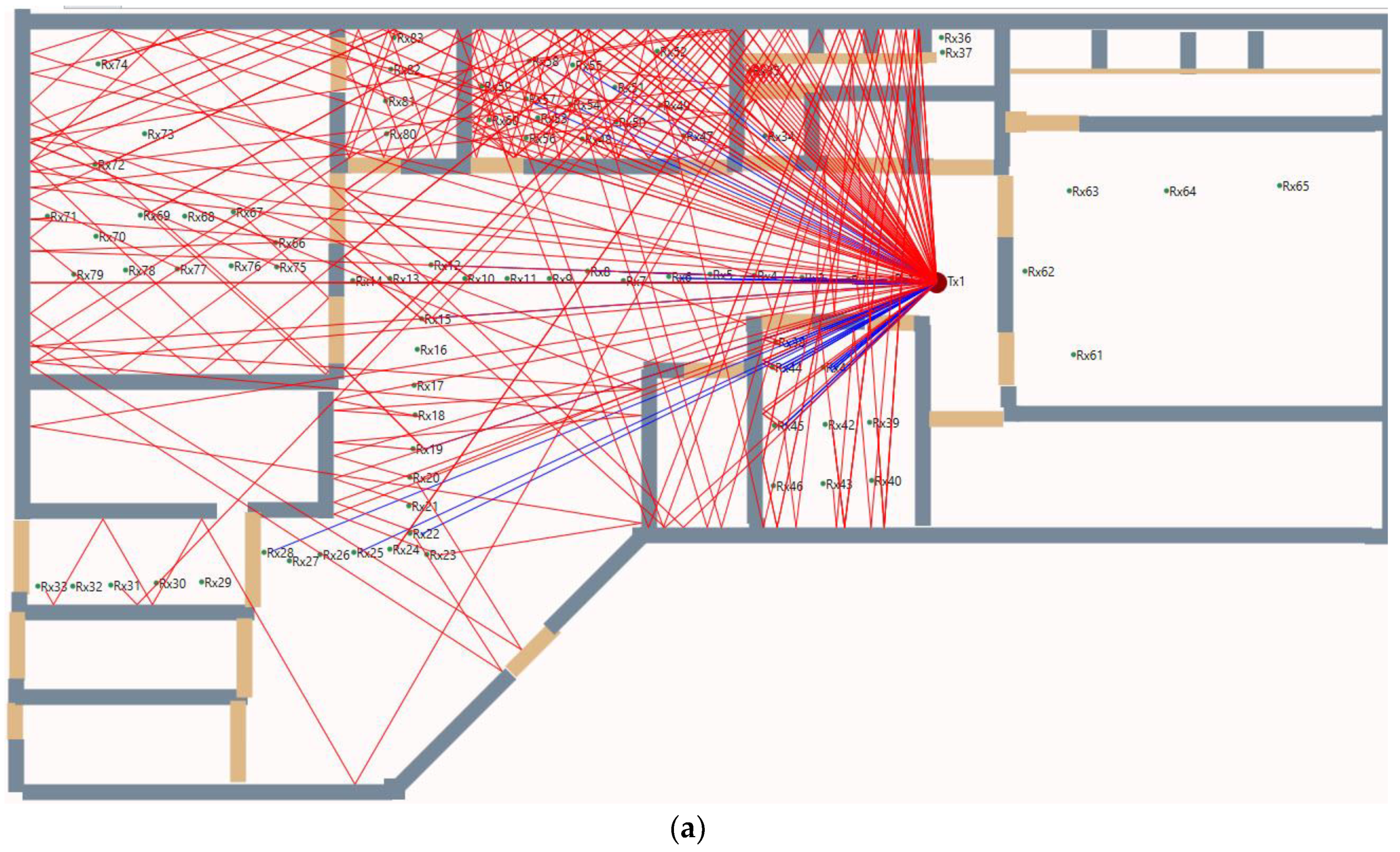
The measurement is performed using one Tx and 39 Rx points in the building. All mobile station points are placed among the LOS and NLOS criteria with the various distances of Tx–Rx between 1 and 22.7 m range. The floor lengths and widths are approximately 21 m and 30 m, respectively.
In the measurement procedure, first the Tx antenna is at a fixed position of Room 1 in the WCC P15a, as shown in
Figure 1. The measurement begins with the nearby Rx, which is 1 m away from Tx. The data are recorded along with the Rx fixed point at that position. The measurement procedure is re-run for each Rx point; also, Tx and Rx antennae are placed in the angular layout, where all data are recorded.
3. Hardware Specifications and Measurement Setup
The wireless base-station, model Anritsu MG369xC (Anritsu, Atsugi, Kanagawa Prefecture, Japan), is set up to generate continuous radio wave. The output of the radio frequency is connected with the directional horn antenna Tx. The vicinity of Rx point, the RSSI, and PL are quantified via linking Omni-directional base station to the MS2720T (Anritsu, Atsugi, Kanagawa Prefecture, Japan), a spectrum band analyzer. It operates at zero spans and frequency bandwidth of the spectrum band analyzer is constant at 100 kHz. The technical specifications of the hardware are given in
Table 1.
Here the Tx is a horn antenna and Rx is an omni-directional antenna. The transmitted power Pt is 25 dBm. The assessment setup uses factors stated in
Table 2.
4. Simulation Server Specifications and Parameter Configuration
In the RT simulation comparison with the measurement, the simulation channel uses the same parameter as in the measurement. However, a better system for simulation analysis uses a horn antenna for Tx and omnidirectional antenna for Rx. In simulation, Windows 64-bit server (Y0M88AA#UUF), Windows server 2016 OS version 10.0*, and processor core i7 are used. The RAM is 16.0 GB, with a 4-GB GDDR5 Graphics card. This simulator is developed with the programing language C# (WPF, VS 2017, version: 15.5.2) and database structured query language (SQL) server 2017 standard edition. In this research, the proposed method and SBRT method are similarly implemented in the in-house developed simulator. This simulator works dynamically based on some configurable parameters [
27,
28]. The common parameters for both algorithms are similarly incorporated in the simulation. The same relevant parameters are used in both simulations for measurement.
For the purpose of simulating signal generation, a horn 4.5-GHz Tx antenna is used, and placed at the coordinates of the Tx point in the layout scenario. The base station height plays a vital role in this simulation. Reflection relationally depends on Tx height; the higher Tx bears a lower number of interactions rather than that of the lower one. In this simulation, the Tx height is 1.5 m and the transmitter power is 25 dBm. For distance measurement, 80 pixels is considered a meter. In this simulation, interactions can be controlled by its limit; a maximum 25 reflections are considered for a single ray. The ray thickness is one pixel.
5. Proposed Ray Tracing Method
In the existing RT method, rays are emitted at random at all possible angles, and a 3-D RT is required for every ray. A ray may hit the target Rx point intersecting the Rx capture points, or it can be out because it does not touch the Rx point sphere. This process requires a large amount of resources, bearing high computational time. The proposed algorithm does not allow emission in all possible directions; rather, it allows only more rays to some zone where the Rx is situated. The development of the proposed 3D RT algorithm has seven steps:
Step I: 3-D Layout design and scenario creation.
Step II: 3-D ray emission with higher angle difference dimension based on the scenario.
Step III: Tracing of rays for successful directions by calculation.
Step IV: Specification of successful directions at nearby forward direction.
Step V: Specification of successful directions at nearby backward direction.
Step VI: Definition of wider directions 3-D RL faced on Steps III to V.
Step VII: Ray tracing at more successful ray directions.
In Step I, layout of the 3-D scenario is created by considering several obstacles, Tx, Rx, and the components in the environment.
In Step II, directional 3-D ray emission lets it propagate through the layout intersecting the objects, including interactions such as reflection, refraction, and diffraction. In this step, emission rays in the high vertical step size have small effects on the results. Hence, only the vertical angle difference θ = π/60 is used.
In Step III, pre-RT is performed base on the calculation, in order to identify the successive angles θ whose ray contributes to Rx.
In Step IV, at every successive vertical angle some forward direction rays are added to generate extra rays to the predefined potential zone. The direction step size based on the simulation scenario can be π/720, π/360, π/240, or π/180 radian from the successful angles. This step improves the coverage and the propagation time.
List<double> WiderVerticalAngles = new List<double> ();
if (SuccessiveVerticalAngles! = NULL)
{
WiderVerticalAngles.Add(SuccessiveVerticalAngles + π / 240);
WiderVerticalAngles.Add(SuccessiveVerticalAngles + π / 120);
}
In Step V, at every successive vertical angle, some backward directions ray are added to generate more rays to the predefined potential zone. The direction dimension based on the scenario, can be −π/720, −π/360, −π/240, or −π/180 radian from the successive angles. This step also improves the coverage and the propagation time.
List<double> WiderVerticalAngles = new List<double> ();
if (SuccessiveVerticalAngles! = NULL)
{
WiderVerticalAngles.Add(SuccessiveVerticalAngles - π / 120);
WiderVerticalAngles.Add(SuccessiveVerticalAngles - π / 240);
}
In Step VI, all directions received from Step III to Step V are combined, and made distinct.
List<double>FinalWiderVerticalAngles = WiderVerticalAngles.Distinct(). ToList();
In this way, all distinct direction emission rays will hit the Rx probable zone to make better coverage.
In Step VII, all emission rays are traced and lines drawn with color blue if LOS; or else, colored red if it is NLOS. The simulation results are saved in the database for further investigation.
5.1. Workflow of Proposed Method and SBRT Method
Figure 2 displays the workflow of the proposed RT method in (a) and the conventional SBRT in (b). The symbol N and M express the number of RL for preprocessing and successful directions, together with additional unique forward and backward directions. In the proposed 3-D RT method, vertical angle difference π/60 radian was used but in the conventional method π/180. In calculation, because of the vertical angle difference, the SBRT method launched three times more rays than the proposed RT method without sensing the Rx potential zone. However, the proposed 3-D RT method launches more rays finally in the potential zone after pre-sensing.
5.2. Complexity Analysis of the Proposed Method
The complexity of the proposed 3-D RT is low, because only pre-defined rays are finally launched. The lower number of launching rays give better accuracy even under a higher level of interactions. Moreover, less computational resources are needed handle this method. In the conventional methods, more rays are shot in all directions, so the complexity of the calculation increases massively. However, the shooting of massive ray’s object touching calculations are needed to perform blindly without knowing whether it contributes to Rx or not. Our method uses less time and, therefore, less computational complexity. This method simulation time is equal to . The symbol , , , and t are RL horizontal angle step size, RL vertical angle step size, RL horizontal angle range, RL vertical angle range, number of successful directions in pre-calculation in Step III, and average simulation time (ns) for a ray, respectively. For an omnidirectional base station, value is 0 to 360 degrees; it is divided by launching horizontal step resolution as it launches the rays in a 360-degree angle but for horn antenna, it is controlled by the beam width. Here, the RL horizontal step size () reduces the number of launching rays in Step III drastically. Moreover, in this method, more RL can be ensured in the pre-calculated identified zone. In the conventional method, has several values, such as , , and these values rapidly increase the number of launching rays.
6. Ray Tracing Modeling Calculations
In indoor radio propagation, a ray may face multiple reflections, transmissions, and diffractions before reaching an Rx. From the statement, an electric field intensity
can be written as Equation (1) [
29].
Here, is the incident electric field for the first scattering point. The are the number of reflections, transmissions, and diffractions that occurred one after another. The express the associate dyadic reflections, transmissions, and diffraction coefficients, respectively. The express the related spreading factors, and Sn is the total distance the ray travels.
Generally, because of multi-path propagation, Rx will receive more than one ray. For this scenario, the total electric field intensity, E
total is the adjacent summation of every ray, as given by Equation (2).
where M is the total number of rays reaching the receiver. Getting the value of transmitting power from the base station (
), antenna pattern, and polarization and
from RT
can be calculated using Equation (3).
Here
expresses the electric field intensity at the 1 m distance from the Tx in the direction of maximum antenna gain [
30]. The
mean intrinsic impedance around 120
,
is antenna directivity,
is the normalized antenna gain in the direction of
.The
expresses antenna polarization in the direction of
.The
is the distance of
from Tx.
Here
expresses only the ray field strength with respect to Rx. The actual measured voltage (
Vrn) is dependent on the Rx antenna type and the polarization. Assuming ideal and linear antennas and matched Rx, we write
Vrn as Equation (4).
Here,
expresses the wavelength;
, the Rx directivity in the ray arrival direction;
, the Rx characteristic impedance;
the receiving antennae polarization in the ray arrival direction; and
, the phase shift introduced by receiving antennae. Hence, the total received power RSSI is given by Equation (5) [
31].
Here, M is the total numbers of valid paths. In the path loss (PL) calculation for both the direct and indirect rays, we used Equation (6).
In Equation (6),
stands for path PL exponent, and
expresses zero mean Gaussian arbitrary variable with respect to standard deviation
. However, free space path loss
in free space PL for 1 m distance, is given by Equation (7).
where
stand for the operating frequency and the speed of visible light, respectively.
7. Validation of Ray Tracing Modeling Results
In this section, the detailed descriptions of the RT simulation and validation of RT with respect to actual measurement are presented. The purpose of the RT simulation is to validate the Rx position and measurement from the same Tx position. The indoor environment of an experimental area includes dimensional design by the 3-D RT tool, which also includes the environmental architecture and building features. The RT simulation is performed using the SBRT and proposed methods by the developed software. The RT features the maximum number of the ray interaction with the obstacles and indoor walls. Once a ray hits something, it starts reflecting; ray-tracing limits the maximum number of interactions. For each multipath, the RT considers the effects of reflections, and penetrations based on the GO and UTD. The simulation estimates the electromagnetic field according to the different rays received at the Rx point and calculates the results in the form of RSSI, PL [
32]. It is based on the 4.5 GHz propagation mechanism of indoor to trace paths up to the maximum PL; −150 dB is considered the minimum received sensitivity for RT simulation. If any of the interactions number reaches the maximum limit or the signal strength drops below the minimum receiver sensitivity, then this ray is ignored in the tracing. The high computation of RT simulation limits the interactions set to a considerable range to avoid dramatic changes in results. If all extents of propagation mechanisms are considered, the RT is not able to execute all propagation effects; or else the RT simulation requires a huge computation effort.
In this work, the measurement at WCC P15a and simulation performed on the layout use both the RT methods for indoor radio wave propagation. The layout scenario is designed with the in-house developed RT software for simulation. For the simulation, a simple model of layout is used, where only the main features are considered. Only normal windows and doors, transparent windows, and doors, and walls are incorporated. All other small obstacles are removed to simplify the layout. This simulation is performed to show how similar obstacles in the environment affect the results. The RT simulation has performed accurately in order to assess permittivity standards of some of the indoor obstacles in this layout as per measurement. Some practical difficulties are found in measuring the permittivity in obstacles, such as wooden walls, the different types of concrete in the floor, and the physical properties of the ceiling. Therefore, standard values of objects in [
33] are incorporated in the simulation.
This layout is designed and based on the UTM, WCC P15a, considering several big rooms.
Figure 3 shows the 2-D layout of design of the WCC P15a. The Tx is placed in the nearby Room 1. Several Rx are placed in different places, same as the measurement conducted. The indoor environment materials properties are directly related to the frequency spectrum. The parameters, such as dielectric constant and conductivity, are based on the material properties at different frequency bands [
34,
35,
36]. The simulation is performed using frequency dependent values of the dielectric constant and conductivity parameters at 4.5 GHz.
Figure 4 shows the graphical output of the present layout simulation using the SBRT method in 2-D and 3-D views. As shown, there are a large number of interactions; so, the PL, and the propagation durations are high and RSSI is low. Moreover, the mobile station coverage is not so stable because only a relatively lower number of rays reach the destination Rx. The fewer number of rays that reach the Rx, the weaker the signal strength. Although, some Rx receive more rays, most of those are from higher interactions, which bear high PL that have the direct effect on RSSI. As per simulation and measurement, output data with respect to RSSI and PL are found to have moderate similarity with the SBRT method.
Figure 5 shows the graphical output of the present simulation using the proposed RT method in 2-D and 3-D views. It shows fewer number of interactions, so PL, and the propagation time are low but the RSSI is high. It is also visible that the coverage is stable because a large number of rays reach the Rx, bearing a lower number of interactions. If more rays reach Rx, the signal strength will be accurate. Here, some Rx’s receive more rays but most of those bear fewer interactions and have low PL to have the direct positive impact on RSSI. As per simulation and measurement, output data with respect to RSSI and PL are found to have good agreement.
The average difference of RSSI between measurement and RT simulation using SBRT is 6.35 dBm for this scenario. The maximum and minimum difference of RSSI between the measurement and RT simulation using SBRT are 16.25 dBm and 0.1 dBm, respectively. The maximum RSSI difference takes place because of the suddenly appearing obstacles and the huge number of reflected rays. To see overall RSSI error for SBRT method with respect of measurement using Standard Deviation (SD) with a value of 4.23.
Similarly, the average difference of RSSI between measurement and RT simulation using the proposed method is 4.55 dBm for this scenario. The difference between measurement and simulation under five dBm is considered acceptable modeling. The maximum and minimum of RSSI differences between the measurement and RT simulation using the proposed method are 10.07 dBm and 0.23 dBm, respectively. However, the maximum difference takes place because of the sudden appearance of obstacles or reception of more reflected rays. Overall RSSI error as SD is 3.16 for the proposed method with respect to measurement. For the proposed method, even in an obstructed scenario, the difference in RSSI between measurement and proposed simulation is quite considerable.
Here, the measurement data are considered the standard data. The smaller value of SD expresses the lower error and higher accuracy of the method. Therefore, the overall RSSI SD value of proposed method is 1.07 less in compare to the SBRT method. From the RSSI comparison point of view with respect to data analysis, it is clear that the proposed method output demonstrates better agreement with measurement data compared with the SBRT output data.
PL reduces the electromagnetic signal strength as it travels through the path. PL is a major component to the indoor WCS analysis. The average difference of PL between measurement and RT simulation using SBRT is 6.01 dB for this scenario. The maximum and minimum difference of PL between the measurement and RT simulation using SBRT method are 24.05 dB and 1.45 dB, respectively. Overall PL error as SD is 4.91 for SBRT method with respect to measurement.
The maximum PL difference is due to the sudden appearance of obstacles or the huge number of reflected rays. The comparison of the PL between measurement and SBRT simulation with respect to several Rx from several locations is presented in
Table 3.
The average difference of PL between the measurement and RT simulation using the proposed method is 5.38 dB for this scenario. The maximum and minimum difference of PL between the measurement and RT proposed method simulation are 10.16 dB and 1.39 dB, respectively. Overall PL error as SD is 2.69 for the proposed method with respect to measurement. However, the maximum PL difference takes place because of the sudden appearance of obstacles or the huge number of reflected rays. Moreover, for the proposed method, even in obstructed scenarios, the difference in PL between measurement and the proposed method simulation is quite considerable. The comparison of the PL between proposed RT simulation and measurement with respect to several Rx from different locations is presented in
Table 3.
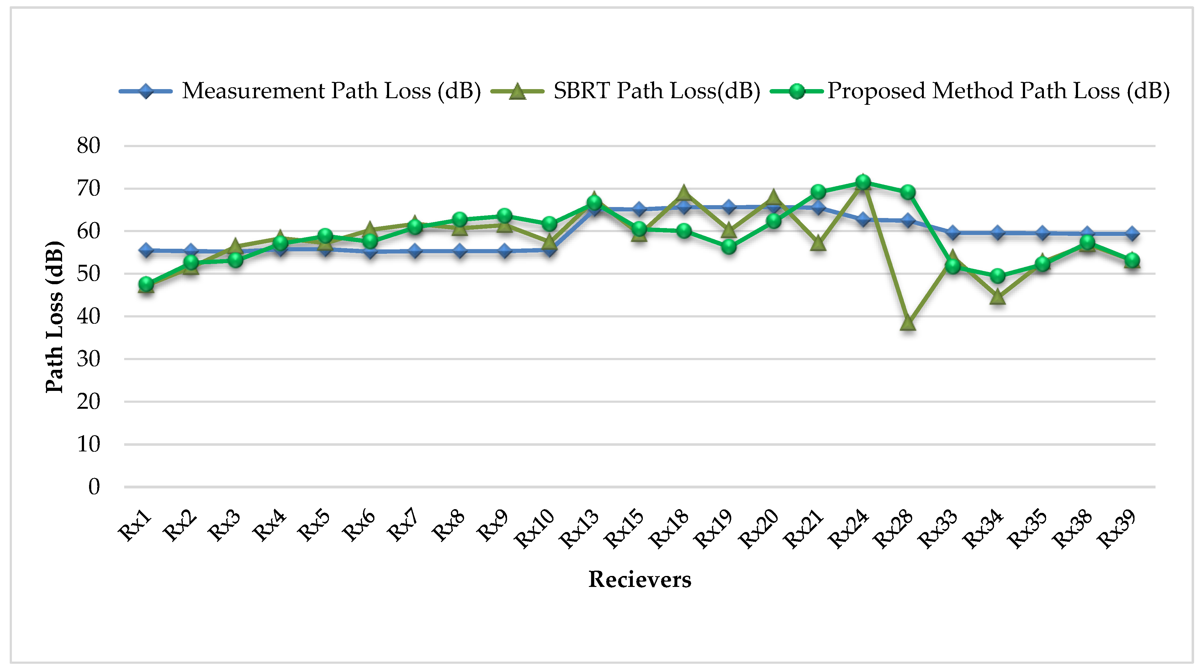
Figure 6 shows the graphical view of PL comparison among three sets of outputs data. Here, the measurement data are considered the standard data, which will help to validate the RT simulation. Consider the PL similarity trend of SBRT method: mobile stations Rx3, Rx5, Rx10, Rx13, Rx20, Rx38, Rx4, Rx18, and Rx2 demonstrate the moderate match with the measurement data, respectively. The average difference of PL from the measurement data to SBRT method data for those points is 2.33 dB. On the other hand, in the SBRT method, mobile stations Rx8, Rx19, Rx15, Rx33, Rx9, Rx39, Rx7, Rx35, Rx1, Rx21, Rx24, Rx34, and Rx28 demonstrate the distance relationship of PL respectively from the measurement data because of reflections. The average difference of PL from the measurement data to SBRT method data for those mobile stations is 8.38 dB. Even for some mobile stations, such as Rx8 near to Tx, comparative PL difference is high because of the large number of interactions. Again, according to the lower PL similarity trend of the proposed method, mobile stations Rx4, Rx13, Rx3, Rx38, Rx6, Rx2, Rx5, Rx20, Rx21, and Rx15 respectively demonstrate the good relationship with the measurement data. The average PL difference from the measurement data to proposed method data for those mobile stations is 2.65 dB. On the other hand, in the proposed method, mobile stations Rx18, Rx7, Rx10, Rx39, Rx28, Rx35, Rx8, Rx1, Rx33, Rx9, Rx24, Rx19, and Rx34 demonstrate distance relationship consecutively of PL from the measurement data, because of reflections. The average difference of PL from the measurement data to proposed method data for those mobile stations is 7.48 dB. Even some mobile stations such as Rx7 is nearby Tx, but comparative PL difference is high because of some large reflections.
Here, if we consider the more similar simulation as bearing the average PL difference with measurement data below 5 dB, 9 receivers are found in the SBRT method and 10 receivers are found in the proposed method. One other hand, if we consider the less similar simulation bearing the average PL difference with measurement data above 5 dB, 14 receivers are found in SBRT method, 13 receivers are found in the proposed method. Finally, the overall PL SD value of the proposed method is 2.69 less in comparison to the SBRT method. It expresses greater accuracy of the proposed method over the SBRT method. From the PL comparison points of view with respect to data analysis and
Figure 6, it is clear that in the proposed method, PL demonstrates more agreement with measurement data compared with the SBRT method.
The best RL plays a dynamic role in ray RT [
37,
38,
39,
40,
41,
42]. RL is the initial step of RT method. Therefore, the best use of the RL phase makes the proposed method more efficient, adaptive, and appropriate. The number of ray launchings needed for the proposed method is much fewer than that in the SBRT method. To get good coverage, using RL potential zone is the main key contribution of the proposed method. Hence, based on the stable coverage, good PL, lower propagation time, good RSSI, and best RL, the proposed method demonstrates a good contribution in WCS.
8. Conclusions
In this paper, a 3-D RT method for 4.5-GHz indoor radio propagation prediction has been proposed. It is a smarter, more effective way to categorize radio wave propagation for indoor scenarios using computerized simulation tools. Here, the RT used for the simulation purpose adopts two individual algorithms, the SBRT and the proposed efficient method. In this simulation, similar features of the layout, obstacle attenuation values, and antenna patterns are used as in the measurement. In general, it is difficult to get all values of the measurement and simulation to match the requirements of RSSI and PL. Moreover, the overall statistics of the measurement and simulation values with respect to RSSI and PL are reasonably similar. The proposed method output demonstrates more similarity with measurement than with conventional SBRT. The reduction of the PL SD from 4.91 dB for SBRT to 2.69 dB for the proposed method is significant contribution of proposed method. The comparison results show that the proposed RT is more accurate with respect to RSSI and PL. The proposed method achieves a noticeable gain in terms of computational efficiency by delivering more accurate RSSI and PL with respect to the standard measurement data.

 ,
, 


