Abstract
The examination of Personal Protective Equipment (PPE) to assure the complete integrity of health personnel in contact with infected patients is one of the most necessary tasks when treating patients affected by infectious diseases, such as Ebola. This work focuses on the study of machine vision techniques for the detection of possible defects on the PPE that could arise after contact with the aforementioned pathological patients. A preliminary study on the use of image classification algorithms to identify blood stains on PPE subsequent to the treatment of the infected patient is presented. To produce training data for these algorithms, a synthetic dataset was generated from a simulated model of a PPE suit with blood stains. Furthermore, the study proceeded with the utilization of images of the PPE with a physical emulation of blood stains, taken by a real prototype. The dataset reveals a great imbalance between positive and negative samples; therefore, all the selected classification algorithms are able to manage this kind of data. Classifiers range from Logistic Regression and Support Vector Machines, to bagging and boosting techniques such as Random Forest, Adaptive Boosting, Gradient Boosting and eXtreme Gradient Boosting. All these algorithms were evaluated on accuracy, precision, recall and score; and additionally, execution times were considered. The obtained results report promising outcomes of all the classifiers, and, in particular Logistic Regression resulted to be the most suitable classification algorithm in terms of score and execution time, considering both datasets.
1. Introduction
Highly infectious diseases are treated by very strict procedures following the advice of the World Health Organization (WHO) [1]. In the case of the Ebola virus, which has approximately 90% fatality rate, the protocol for both the patient and the medical staff results to be even more severe [2]. These security measures must guarantee an adequate protection of the worker and to the rest of the persons susceptible to direct or indirect contact with the patient and/or the worker. Several analysis have been performed to certify the efficiency of Personal Protective Equipment (PPE) to prevent the contamination with the infected patient [3], for example utilizing fluorescent markers [4,5]. Furthermore, Kang et al. [6] reported how significant it is to be aware and adopt standard procedures, demonstrating that frequent contaminations are related with lack of knowledge and carelessness of the health personnel. Other factors that could affect the performance of the PPE are related to a prolonged time wearing the equipment [7] or physical requirements such as the dimension of the changing room [8]. One of the most delicate tasks is the removal of the PPE in the changing room after visiting the patient [9]. The PPE that is used for treating this category of patients is composed by: (a) a protective suit that covers the entire body except face, hands, and feet; (b) FFP3 mask [10]; (c) waterproof glasses; (d) head cover; (e) three pairs of gloves; (f) two pairs of boot covers; (g) facial screen and body apron; and (h) areas of layer overlap (such as glove and suit on the forearm, and boot cover and suit on the legs) that are sealed with wide insulating adhesive tape.
The removal task involves several steps. During this activity, the actuation protocol states [11]: “We will always act slowly, calmly, being aware of our body and proceeding with slow but precise movements. Even feeling that we are accustomed to this activity, we will never stop listening and attending to the indications of the instructor-observer, which will indicate to the personnel the sequence for the removal of the PPE”. The first pair of gloves, as well as the first pair of boot covers, are discarded in the patient’s room. Gloves are always disposed, while other components are stored for their posterior sterilization and reuse. Once in the changing room, the steps that must be followed are reported in order: (1) remove the second pair of boot covers; (2) remove the second pair of gloves; (3) open the front closure of the suit; (4) remove the suit head cover, remove the suit arms and legs, remove completely and roll it up for storage; (5) remove the third pair of gloves; (6) perform first-hand hygiene; (7) put on a new pair of gloves; (8) remove the waterproof glasses; (9) remove the FFP3 mask; and (10) remove the new pair of gloves [11]. Figure 1 illustrates the removal of the second pair of gloves once inside the changing room.
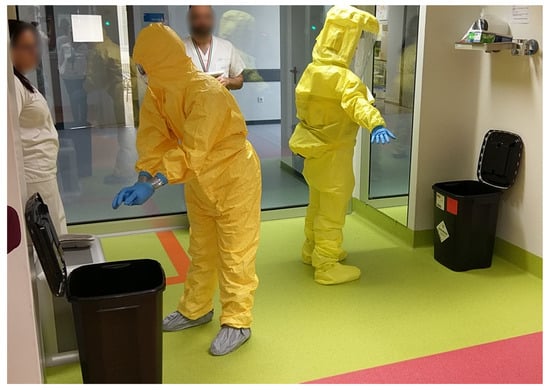
Figure 1.
Removal and disposal of gloves inside the changing room (during training session).
The possibility that the suit has been deteriorated and/or contaminated with traces of blood, vomit, urine and, in general, with various fluids may occur successive to the contact with infected patient. This fact can lead to worker contamination; therefore, a safe inspection of the protective equipment is necessary before proceeding with the removal task. The anomalies of the suit can be detected either by the health worker or by the instructor-observer (outside the changing room). However, visual inspection performed by humans results to be subjective, and may be affected by degree of expertise as well as circumstances such as distraction caused by fatigue. For this reason, an objective solution is necessary to validate the integrity of the PPE, which is for the health care of patients with Ebola and other highly infectious diseases.
The goal of this work was to study machine vision algorithms for a real prototype to ensure that the PPE protective suit is neither broken nor contaminated with fluids. The system consists in robotic structure that displaces a camera in Cartesian coordinates providing different levels of zoom, effectively acting as a full-body scanner. This camera provides monocular images that are analyzed by computer vision algorithms to detect undesired traits on the suit, such as stains of blood from interaction with the patient. We studied the accuracy, precision, recall, and score of a set of computer vision algorithms which are used for this system.
2. Materials and Methods
The problem statement can be solved through the use of machine vision classification algorithms, where the purpose is to define if a particular image taken by the camera is recognized as suit with or without certain traits, such as blood stains. An assumption made is that the number of clean areas will significantly outnumber those that present blood stains, which in classification problems is known as class imbalance [12]. Preceding studies analyze different approaches to treat unbalanced datasets in several real-world conditions, such as medical diagnosis [13], customer churn prediction [14], fraud detection in banking operations, creditworthiness of a bank’s customers [15], detection of oil spills [16], and data mining [17]. Common techniques can be categorized into three groups: data pre-processing, algorithmic approaches, and cost-sensitive learning [18]. Data processing involves adjustments to obtain a more balanced distribution, respectively, over-sampling the minority class and/or under-sampling the majority class [19,20,21]. Algorithmic approaches implicate the development of algorithms such as classification algorithms, ensemble techniques, decision trees, and neural networks, which take the class imbalance into account [22,23,24]. Cost-sensitive learning combines both the aforementioned techniques considering different types of costs [25,26]. Several classification algorithms, as well as performance metrics that can be used in the presence of class imbalance, are explained in this section.
2.1. Classification Algorithms
A preliminary study was performed to identify machine vision classification algorithms suitable for blood stain detection. In 2002, Melody et al. [27] studied the performance of different classifiers, among which Logistic Regression and Neural Networks presented higher accuracy with respect to some others such as Multivariate Discriminant Analysis, Decision Trees, and k-Nearest Neighbors. Brown and Mues et al. [28] based their comparison on an imbalanced credit scoring dataset, from which it emerges that Decision Trees, k-Nearest Neighbors and Quadratic Discriminative Analysis resulted to be not appropriate in the case of strong imbalance; rather than these, Random Forests and Gradient Boosting reported better outcomes. Regarding decision making in the clinical field, Support Vector Machines (SVM) showed greater diagnostic accuracy compared to Multilayer Perceptron Neural Networks, Combined Neural Networks, Mixture of Experts, Probabilistic Neural Networks, and Recurrent Neural Networks [29]. More recent research in the field of agricultural environments indicated a greater performance of Support Vector Machines and Random Forests; moreover, Adaptive Boosting (AdaBoost) exhibited good generalization capability specifically in case of large sample sizes [30]. Li et al. [31] compared 15 classification algorithms and determined that most of the supervised algorithms could achieve high accuracies setting adequate parameters and utilizing appropriate training samples. Since most of the standard classification algorithms assume a balanced training dataset [32], to avoid the misclassification of the minority class (images with blood stains) as much as possible, it is necessary to adjust the model used by the classifier. Based on previous research, our study focused on six different classifiers.
2.1.1. Logistic Regression
Logistic Regression (Logit) is one of the classification algorithms that is most used in machine learning. It is very similar to Linear Regression with the difference that Linear Regression is used for regression rather than for classification, thus their loss functions are typically different. The logistic function, also called Sigmoid, is an S-shaped curve that can take any real-valued number and map the output into a value between 0 and 1, but never exactly at those limits [33]. Hence, a Logistic Regression model determines the probability that the input variables belong to one of the two classes:
where x are the input variables and is the parameter vector. Logit is a very efficient and widely used method, due to its low computational complexity and minimal risk of overfitting [34].
2.1.2. Support Vector Machine
Support Vector Machines (SVM) are supervised learning algorithms which can be utilized both for discriminative classification and regression problems. They are based on the definition of an optimal hyperplane (Figure 2). For classification, this hyperplane is identified by the maximum margin between the vectors of the two classes [35].

Figure 2.
Support Vector Machine hyperplane, in which blue spots are positive samples, pink spots correspond to the negative samples, the rimmed ones are the support vectors, and the central thicker line is the obtained optimal hyperplane [36].
The margin to obtain an optimal hyperplane is defined considering only a small set of the training data, called support vectors [35]. The SVM classifier works very well with a clear margin of separation and in high dimensional spaces, but also exhibits a prolonged time execution when there is a large dataset [37]. Furthermore, this classifier has been applied to several areas such as object detection [38], digital handwriting recognition [39], and text categorization [40,41].
2.1.3. Random Forest
Random forest (RF) is a decision tree classifier referred to an ensemble algorithm of supervised learning. This ensemble technique creates a set of decision trees from randomly selected subsets of training data [42]. The selected training data are the only ones used to find the best split for the node; in this way, each split is based on the best features among a random subset of features [43]. This kind of approach is called bagging and it involves parallel training of the different models. Moreover, considering the significant imbalance of our classes, it can be necessary to additionally adjust the class weight parameter to increase the weight of the minority class and obtain an equal percentage of the two classes. The advantages of using a Random Forest algorithm is that it can handle high dimensional data, perform large numbers of trees, and avoid overfitting [44,45].
2.1.4. Adaptive Boosting
The Adaptive Boosting (AdaBoost) is one of most efficient and widely used classifiers; moreover, it was the first successful boosting algorithm developed for binary classification introduced by Freund and Schapire [46]. The boosting technique involves the formation of a strong classifier from several weak classifiers, but here the weaker classifiers are created sequentially and not “in parallel” as in the bagging methods. Furthermore, AdaBoost adjusts the weight of the instances at each iteration, given more weight for the misclassified samples and less weight for the right ones. The number of weak learners can be regulated to obtain the best performance and usually the higher is the number of estimators the better will be results. The order of magnitude of weak learners used is typically between tens and hundreds of estimators. Based on previous studies, this classifier shows a very good generalization (the ability to classify new data) although some literature indicates it is not qualified to prevent overfitting when dealing with very noisy data [47].
2.1.5. Gradient Boosting
A different Boosting approach is called Gradient Boosting (GB) [48], which over the last few years has obtained a great interest. This learning procedure progressively fits new models to define the strong classifier [49]. The new model gradually minimizes the loss function; in such way, the initial base learner is grown and every tree in the series is fit to the pseudo-residuals of the prediction from the earlier tree [28]. The resulting formula is shown below:
where equals the first value for the series, are the trees fit to the pseudo-residuals, and are coefficients for the tree nodes computed by the algorithm [28]. The parameter that is possible to set up is the number of estimators, as well as the number of boosting stages to execute. The order of magnitude of estimators used is also typically between tens and hundreds. The GB classifier allows fast execution time and high accuracy [50]. The most common problem regarding these estimators is overfitting, which could arise depending on the choice of the weak learners or if the number of them reaches large values [51].
2.1.6. eXtreme Gradient Boosting
The last classifier of study is the eXtreme Gradient Boosting (XGB), which is a variation of the above-mentioned Gradient Boosting [52]. It involves a parallel tree boosting procedure to solve the classification problem and adds few levels of regularization to prevent the overfitting [53]. Likewise, the order of magnitude of estimators used with this classifier is typically between tens and hundreds. The XGB results to be highly efficient, flexible, simple and very fast due to a parallel implementation on the features [53].
2.2. Performance Metrics Analyzed
All the aforementioned classification algorithms were evaluated on four performance metrics: accuracy, precision, recall and score. These metrics can be obtained from the parameters reported in a confusion matrix (Figure 3):
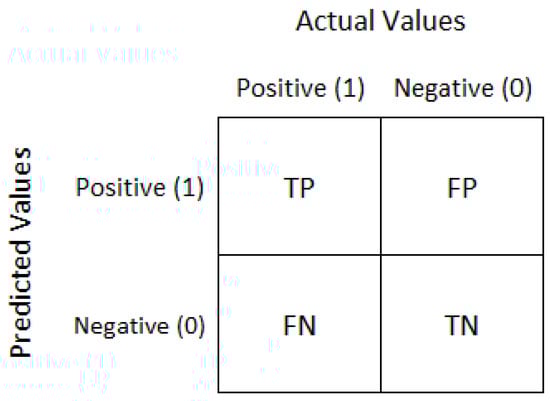
Figure 3.
The confusion matrix compares the predicted values with respect to the actual real values. In particular, the matrix elements are defined as: TP, true positive, the cases in which we predicted that there is blood and there is actually blood; TN, true negative, where we predicted there is no blood and there is no blood; FP, false positive, we predicted there is blood and instead there is no blood; and, FN, false negative, where we predicted there is no blood but there actually is blood.
Accuracy is defined as the percentage of correctly classified positive and negative samples on the total observation, and the formula is reported below [54]:
The second parameter is called precision and it is determined with number of positive predictions divided by the total number of positive samples values predicted [55]:
Recall, instead, is used to measure the fraction of positive samples that are correctly classified, thus is true positives samples divided by true positives plus false negatives [56]:
The last parameter is known as score, which is considered the weighted average of the precision and recall, as is it is possible to observe in the reported formula [54]:
These metrics have been provided as they jointly provide more insight on the performance of the classifiers. Specifically, accuracy may provide misleading results in the case of unbalanced data (e.g., a classifier that treats all samples as clean would report a high accuracy) [57], but its values can be better interpreted in the context of the other metrics.
3. Experimental Setup
The study involved an initial analysis on a synthetic image dataset, followed by an additional study on an image dataset of the PPE with a physical emulation of blood stains taken by a real prototype. Figure 4 illustrates the simulated PPE suit and the physical PPE that were used for our investigation. The datasets have been openly published as a specific complement of this work [58].

Figure 4.
Comparison between the PPE suit of the simulated environment (left) and the physical PPE suit in the actual full-body scanner mechanism (right).
3.1. Synthetic Dataset
The synthetic dataset was reconstructed with a simulated environment that includes the protective suit with the blood stains. The simulated environment additionally allows different points of illumination and zoom levels, as shown in Figure 5.
Figure 5.
Possible points of illumination can be chosen within the simulated environment.
This dataset includes 30 images of 960 × 480 pixels, taken with a fixed simulated focal length of 4.8 mm. These images represent the whole protective suit subdivided into six different areas (Figure 6): chest, abdomen, pelvis, thighs, lower legs and ankles. Five different synthetic samples were generated for each of the six areas, each with a different point of illumination. The total time required for rendering these 30 simulated images was 15.75 s. To represent the data distribution of the physically emulated dataset, the synthetic dataset is also affected by a strong imbalance between the two class samples, where the stained areas represent 0.0006% of the total of 13,824,000 pixels, and the majority represent clean areas.

Figure 6.
The full-body suit subdivided into six areas: chest, abdomen, pelvis, thighs, lower legs, and ankles.
3.2. Physical Emulated Dataset
The acquisition of images with physical emulation of blood stains was performed on a real PPE suit using a proprietary blood simulant and the actual full-body scanner mechanism of Figure 4. Images were obtained utilizing the system’s single monocular camera surrounded by four high intensity LED lamps and different camera focal length from 4.8 mm (0% zoom) to 57.6 mm (100% zoom) (Figure 7). The total time required for the acquisition was 19.23 min, dominated by camera movement times such that actual camera acquisition times are depreciable. This second dataset is composed by a larger number of images at higher resolution and a larger proportion of stains: 47 images of 1280 × 960 pixels, where stained areas represent a 2.25% of the total of 57,753,600 pixels.

Figure 7.
Physical emulated dataset respectively with different zoom levels: the (upper left) image represents 4.88 mm of focal length (0% zoom), the (upper right) image corresponds to 31.92 mm focal length (60% zoom), and the (bottom) image with focal length of 57.6 mm (100% zoom).
Such high intensity LED illumination technology provides information in a wide spectrum, ranging from UV to IR, in particular: (a) white light is used for blood stains, bruises and bites; (b) UV light for body fluids and drug residues; (c) violet light for splashing blood and hair; (d) orange and red light for general contrast search; and (e) IR light for blood splashes, fiber, etc. [59]. In view of the detection of exclusively blood stains, temporarily the white light was the only one utilized.
4. Experimental Results
In our study, six classification algorithms were trained on a synthetic and a physical emulated dataset. In particular, classifiers which are able to manage the high imbalance between the positive and negative samples were selected. Initially, Logistic Regression and a discriminative classification algorithm, known as Support Vector Machine, were carried out. The investigation further proceeded through the application of bagging and boosting approaches, in particular with the Random Forest for the bagging techniques and Adaptive Boosting, Gradient Boosting and eXtreme Gradient Boosting relative to the second approach. The performances of these classification algorithms were evaluated on the four metrics in Section 2.2, presented for the synthetic dataset in Table 1 and for the physical emulated dataset in Table 2.

Table 1.
Outcomes obtained on simulated PPE images from the six classifiers: Logistic Regression (Logit), Support Vector Machine (SVM), Random Forest (RF), Adaptive Boosting (AdaBoost), Gradient Boosting (GB) and eXtreme Gradient Boosting (XGB). All these learners were evaluated on four parameters: Accuracy (Acc), Precision (Pr), Recall (Re) and score; moreover, the execution time was taken into account ( in minutes).
Table 2.
Results acquired on real PPE images from the six classifiers: Logistic Regression (Logit), Support Vector Machine (SVM), Random Forest (RF), Adaptive Boosting (AdaBoost), Gradient Boosting (GB) and eXtreme Gradient Boosting (XGB). All these learners were evaluated on four parameters: Accuracy (Acc), Precision (Pr), Recall (Re) and score; moreover, the execution time was taken into account ( in minutes).
From the results presented in Table 1 and Table 2, is possible to observe that all the classifiers exhibit positive results. To define the classification algorithm that better approximates the desired outcomes, several aspects of each metric parameters were taken into account. Firstly, for the accuracy, which is the ratio of correctly predictive observations respect to the total observations, the best values were reported from the Support Vector Machine with 99.99% for the synthetic dataset, and from the eXtreme Gradient Boosting with 99.23% using 200 estimators for the physical emulated dataset. Regarding this metric parameter, it is important to specify that, in our particular condition, it is not the appropriate measure for model performance evaluation. In fact, when facing strongly imbalanced datasets, accuracy values may result misleading, as explained in Section 2.2. Considering the precision, the highest values for both datasets were reported from Adaptive Boosting, with, respectively, 100% on the synthetic PPE images utilizing 30 estimators, and 95.77% on the physical emulated blood stains dataset with 50 estimators.
This metric takes false positives into account, which are instances that our model incorrectly recognized pixels as blood stain that are actually clean areas. On the other hand, recall considers false negatives, which are cases in which our model labels pixels as clean areas where instead blood stains are present. Therefore, when precision increases, recall decreases, and vice versa. It is possible to observe this in the case of Adaptive Boosting, which presented the maximum precision values, but in terms of recall resulted to be one of the worst classification algorithm for both datasets. For this reason, a trade off between these two parameters is necessary and this is called the score. The aforementioned metric is a weighted average of precision and recall. Combining these two terms results to be the best measure for our performance evaluation. The highest outcomes were obtained from the Support Vector Machine with 98.82% for the synthetic dataset, and eXtreme Gradient Boosting utilizing 200 estimators with 80.68% for the physical emulated dataset. The execution time was the last compared measurement among all the algorithms; furthermore, in our study, it is important to consider that the two dataset were performed on two different machines. The first dataset, which includes synthetic images, was executed on a standard 3.00 GHz dual-core CPU machine, while the second larger dataset, composed by larger real PPE images, was treated on a 4.00 GHz quad-core CPU machine with an NVIDIA Titan X GPU. The fastest algorithms regarding the first dataset were Logistic Regression and eXtreme Gradient Boosting (with 20 estimators), both performing within 2 min. The processing of physical emulated PPE images needs more time; in fact, here, both Logistic Regression and eXtreme Gradient Boosting executed approximately around 5 min. Moreover, it is possible to observe in Table 2 that the SVM did not achieve any results after more than one week of processing the emulated blood stains (over 10,080 min).
5. Conclusions
In this study, several classification algorithms were compared, from conventional Logistic Regression to more modern algorithms such as eXtreme Gradient Boosting, to detect undesired blood stains on the personal protective suit of medical care personnel after contact with infected patients. The analysis involves the evaluation of the algorithms on two datasets: the first includes synthetic images of the PPE that were reconstructed in a simulated environment, and the second represents images of the PPE with physical emulated blood stains acquired through a real prototype. All the classifiers were evaluated on four performance metrics and taking their execution time into account. From the obtained results, it is possible to observe that all the selected algorithms report satisfying outcomes (above 50%); furthermore, as we expected, the physical emulated images are more challenging to be processed and this may be due to irregular blood stains or a larger dataset. For the definition of the most suitable algorithm, it was necessary to consider the great imbalance between the positive and negative class samples. In this condition, the score results to be the most appropriate metric parameter. In particular, the highest values were reported from Support Vector Machine for the first images dataset and from the eXtreme Gradient Boosting for the second dataset; in both cases, prolonged execution times were needed. Therefore, the best solution was to find a compromise between score and execution time , where Logistic Regression achieved the most balanced outcomes considering both datasets.
Author Contributions
Conceptualization, A.S., J.G.V. and D.E.; Data curation, A.S. and D.E.; Formal analysis, J.G.V.; Funding acquisition, C.B.; Investigation, A.S., J.G.V. and D.E.; Methodology, A.S. and D.E.; Project administration, J.G.V. and C.B.; Resources, C.B.; Software, A.S., J.G.V. and D.E.; Supervision, J.G.V. and C.B.; Validation, A.S.; Visualization, J.G.V.; Writing—original draft, A.S.; and Writing—review and editing, J.G.V. and C.B.
Funding
The research leading to these results received funding from: Inspección robotizada de los trajes de proteccion del personal sanitario de pacientes en aislamiento de alto nivel, incluido el ébola, Programa Explora Ciencia, Ministerio de Ciencia, Innovación y Universidades (DPI2015-72015-EXP); the RoboCity2030-DIH-CM Madrid Robotics Digital Innovation Hub (“Robótica aplicada a la mejora de la calidad de vida de los ciudadanos. fase IV”; S2018/NMT-4331), funded by “Programas de Actividades I+D en la Comunidad de Madrid” and cofunded by Structural Funds of the EU; and ROBOESPAS: Active rehabilitation of patients with upper limb spasticity using collaborative robots, Ministerio de Economía, Industria y Competitividad, Programa Estatal de I+D+i Orientada a los Retos de la Sociedad (DPI2017-87562-C2-1-R).
Conflicts of Interest
The authors declare no conflict of interest.
References
- World Health Organization. Ebola Situation Report-8 April 2015. Available online: http://apps.who.int/ebola/current-situation/ebola-situation-report-8-april-2015 (accessed on 21 June 2019).
- World Health Organization (Regional Office for Europe). Antimicrobial Resistance-Data and Statistics. Available online: https://web.archive.org/web/20170318012903/http://www.euro.who.int/en/health-topics/disease-prevention/antimicrobial-resistance/data-and-statistics (accessed on 21 June 2019).
- Mayer, A.; Korhonen, E. Assessment of the Protection Efficiency and Comfort of Personal Protective Equipment in Real Condition of Use. Int. J. Occup. Saf. Ergon. 1999, 5, 347–360. [Google Scholar] [CrossRef][Green Version]
- Bell, T.; Smoot, J.; Patterson, J.; Smalligan, R.; Jordan, R. Ebola virus disease: The use of fluorescents as markers of contamination for personal protective equipment. IDCases 2015, 2, 27–30. [Google Scholar] [CrossRef][Green Version]
- Hall, S.; Poller, B.; Bailey, C.; Gregory, S.; Clark, R.; Roberts, P.; Tunbridge, A.; Poran, V.; Evans, C.; Crook, B. Use of ultraviolet-fluorescence-based simulation in evaluation of personal protective equipment worn for first assessment and care of a patient with suspected high-consequence infectious disease. J. Hosp. Infect. 2018, 99, 218–228. [Google Scholar] [CrossRef]
- Kang, J.; O’Donnell, J.; Colaianne, B.; Bircher, N.; Ren, D.; Smith, K. Use of personal protective equipment among health care personnel: Results of clinical observations and simulations. Am. J. Infect. Control 2017, 45, 17–23. [Google Scholar] [CrossRef]
- Loibner, M.; Hagauer, S.; Schwantzer, G.; Berghold, A.; Zatlouk, K. Limiting factors for wearing personal protective equipment (PPE) in a health care environment evaluated in a randomised study. PLoS ONE 2019. [Google Scholar] [CrossRef]
- Gao, P.; King, W.; Shaffer, R. Review of chamber design requirements for testing of personal protective clothing ensembles. J. Occup. Environ. Hyg. 2007, 4, 562–571. [Google Scholar] [CrossRef]
- Lim, S.; Cha, W.; Chae, M.; Jo, I. Contamination during doffing of personal protective equipment by healthcare providers. Clin. Exp. Emerg. Med. 2015, 2, 162–167. [Google Scholar] [CrossRef]
- European Committee for Standardization (CEN). Respiratory Protective Devices—Filtering Half Masks to Protect Against Particles—Requirements, Testing, Marking; European Standard EN 149:2001 + A1:2009; CEN: Rome, Italy, 2018; Available online: https://eur-lex.europa.eu/legal-content/EN/TXT/HTML/?uri=OJ:C:2018:209:FULL (accessed on 21 June 2019).
- Ministerio de Sanidad, Servicios Sociales e Igualdad. Protocolo de Actuación Frente a Casos Sospechosos de Enfermedad por Virus Ébola (EVE). 2015. Available online: http://www.mscbs.gob.es/profesionales/saludPublica/ccayes/alertasActual/ebola/documentos/16.06.2015-Protocolo_Ebola.pdf (accessed on 21 June 2019).
- Japkowicz, N. The Class Imbalance Problem: Significance and Strategies; Faculty of Computer Science DalTech, Dalhousie University 6050 University: Halifax, NS, Canada, 2000. [Google Scholar]
- Rahman, M.M.; Davis, D.N. Addressing the Class Imbalance Problem in Medical Datasets. Int. J. Mach. Learn. Comput. 2013, 3, 224. [Google Scholar] [CrossRef]
- Burez, J.; Van den Poel, D. Handling class imbalance in customer churn prediction. Expert Syst. Appl. 2006, 36, 4626–4636. [Google Scholar] [CrossRef]
- Huanga, Y.; Hunga, C.; Jiaub, H. Evaluation of neural networks and data mining methods on a credit assessment task for class imbalance problem. Nonlinear Anal. Real World Appl. 2006, 7, 720–747. [Google Scholar] [CrossRef]
- Kubat, M.; Holte, R.; Matwin, S. Machine learning for the detection of oil spills in satellite radar images. Mach. Learn. 1998, 30, 195–215. [Google Scholar] [CrossRef]
- Longadge, R.; Dongre, S.; Malik, L. Class Imbalance Problem in Data Mining: Review. arXiv 2013, arXiv:1305.1707. [Google Scholar]
- López, V.; Fernández, A.; García, S.; Palade, V.; Herrera, F. An insight into classification with imbalanced data: Empirical results and current trends on using data intrinsic characteristics. Inf. Sci. 2003, 250, 113–141. [Google Scholar] [CrossRef]
- Estabrooks, A.; Jo, T.; Japkowicz, N. A Multiple Resampling Method For Learning From Imbalanced Data Sets. Comput. Intell. 2004, 20, 18–36. [Google Scholar] [CrossRef]
- Lewis, D.; Catlett, J. Heterogeneous Uncertainty Sampling for Supervised Learning. In Machine Learning, Proceedings of the Eleventh International Conference, New Brunswick, NJ, USA, 10–13 July 1994; Rutgers University: New Brunswick, NJ, USA, 1994; pp. 148–156. [Google Scholar]
- García, V.; Sánchez, J.; Mollineda, R. On the effectiveness of preprocessing methods when dealing with different levels of class imbalance. Knowl.-Based Syst. 2012, 25, 13–21. [Google Scholar] [CrossRef]
- Galar, M.; Fernandez, A.; Barrenechea, E.; Bustince, H.; Herrera, F. A Review on Ensembles for the Class Imbalance Problem: Bagging-, Boosting-, and Hybrid-Based Approaches. IEEE Trans. Syst. Man Cybern.-Part C Appl. Rev. 2011, 42, 463–484. [Google Scholar] [CrossRef]
- Haixianga, G.; Yijinga, L.; Shang, J.; Mingyuna, G.; Yuanyuea, H.; Binge, G. Learning from class-imbalanced data: Review of methods and applications. Expert Syst. Appl. 2017, 73, 220–239. [Google Scholar] [CrossRef]
- Dai, W.; Brisimi, T.; Adams, W.; Melac, T.; Saligramaa, V.; Paschalidis, I. Prediction of hospitalization due to heart diseases by supervised learning methods. Int. J. Med. Inform. 2015, 84, 189–197. [Google Scholar] [CrossRef]
- Ling, C.; Sheng, V. Cost-Sensitive Learning and the Class Imbalance Problem. In Encyclopedia of Machine Learning; Sammut, C., Ed.; Springer: Berlin/Heidelberg, Germany, 2008. [Google Scholar]
- Weiss, G.; McCarthy, K.; Zabar, B. Cost-Sensitive Learning vs. Sampling: Which Is Best for Handling Unbalanced Classes with Unequal Error Costs? Department of Computer and Information Science Fordham University Bronx: Bronx, NY, USA, 2017. [Google Scholar]
- Kiang, M. A comparative assessment of classification methods. Decis. Support Syst. 2003, 35, 441–454. [Google Scholar] [CrossRef]
- Brown, I.; Mues, C. An experimental comparison of classification algorithms for imbalanced credit scoring data sets. Expert Syst. Appl. 2012, 39, 3446–3453. [Google Scholar] [CrossRef]
- Ubeyli, E. Comparison of different classification algorithms in clinical decision-making. Expert Syst. 2007, 24, 17–31. [Google Scholar] [CrossRef]
- Li, M.; Ma, L.; Blaschke, T.; Cheng, L.; Tiede, D. A systematic comparison of different object-based classification techniques using high spatial resolution imagery in agricultural environments. Int. J. Appl. Earth Obs. Geoinf. 2016, 49, 87–89. [Google Scholar] [CrossRef]
- Li, C.; Wang, J.; Wang, L.; Hu, L.; Gong, P. Comparison of Classification Algorithms and Training Sample Sizes in Urban Land Classification with Landsat Thematic Mapper Imagery. Remote Sens. 2014, 6, 964–983. [Google Scholar] [CrossRef]
- Branco, P.; Torgo, L.; Ribeiro, R.A. Survey of Predictive Modelling under Imbalanced Distributions; LIAAD-INESC-TEC, DCC-Faculdade de Ciencias, Universidade do Porto: Porto, Portugal, 2015. [Google Scholar]
- Stoltzfus, J. Logistic Regression: A Brief Primer. Res. Methods Stat. 2011, 18, 1099–1104. [Google Scholar] [CrossRef] [PubMed]
- Dreiseitla, S.; Ohno-Machadob, L. Logistic regression and artificial neural network classification models: A methodology review. J. Biomed. Inform. 2002, 35, 352–359. [Google Scholar] [CrossRef]
- Cortes, C.; Vapnik, V. Support-Vector Networks. Mach. Learn. 1995, 20, 273–297. [Google Scholar] [CrossRef]
- Isozaki, H.; Kazawa, H. Efficient Support Vector Classifiers for Named Entity Recognition; NTT Communication Science Laboratories Nippon Telegraph and Telephone Corporation: Kyoto, Japan, 2002. [Google Scholar]
- Rejab, F.; Nouira, K.; Trabelsi, A. RTSVM: Real Time Support Vector Machines. In Proceedings of the 2014 Science and Information Conference, London, UK, 27–29 August 2014. [Google Scholar]
- Papageorgiou, C.; Oren, M.; Poggio, T. A General Framework for Object Detection. In Proceedings of the International Conference on Computer Vision, Bombay, India, 4–7 January 1998. [Google Scholar]
- Sadri, J.; Suen, C.; Bui, T. Application of Support Vector Machines for Recognition of Handwritten Arabic/Persian Digits. In Proceedings of the Second Iranian Conference on Machine Vision and Image Processing (MVIPS), Zanjan, Iran, 10–12 September 2003. [Google Scholar]
- Joachims, T. Text Categorization with Support Vector Machines: Learning with Many Relevant Features. In Proceedings of the European Conference on Machine Learning, Chemnitz, Germany, 21–23 April 1998. [Google Scholar]
- Song, D.; Lau, R.; Bruza, P.; Wong, K.; Chen, D. An intelligent information agent for document title classification and filtering in document-intensive domains. Decis. Support Syst. 2007, 44, 251–265. [Google Scholar] [CrossRef]
- Breiman, L. Random forests. Mach. Learn. 2001, 45, 5–32. [Google Scholar] [CrossRef]
- Nguyen, C.; Wang, Y.; Nguyen, H. Random forest classifier combined with feature selection for breast cancer diagnosis and prognostic. J. Biomed. Sci. Eng. 2013, 6, 551–560. [Google Scholar] [CrossRef]
- Gislason, P.; Benediktsson, J.; Sveinsson, J. Random Forests for Land Cover Classification; Department of Electrical and Computer Engineering, University of Iceland: Reykjavik, Iceland, 2005. [Google Scholar]
- Rodriguez-Galiano, V.; Ghimire, B.; Rogan, J.; Chica-Olmo, M.; Rigol-Sanchez, J. An assessment of the effectiveness of a random forest classifier for land-cover classification. ISPRS J. Photogramm. Remote Sens. 2012, 67, 93–104. [Google Scholar] [CrossRef]
- Freund, Y.; Schapire, R. A decision-theoretic generalization of on-line learning and an application to boosting. J. Comput. Syst. Sci. 1997, 55, 119–139. [Google Scholar] [CrossRef]
- Feng, K.; Cai, Y.; Chou, K. Boosting classifier for predicting protein domain structural class. Biochem. Biophys. Res. Commun. 2005, 334, 213–217. [Google Scholar] [CrossRef] [PubMed]
- Friedman, J. Greedy Function Approximation: A Gradient Boosting Machine. Ann. Stat. 2001, 29, 1189–1232. [Google Scholar] [CrossRef]
- Natekin, A.; Knoll, A. Gradient boosting machines, a tutorial. Front. Neurorobot. 2013, 7, 21. [Google Scholar] [CrossRef] [PubMed]
- Gupte, A.; Joshi, S.; Gadgul, P.; Kadam, A. Comparative Study of Classification Algorithms used in Sentiment Analysis. Int. J. Comput. Sci. Inf. Technol. 2014, 5, 6261–6264. [Google Scholar]
- Caoa, D.; Xub, Q.; Lianga, Y.; Zhanga, L.; Li, H. The boosting: A new idea of building models. Chemom. Intell. Lab. Syst. 2010, 100, 1–11. [Google Scholar] [CrossRef]
- Chen, T.; Guestrin, C. XGBoost: A Scalable Tree Boosting System. In Proceedings of the 22nd ACM SIGKDD International Conference on Knowledge Discovery and Data Mining, San Francisco, CA, USA, 13–17 August 2016. [Google Scholar]
- Wei, X.; Jiang, F.; Wei, F.; Zhang, J.; Liao, W.; Cheng, S. An Ensemble Model for Diabetes Diagnosis in Large-scale and Imbalanced Dataset. In Proceedings of the Computing Frontiers Conference, Siena, Italy, 15–17 May 2017. [Google Scholar]
- Jeni, L.; Cohn, J.; Torre, F.D.L. Facing Imbalanced Data Recommendations for the Use of Performance Metrics. In Proceedings of the Humaine Association Conference on Affective Computing and Intelligent Interaction, Geneva, Switzerland, 2–5 September 2013. [Google Scholar]
- Forman, G.; Scholz, M. Apples-to-Apples in Cross-Validation Studies: Pitfalls in Classifier Performance Measurement. ACM SIGKDD Explor. Newslett. 2010, 12, 49–57. [Google Scholar] [CrossRef]
- Nguyen, T.; Armitage, G. A Survey of Techniques for Internet Traffic Classification using Machine Learning. IEEE Commun. Surv. Tutor. 2008, 10, 56–76. [Google Scholar] [CrossRef]
- Weng, C.; Poon, J. A New Evaluation Measure for Imbalanced Datasets. In Proceedings of the 7th Australasian Data Mining Conference (AusDM’08), Glenelg, Australia, 27–28 November 2008. [Google Scholar]
- Stazio, A.; Victores, J.; Estevez, D.; Balaguer, C. Datasets for: A Study on Machine Vision Techniques…. Available online: https://www.doi.org/10.5281/zenodo.3251898 (accessed on 21 June 2019).
- Foster + Freeman. Forensic Light Sources. Available online: http://www.fosterfreeman.com/forensic-light-sources/360-crime-liter-82w-2.html (accessed on 21 June 2019).
© 2019 by the authors. Licensee MDPI, Basel, Switzerland. This article is an open access article distributed under the terms and conditions of the Creative Commons Attribution (CC BY) license (http://creativecommons.org/licenses/by/4.0/).