1. Introduction
In recent years, the field of computer vision has evolved dramatically, mainly due to the promising practical results obtained when using deep neural networks, such as convolutional neural networks (CNN), for typical machine vision tasks such as image classification [
1], object detection [
2], and tracking [
3]. Nevertheless, although the CNN algorithm first appeared many years ago, it did not gain relevance until computing power was high enough to manage the vast number of operations and parameters required to process a single frame with a CNN quickly and practically. CNNs are often implemented using graphics processing units (GPUs) because of their high computing capability and the availability of automated tools (e.g., Tensorflow, Matlab, and Caffe) for their generation due to their usability for creating and implementing customized CNN architectures in multiple devices, such as GPUs and central processing units (CPUs).
Nevertheless, although GPU overcomes CPU computing throughput, it is characterized by its very high power consumption, making it infeasible for embedded applications, which are very common in the field of computer vision. Field-programmable gate array (FPGA) CNN implementations have proven to be faster than some high-end GPUs while maintaining higher power efficiency as stated in [
4], taking advantage of the configurability and the capability to generate massively parallel and pipelined systems using FPGA devices.
Although CNN accelerators in FPGAs have many advantages, their main drawback is the inherent difficulty of their implementation in hardware description language (HDL). Even for a non-configurable CNN accelerator with a fixed architecture, a deep understanding of the CNN model and its functionality is required; in-depth knowledge of high-performance register-transfer level (RTL) design techniques with FPGA devices is also essential. There are many considerations for designing an efficient CNN accelerator, including avoiding accessing external memory as much as possible, to increase the on-chip reuse of data, implement data on-chip buffers, and design high-performance arithmetic circuits. Additionally, as CNNs evolve, their architecture complexity increases, thus, the need for automated tools for generating CNN accelerators for FPGA devices becomes more evident.
There have been many efforts to close the gap between FPGAs and CNNs, but most of these are focused on designing FPGA-based accelerators for fixed CNN architectures. Nevertheless, some of these have proposed good optimization methods for the implementation of CNN models in FPGAs, which are well suited for creating configurable CNN accelerators.
According to [
5] in a typical CNN architecture, approximately 90% of total computing is represented by the convolutional layers; thus, their optimization is a primary research topic in the field of CNN acceleration.
There are some techniques in the literature for optimizing the CNN datapath in FPGA-based accelerators; a proper survey is presented in [
6]. Yufei Ma et al. [
7] deeply analyzed the use of the loop unrolling and loop tiling optimization methods, which increase convolutional layers throughput at the cost of higher hardware resources utilization and reduced on-chip memory requirements, respectively. These optimizations are often used to generate FPGA-based CNN accelerators with configurable parallelization levels.
Yufei Ma et al. [
8] first presented an RTL compiler for the generation of different CNNs models accelerators for FPGA devices based on a configurable multiplier bank and adder trees. The same authors, in [
9], improved their compiler by using the loop optimization techniques proposed in [
7] and adopting a template-based generator like the used in the herein-presented platform. However, to the best of our knowledge, their compiler presents the higher throughput in the state-of-the-art in some conventional CNN models, and their work is limited to the automation of the RTL generation, omitting the description and training of custom CNN models, which are important for creating a user-friendly CNN accelerator generation tool.
In [
10], a library for Caffe is proposed to automatically generate CNN accelerators using high-level synthesis (HLS), limiting their control over low-level hardware optimization techniques.
Yijin Guan et al. [
11] proposed a framework called FP-DNN, which automatically generates CNN accelerators based on RTL-HLS hybrid templates. In [
12], an RTL-level CNN generator is proposed, whose input is a descriptive script from a previously trained CNN model. An HLS-based framework called fpgaConvNet is presented in [
13]. Shouyi Yin et al. [
14] proposed a Caffe-to-FPGA framework, whose main contribution is an HLS-based hybrid-NN accelerator generator for efficient usage of DSPs blocks within FPGAs. In [
15], Chao Wang et al. presented a scalable deep learning accelerator with configurable tiling sizes; however, their accelerator is designed to infer only feedforward neural networks.
This document contains a proposal for an automated platform to generate customized accelerators for user-configurable CNN models for their implementation in FPGA devices using high-performance hardware along with state-of-the-art optimization methods.
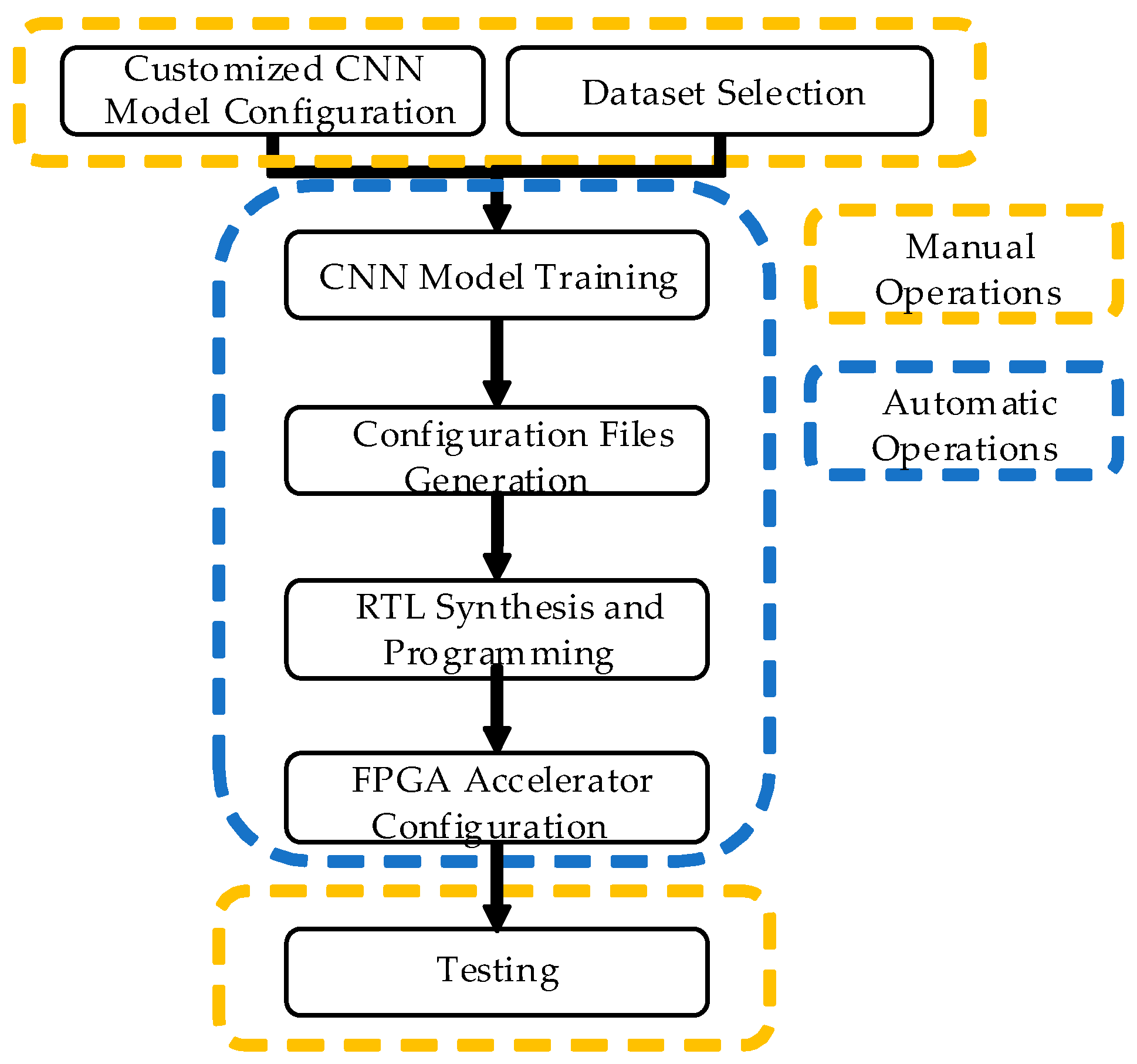
As shown in
Figure 1, the herein-presented platform allows the user to generate high-performance CNN accelerators by simply selecting the dataset and configuring the CNN model in a specialized graphical user interface (GUI) created for this specific purpose.
The platform uses third-party software to train the desired CNN model, as well as to synthesize RTL and program the FPGA device. Currently, the platform compatibility includes Tensorflow and MATLAB for training the CNN and Quartus II for synthesizing RTL and programming the FPGA device.
To allow the user to develop high-performance CNN models in FPGA in a straightforward manner, all hardware accelerators are built using configurable layers templates previously hand-coded in Verilog HDL. Currently, this platform contains convolutional, pooling, and fully connected layers and the ReLU and Softmax activation functions.
As CNN models become more accurate, their architectures are also becoming more complex; this complexity falls into two main categories: deeper architectures and the creation of new layers. Considering this, in addition to allowing the generation of customized CNN models, this template-based method makes it possible to include future layers in a straightforward manner for modern CNN models as they appear in the state-of-the-art.
To prove the functionality of the herein-presented platform, it was tested with some common CNN models for the freely available datasets MNIST [
16], CIFAR-10 [
17], and STL-10 [
18], as shown in
Table 1.
The main contributions of this work are as follows:
A proposal for a complete multi-system platform to generate CNN accelerators, from defining its structure to implementing a ready-to-use FPGA co-designed system in a few minutes;
An intuitive and easy-to-use GUI for generating customized CNN model accelerators for FPGA-based applications with user-selected image datasets;
An easily configurable CNN RTL template that can be upgraded for future CNN models.
The rest of this paper is organized as follows:
Section 2 presents a brief overview of the herein-presented platform.
Section 3 discusses the strategy followed to manage the data exchange between external and internal memory.
Section 4 contains the proposal for the CNN accelerator architecture.
Section 5 analyzes the results obtained from implementing customized CNN models with the herein-presented platform.
Section 6 presents the discussion.
2. Proposed Platform Overview
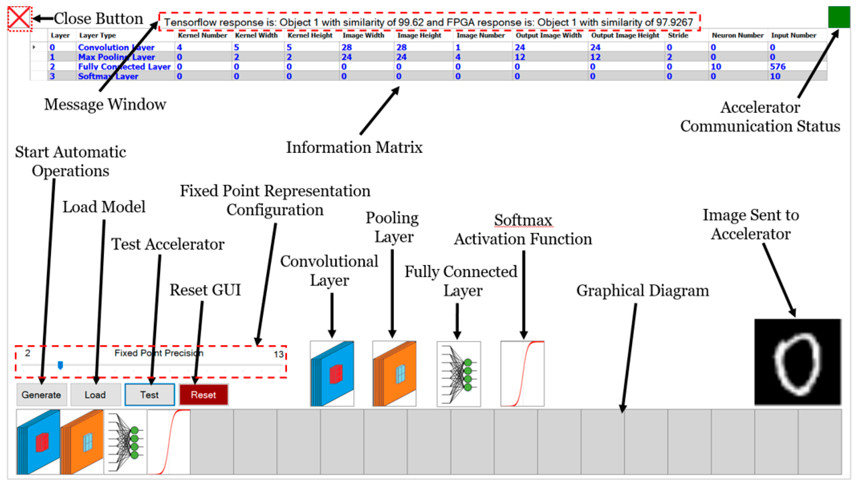
The entire process and every CNN accelerator are controlled with a PC-based specialized GUI system developed for this specific purpose, which can be used to generate a new CNN customized accelerator, load a previously created accelerator, and test the current accelerator. As shown in
Figure 1, the process for creating a customized CNN accelerator using the herein-presented platform consists of a specific sequence of manual and automatic tasks.
When creating a new accelerator for a customized CNN model, it is only required to configure sequence of layers and their internal parameters, including the selection of the desired dataset for training. Using the created CNN architecture and selected internal parameters, the platform generates an Information Matrix (InfM); such matrix is saved in a file, from which the CNN architecture is read when loaded with the platform. The InfM contains relevant details from the current CNN model, including the dataset and accuracy of the training, number of layers, order and type of layers, and parameters for every layer. For a deeper understanding of dataflow within the CNN, when adding layers, the InfM and the graphical diagram are refreshed at the top and bottom of the GUI, respectively, as shown in
Figure 2.
Then, a Tensorflow CNN model or MATLAB Deep CNN object is generated with corresponding parameters contained in the InfM and trained with the selected dataset. To use a custom dataset in MATLAB, it must be stored within a specific folder in the platform path, from where it can be loaded in the training and testing steps.
Once training is finished, the generation of the files required to create and configure the RTL starts. The first file is a top module HDL file (TMF); this Verilog file includes a series of parameter lists for generating the desired layers and hardware specifications. The external memory (DRAM) is not controlled by the layers, but rather by a Memory Arbiter (MemArb), which is completely independent from the layer execution schedule. This allows for the maximizing of off-chip memory throughput, as data is often available in on-chip buffers even before the layer is running. To achieve this, and taking advantage of the CNN iterative per-frame process, all memory accesses required to process an input image are scheduled prior to synthesizing the RTL. The off-chip memory-accessing schedule is stored in a file called Memory Commands File (MemComF), which is initialized in an on-chip BRAM to be accessed when managing off-chip memory accesses during execution. For MATLAB models, a Zerocenter Normalization Matrix file (NormF) is generated in case the user activates the input images normalization. The last file is the Weights File (WeightsF), containing the parameters from all convolutional layers filters and fully connected layers, which are stored in external DRAM during configuration stage.
When the abovementioned files are generated, the platform synthesizes the generated RTL using Quartus II and then programs the CNN accelerator in the physical Altera FPGA Board (DE2-115 for presented experiments). Once the CNN accelerator is programmed into the FPGA device, it is automatically configured through its communication sub-system (UART protocol). In this configuration process, some parameters are sent, and the weight values contained in WeightsF are stored in the off-chip DRAM memory.
At this point, the CNN accelerator is ready to be tested with the GUI. For testing the accelerator, the platform randomly selects and sends to the accelerator an image from the dataset. Then, the accelerator processes it and sends the results back to the GUI for displaying purposes.
3. Memory System
One of the main concerns when creating a high-performance digital system, especially for big-data applications, is reducing external memory accesses as much as possible, mainly because these accesses yield significantly more latency and energy consumption than on-chip memory accessing [
19]; therefore, internal data reusage must be prioritized.
3.1. External Memory
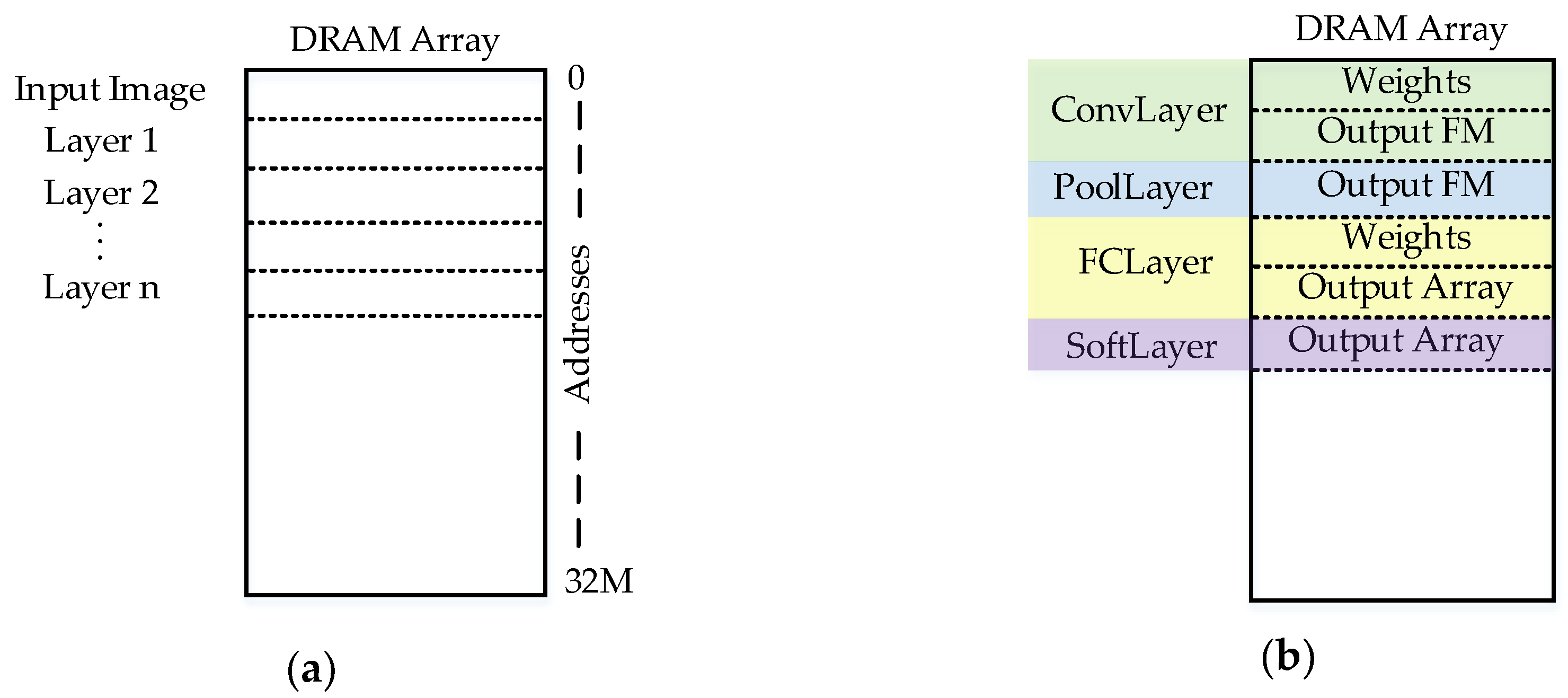
The main off-chip memory is a 32Mx32bit (128MB) DRAM used to store the input image, convolutional and fully connected layers weights, and output pixels of every layer. Due to on-chip memory limitations when using an FPGA device, all the layers share three configurable depth buffers, one writing buffer, and two reading (pixel [input] and weight) buffers. Every memory access is through the buffers, including the configuration process (when configuring FPGA accelerator).
As shown in
Figure 3, prior to configuring the CNN accelerator in the FPGA device, a section of the DRAM array is assigned to every layer with a fixed data arrangement (through MemComF).
All matrix-form data is stored row-by-row, matrix-by-matrix, taking advantage of burst-oriented DRAM behavior, allowing reading/writing with less latency (including input images, convolutional kernels, and feature maps). This arrangement also allows processing live camera streaming frames without modifications to the CNN accelerator architecture.
3.2. External Memory Accessing
The external memory (i.e., DRAM) is accessed with a customized hand-coded Verilog controller oriented to full-page burst reading/writing. This controller has been specially designed to improve accesses based on the DRAM memory arrangement shown in
Figure 3.
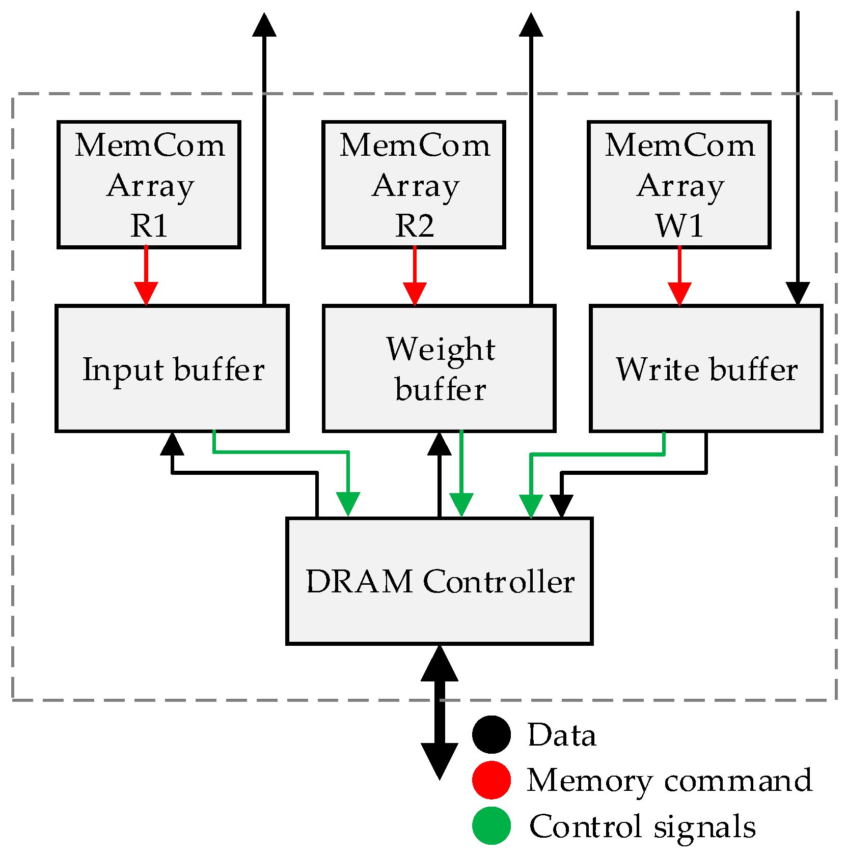
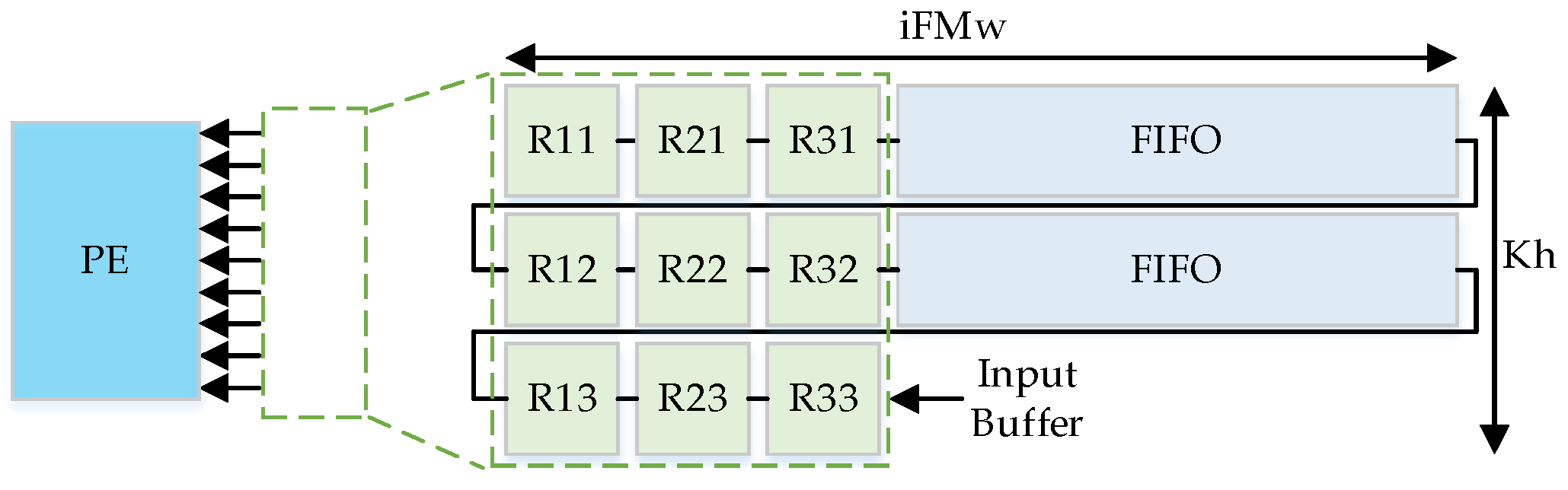
As can be seen in
Figure 4, the memory system contains two reading buffers and one writing buffer, each with a memory command array (MCA) containing the reading/writing patterns required to process an input image. The content of MemComF is stored in these arrays during RTL synthesis.
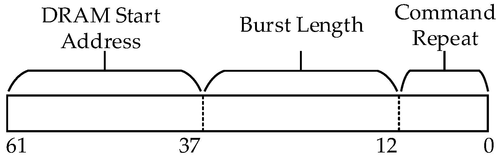
Thus, every DRAM access is requested by any buffer based on their memory schedule contained in MCA. Every Memory Command (MemCom) has the format shown in
Figure 5.
Each MemCom consists of three parameters; the 25 most significant bits correspond to the DRAM address where the first data is being read/written. Bits 36–12 represent the number of data to be read/written in the current burst access, and the 12 least significant bits determine the number of times that a command should be issued to the buffer. For example, to read an input color image of size 96 × 96, the CommandRepeat is 1, the Burst Length is 96 × 96 × 3 = 27,648, and the address is 0, resulting in a MemCom of 0x6C00001.
Each buffer has independent control, data, and address buses to the DRAM controller to avoid synchronization problems when more than one buffer requests access to the DRAM, and a hierarchical scheme is adopted where the writing buffer has priority over reading buffers.
To efficiently assign DRAM access to both reading buffers, there are two levels of urgency when they are nearly empty. These levels are 1% and 10% of available data from the maximum buffer capacity; nevertheless, these percentages are configurable. Using this approach, off-chip memory access is granted only when it is essential for preventing the reading buffers from emptying completely. If the input buffer is accessing the DRAM and the weight buffer reaches 1% of available data, the DRAM controller grants access to the weight buffer and vice versa.
4. Configurable CNN Accelerator
As mentioned in
Section 1, every CNN accelerator is built by instantiating hand-coded configurable Verilog layers with a template-based approach similar to that presented in [
9], and some hand-coded RTL blocks for a specific purpose, such as an external memory controller (i.e., DRAM) and a communication circuit (UART), among others.
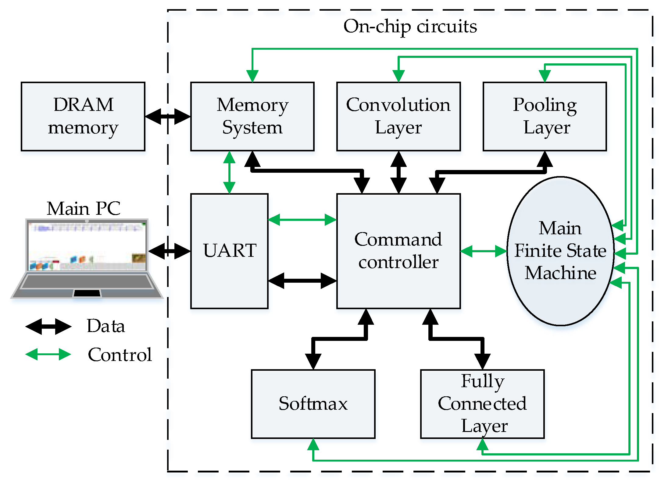
A top view of the CNN accelerator is shown in
Figure 6. This block-based architecture is generated by the top-level template (TMF), which is configured by the platform using the trained CNN model.
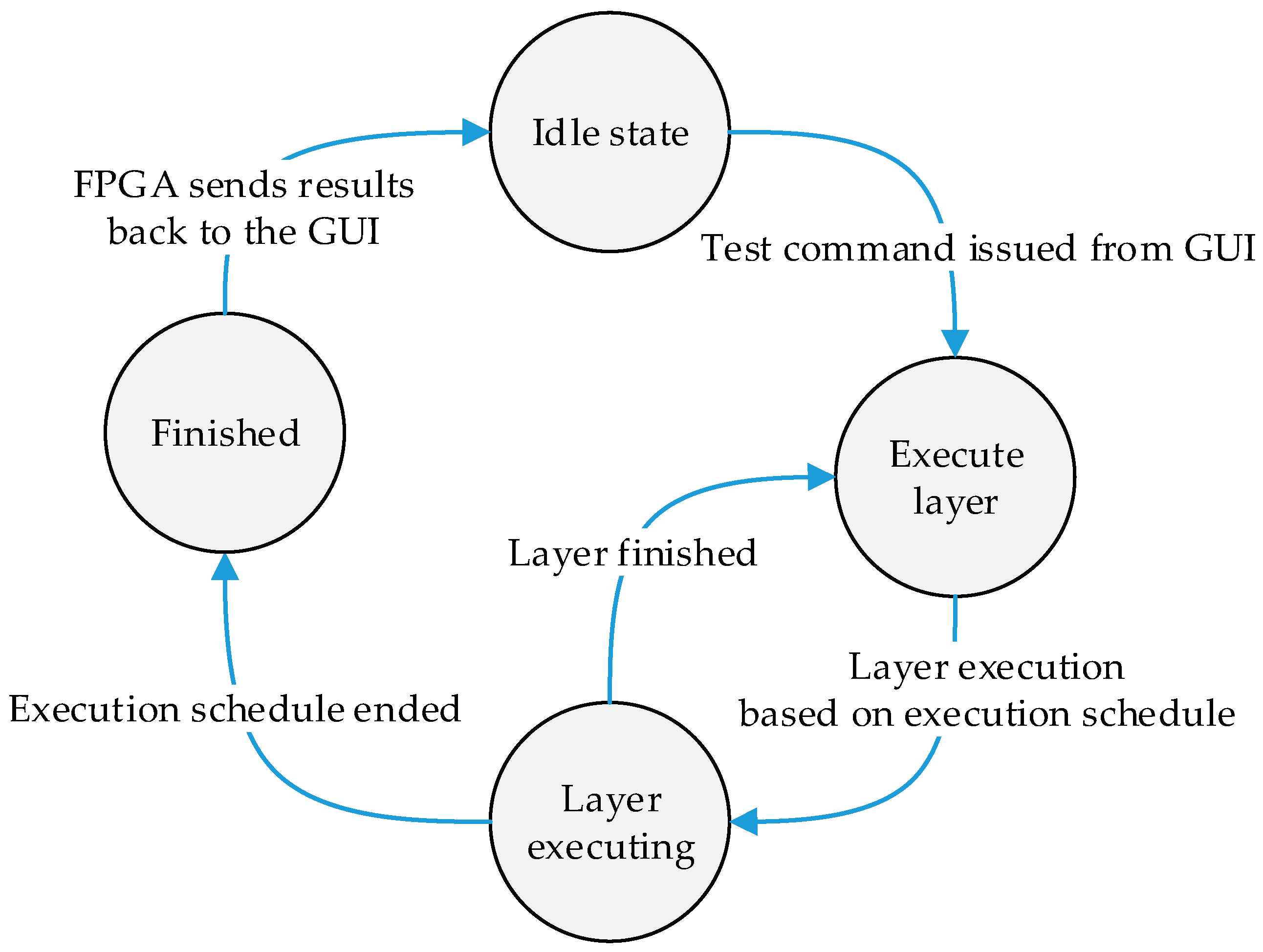
Layer-by-layer execution schedule is managed by the Main Finite Sate Machine (MainFSM), as shown in
Figure 7, which provides buffers access permissions to the layers and to the communication port (UART). The command controller’s main function is to decode commands coming from the MainPC and redirect data between memory system and all other circuits.
All layer templates are designed to be easily parametrizable for efficient hardware resource utilization to precisely fit the user-generated CNN model.
Figure 8 shows these configurable parameters of the hand-coded templates for the convolutional and pooling layer. Where iFMn, iFMw, and iFMh are the number, width, and height of input feature maps, respectively; kw, kh, and st are the kernel width, kernel height, and stride, respectively; and for the output feature maps, oFMn, oFMw, and oFMh are the number, width, and height, respectively.
All parameters shown in
Figure 8, with the exception of iFMn and oFMn, are assigned prior to synthesis; iFMn and oFMn are assigned during the configuration stage through the communication port (i.e., UART). Both layers share the same behavior and control; only the processing element (PE) is different.
4.1. Loop Unrolling Optimization
This section contains the loop optimization used in the herein-presented customizable CNN accelerator. By default, all convolutional layers implement this strategy. As noted above, all layers share three main buffers (i.e., input, weight, and writing buffers); this feature decreases control complexity, being this essential for creating a low-resource utilization system.
As can be seen in
Table 2, only Loop1 is unrolled, with factors of Pkw = Kw and Pkh = Kh. This strategy is adopted for two reasons: to prevent computation modules within PEs from entering to an unused state (i.e., when Pkw and Pkh are not divisible by Kw and Kh, respectively); this is also achieved by using unrolling factors of Pkw = Pkh = Pin = 1, as in [
9]. However, processing streaming frames becomes complex with this strategy, especially for the input convolution layer.
Additionally, PEs can be designed with a fully pipelined architecture, reducing writing buffer requirements, complexity, and the maximum frequency degradation of the system, at the cost of an increased number of external memory accesses.
4.2. Convolution Implementation Scheme
Kernel convolution operation is achieved with an internal data shifting scheme. As mentioned in
Section 3, all feature maps stored in external memory are arranged row-by-row, and therefore, the convolution dataflow adopts this behavior.
Convolution circuit is fully designed to compute input feature maps with streaming behavior by unrolling input feature map (see
Figure 9). This serves two purposes: to exploit the off-chip DRAM burst-oriented accessing and to enable live camera streaming processing, avoiding as much as possible storing input image in the off-chip DRAM.
This kernel window movement technique is employed in both convolution and pooling layers for increased hardware reusage.
4.3. Configurable Convolutional Layer
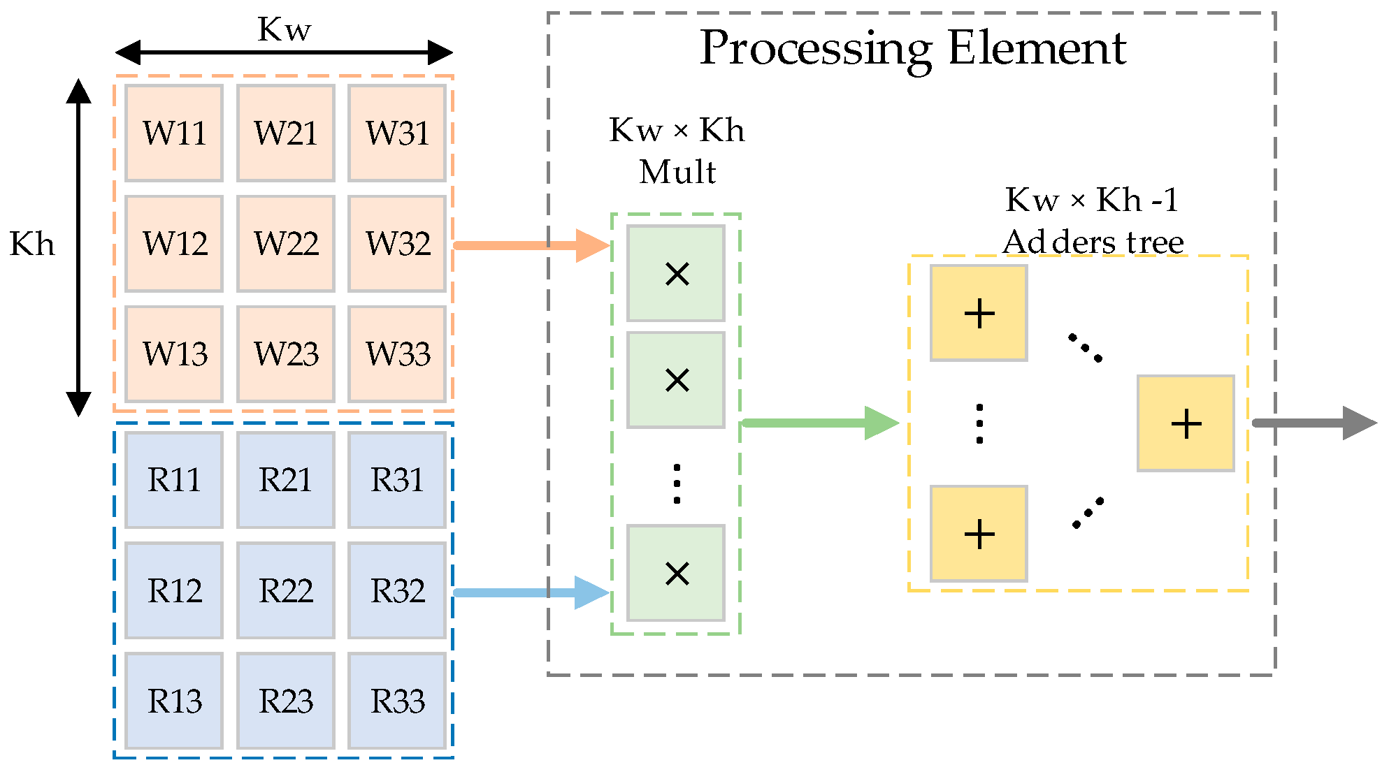
As mentioned in [
5], nearly 90% of total computations are carried out by convolutional layers (CL); this, and their parameter sharing schemes, makes them the most suitable layer for increasing acceleration and taking advantage of internal data reusage by using the massive parallel and pipelining capacity of FPGA devices.
Therefore, the design of an efficient PE is critical for obtaining a high-performance CNN accelerator; as noted above, Loop1 is fully unrolled, hence, the PE architecture is implemented as shown in
Figure 10.
Each convolutional layer uses a single PE with Kw × Kh parallel multipliers and a fully pipelined adders-tree with Kw × Kh -1 adders.
The CL process is designed in such a way that every final output pixel is calculated as fast as possible, using the unrolling factors shown in
Table 2. All final output feature maps are stored in off-chip memory (i.e., DRAM) to enable this platform to generate deeper CNN models with different input image sizes using the limited resources available in Cyclone IV EP4CEF29C7 FPGA [
20].
Once the MainFSM executes the CL, it begins to perform the calculations with the data contained in the on-chip pixel and weight buffers, according to its configuration. The CL reads Kw × Kh weights from the weight buffer and stores them in registers connected directly to its PE. Then, the first iFMw × iFMh input feature map is burst read from the pixel buffer and sent to the convolution circuit shown in
Figure 9. The partial oFMw × oFMh output feature map is stored completely in on-chip memory using a multiply–accumulate (MAC) operation to reduce external memory accesses. This process is repeated iFMn × oFMn times, and every iFMn iterations of the final output image is passed through the ReLU function in case it has been activated. The ReLU function is implemented using a multiplexer with the sign bit as selector, and then the resulting final output feature map is stored in external DRAM memory. When this process is complete, the CL asserts a flag connected to the MainFSM, to continue layer execution schedule.
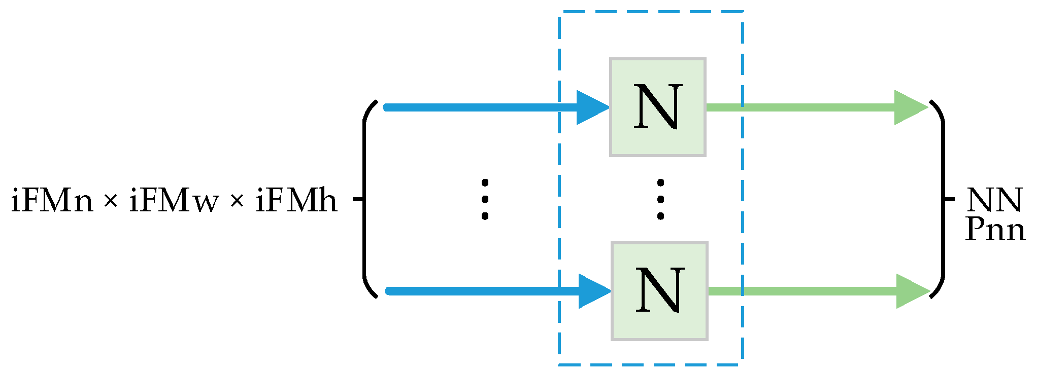
4.4. Configurable Pooling Layer
When the MainFSM executes pooling layer (PL), PL sequentially reads iFMn × iFMw × iFMh pixels from the pixel buffer, streaming them to the convolution circuit shown in
Figure 9 with the corresponding configured sizes. As seen in
Figure 11, PL processing element consists of a fully pipelined comparator tree with Kw × Kh – 1 comparator modules with a fan-in of Kw × Kh.
4.5. Configurable Fully Connected Layer
Unlike convolutional layers, in conventional CNN models, fully connected layers (FCL), also called dense layers, represent a low percentage of total computations. In contrast, most CNN weights are required for computing FCL function because they do not have the convolutional layer’s weight-sharing property. Additionally, in FCL, two values are required for processing every input pixel: the pixel value itself and a weight value.
These requirements speak to the main problem for designing an efficient FCL hardware accelerator: memory accessing. Additionally, on-chip memory blocks in FPGA devices are very limited, so FCL weight values must be stored in external memory, which implies slower computations. This issue can be attenuated by reusing input pixels by parallelizing neuron nodes computation.
The FCL template is configured by assigning the parameters shown in
Figure 12, where iFMn, iFMw, and iFMh are the number, width, and height of the input feature maps, respectively; NN is the number of neurons; and Pnn is the number of parallel neuron nodes implemented in hardware, which is always a divisor of NN for efficient hardware reusage within FCL.
Every neuron node is implemented using one MAC unit with shared input pixel, which is multiplied by different Pnn weight values. ReLU activation function is applied in case it has been activated.
By parallelizing computations implementing Pnn neuron nodes, Pnn weight values must be read for every calculation. Since both CNN accelerator and external DRAM memory work at the same frequency and only one weight buffer is used, it was assigned Pnn = 1 for the experiments, because parallel computing cannot be efficiently achieved. However, our configurable accelerator is designed to implement parallel neuron nodes in case of a faster external memory is used (i.e., DDR). To overcome this, all input pixels for computing FCL are stored in on-chip BRAM, so that external memory throughput can be fully available for weight burst reading.
4.6. Numeric Representation
As mentioned in
Section 1, the herein-presented generator is compatible with Tensorflow and MATLAB deep learning frameworks. Since trainable parameters and feature maps values depend on the used framework and trained CNN architecture, a single numeric representation is not suitable for a configurable CNN accelerator. Therefore, this platform is able to generate accelerators with 16 and 32 bits architectures; for 16-bit architectures, numeric representation (number of integer and fractional bits) can be configured during run-time or prior to synthesis. For deeper networks, the number of integer bits must be increased in order to prevent overflow.
4.7. Softmax Activation Function
The Softmax activation function (SAF) is optionally applied to the last FCL in CNN models in order to normalize neuron node outputs to values within the range (0,1) with Equation (1)
where
NN is the number of neuron nodes in FCL,
y(
n) is the output of softmax function, and
xn is the output of the neuron node.
As shown in Equation (1), the output of SAF depends on the nonlinear exponential function, so a fixed-point representation is not adequate for such operations.
To obtain accurate results implementing SAF, a single-precision floating-point representation is used, based on standard IEEE 754-2008 [
21]. As previously mentioned, FCL uses fixed-point arithmetic; thus, a conversion stage is required from a fixed-point to a single-precision floating-point, which processes all SAF inputs before performing required operations.
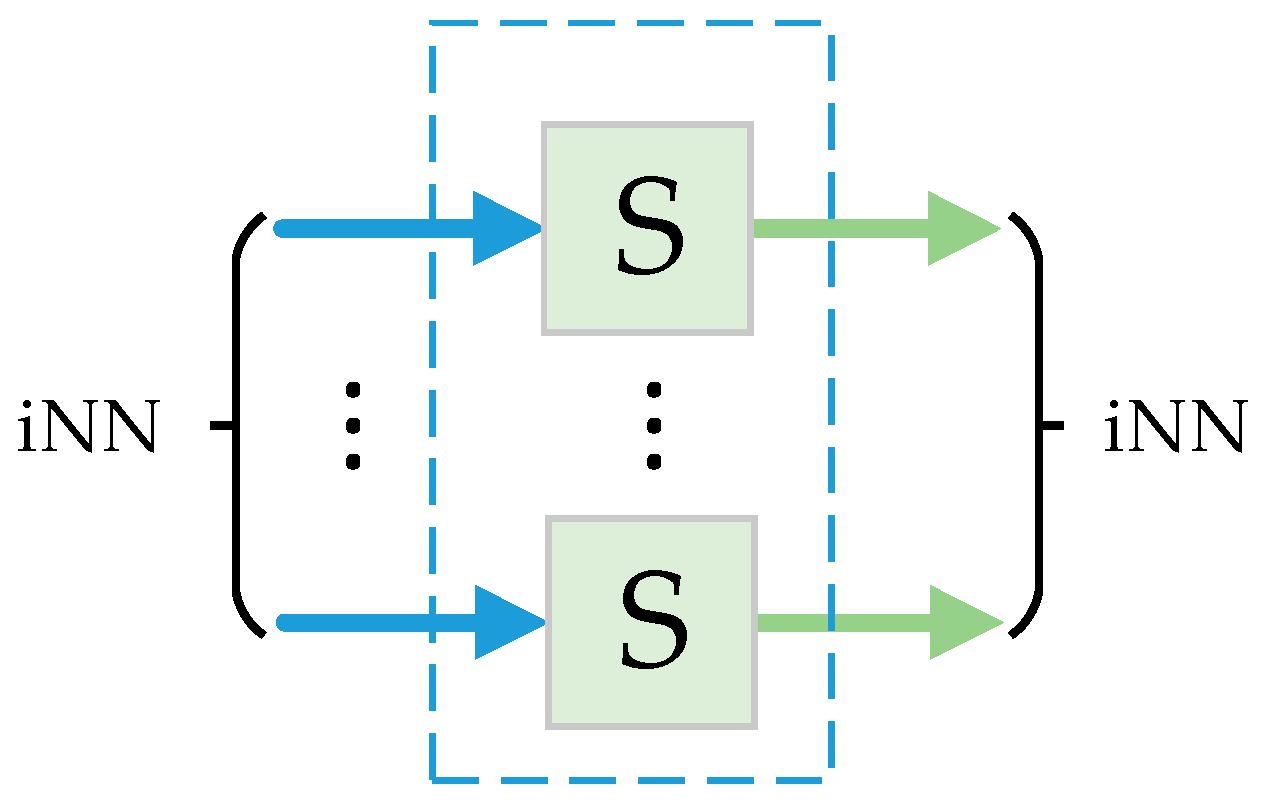
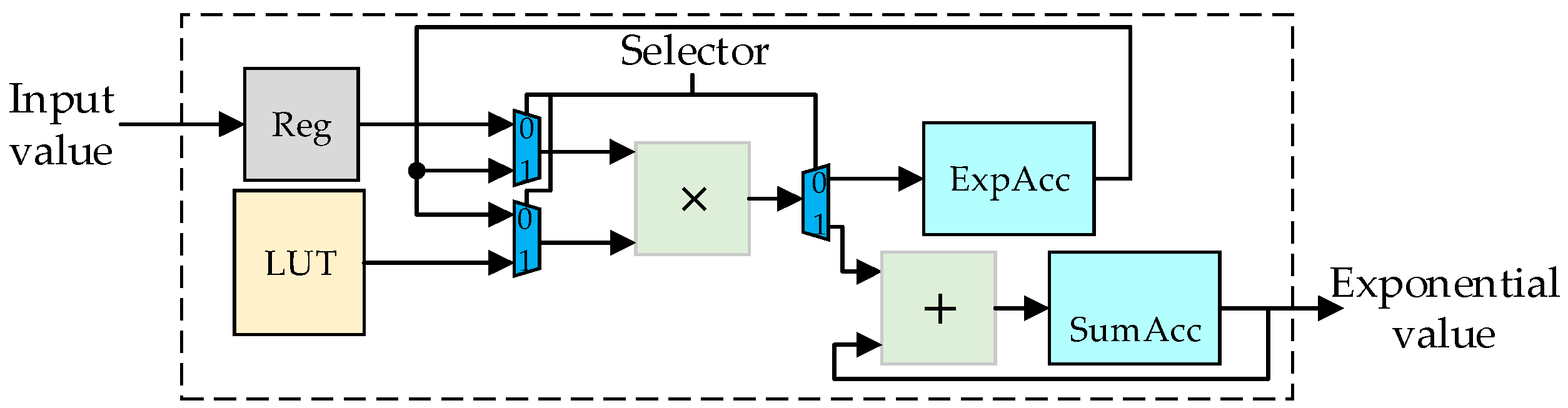
Due to its complexity, the control of the activation function is simplified by managing the SAF as an independent layer using the architecture shown in
Figure 13, where iNN is the number of neuron nodes in previous FCL. Therefore, it is also executed with the MainFSM execution schedule.
When SAF is executed, it reads one data from pixel buffer, which is directly sent to the conversion stage. Once the data is in single-precision format, it is redirected to an exponential calculator. The exponential value is stored in an on-chip memory (with iNN locations) in the SAF and added to an accumulator. This process is repeated iNN times; when the iterations are finished, the divisor from (1) is extracted from the accumulator.
To obtain the result of every SAF output, the exponential values stored in on-chip memory in the previous loop are divided by the content of the accumulator. Since division is one of the operations that are critical from the point of view of hardware implementation, it was implemented using repeated subtraction method. This methodology carries more latency (around 40 clock cycles per division); nevertheless, this operation is performed few times per image processed.
This process is repeated iNN times, and in every iteration, the division result is sent to the writing buffer. The exponential function is implemented using Taylor series approximation shown in Equation (2), with a configurable number of iterations (
Tn); Tn is set from 15 to 25 in the experiments.
As can be seen in Equation (2), the divisor of the summation is the factorial of the iteration number. It is not run-time calculated, but the reciprocals from Tn factorial consecutive numbers are stored in a lookup table, from which the values are read during execution; this strategy allows obtaining exponential results more quickly, because no division is required.
With this approximation, the exponential is calculated by a simple loop with Tn iterations.
Figure 14 shows the block diagram of the exponential calculator; when the selector is set to zero, the logic is used to calculate the dividend of the summation shown in Equation (2); otherwise, logic is used to calculate and accumulate the partial output.
5. Experimental Results
The main purpose of the proposed platform is to generate CNN accelerators from custom and conventional CNN models automatically using highly configurable hardware templates, which is demonstrated by generating some low-end conventional and custom CNNs models for freely available datasets, such as, MNIST, CIFAR-10, and STL-10.
The platform was tested on a PC with HDD, i5-8300H CPU @ 2.3 GHz, 8 GB DRAM @2667 MHz, and a 4 GB Nvidia 1050 GPU. All experiments were performed using an Intel Cyclone IV FPGA (Intel, San Jose, CA, USA), with a total of 115K logic elements (LEs), 532 embedded 9-bit multipliers, and 3.8 Mbits of embedded on-chip memory. The Intel Cyclone IV FPGA (Intel, San Jose, CA, USA) device is embedded in the DE2-115 Terasic (Terasic, Hsin Chu, Taiwan) board, with a 50 MHz clock source, and two SDRAM memories connected in parallel with a total of 128 MB and a 32-bit bus width.
All internal FPGA data is represented using fixed-point format, with the exception of SAF (optionally included), which uses a single-precision floating-point representation based on standard IEEE 754-2008 [
21]. Every CNN accelerator uses a phase-locked loop (PLL) configured according to the maximum circuit frequency. Models with softmax activation function work at a frequency of 75 MHz; otherwise, their PLL is configured at 100 MHz.
5.1. 32-Bit Architecture
For 32-bit architecture, experiments were carried out by generating five different CNN models with MATLAB. Two small conventional CNNs (i.e., LeNet5 [
1] and CFF [
22]), and three custom CNN models called Model1, Model2, and Model3), trained with MNIST, CIFAR-10, and STL-10 datasets, respectively, were used, whose architectures are shown in
Table 3 (ReLU function is not shown for the sake of brevity).
As can be seen in
Table 4, for 32-bit architectures, a fully functional CNN accelerator can be designed and tested on-board in few minutes using the presented platform, where Model1 has the shortest generation time with 00:03:54 and, as shown in
Table 5, Model1 also carries the lowest hardware requirements and latency, because of its simplicity and the low number of parameters. In contrast, Model3 is the deepest architecture, whose generation time is 00:42:27, due to the complexity of its architecture and the input image size in comparison to low-end CNN models (e.g., LeNet-5 and CFF). Analyzing
Table 4, approximately 60% of time required to generate a Model3 CNN accelerator is consumed by two processes. The most time-consuming process is FPGA configuration, where all weights and configuration parameters are stored in DRAM and registers, representing approximately 33% of the total time; however, this time is decreased by using 16-bit architectures.
5.2. 16-Bit Architecture
Many signal processing applications are best suited for fixed-point 16 bits architecture [
23]. Using this representation, five CNN models were generated using Tensorflow framework, including two small conventional CNNs (i.e., LeNet-5 [
1] and CIFAR [
24]) and three custom CNN models called Model4, Model5, and Model6, trained with MNIST, CIFAR-10, and STL-10 datasets, respectively, whose architectures are shown in
Table 6.
As shown in
Table 7, using 16-bit architecture, generation time is reduced in some tasks (i.e., configuration files and FPGA configuration) with respect to
Table 4 (32-bit architecture), due to the lower bit representation.
As can be seen in
Table 8, for 16-bit architecture implementations, latency is reduced approximately by a half with respect to 32-bit architecture (
Table 5) but resources requirement is not decreased because higher parallelization is applied. On the other hand, on-chip memory requirement is reduced due to the fewer bits required to store partial oFM in convolutional layers and shortest FIFO memory for convolution operation.
5.3. Experiments Analysis
The graphs in
Figure 15 show the percentage of the latency/image consumed by each type of layer for the custom models generated in the experiments. Due to the number of filters in each CL, the low parallelization levels applied in Model3, and the fixed unrolling factors, the convolutional layers consume the most time for the processing of an input image. On the other hand, for Model1 and Model4, FcL requires almost half of the latency due to external memory throughput, due to the fact that a single neuron node is generated (
Pnn = 1).
FPGA configuration process is slow for 32-bit architectures; this can be attributed to the relatively low speed communication port (UART), which works at a baud rate of 115200 bps. This could be improved by using a faster communication protocol (e.g., USB and PCI-EXPRESS), as in [
10], where a configuration time of approximately 366 ms to configure VGG model using PCI-EXPRESS is reported.
The generation of configuration files takes approximately 27% for Model3 (32-bit) and 4% for Model6 (16-bit) of total time; such files allow our tool to implement previously trained CNN models.
Table 5 and
Table 8 shows the performance of the hardware accelerators implemented using the proposed tool. Resources utilization depends greatly on CLs filter sizes, due to the applied unrolling optimization factors.
Model2 accelerator requires approximately 10% more resources than Model3, despite Model3 being deeper. This is because CL kernels are larger, so by fully unrolling Loop1, more parallel multipliers and bigger adders-trees are required, but the frame processing time is reduced.
Model3 is the deepest CNN model implemented in the experiments. It was trained to classify STL-10 dataset, which consist of 10 classes of 96x96 color images. Its architecture is based on that proposed in [
25] for the CIFAR-10 dataset, with some modifications. The usage of on-chip memory resources overwhelmed the requirements in other models due to the size of the input image, mainly because partial oFM of CL are fully stored in on-chip memory for faster computation.
Latency in Model3 is high in comparison with other CNN models implemented in experiments. This is because only Loop1 is unrolled. As it is a Kw = Kh = 3 loop (relatively small), low parallelization levels are applied; this is verified by the low hardware resources utilization with Model3.
6. Discussion
The herein-presented co-designed HW/SW system aims to reduce the gap between CNN models and its fast prototyping in FPGA devices. This is achieved by proposing a system-flow to generate FPGA-based accelerators from fully customized CNN models in minutes.
Additionally, users can generate many FPGA-based CNN models without requiring in-depth knowledge of CNN algorithm and hardware development techniques, because the process to train, generate, and configure CNN accelerators is fully automated.
The used template-based scheme allows one to integrate new layers for modern CNN models and add features to the existing layers with ease. All RTL blocks are hand-coded Verilog templates; thus, our tool can be modified to use FPGAs from different vendors (e.g., Xilinx), by changing the external memory controller (if necessary). As no IP is used, every CNN accelerator can be processed to develop an ASIC in a straightforward manner; such methodology has yielded good performance, as demonstrated in [
26], for low bit-width convolutional neural network inference.
Currently, this platform uses Tensorflow and MATLAB to train CNN models; nevertheless, we are working on adding support for other freely-available deep learning frameworks, e.g., Caffe, giving our platform the capacity to generate custom CNN accelerators with most used frameworks.
In order to obtain a more robust platform, layers templates will be improved by adding the capacity to infer quantized and pruned convolutional neural networks, reducing drastically the number of operations and memory required for benchmark CNNs (e.g., AlexNet), as explained in [
27].
To enhance the throughput of CNN models with small kernel sizes (e.g., Model3), and to exploit massive FPGA parallelism, we will improve our Verilog templates by introducing unrolling and tiling factors as configuration parameters based on the work in [
7].


