Open-Circuit Fault Analysis and Modeling for Power Converter Based on Single Arm Model

Abstract

This paper proposes a new modeling method for power converter based on single arm model. The objective of this paper is twofold: (1) One is to present the single arm model with good portability. The single arm model can be used to build the models of power converters which have several arms with the same structure; (2) the other is that the converter model built by the single arm model can represent the power converter when open-circuit faults happened in power devices and clamping diodes. First of all, the inputs and outputs of single arm are redefined. Then, the open-circuit faults occurring in different power devices and clamping diodes are analyzed. Furthermore the single arm model is built. Finally, the model of power converter is established based on the single arm model, which can express the power converter with open-circuit fault. The effectiveness and accuracy of the proposed model have been verified by simulation and experiment results.

1. Introduction

Power converters are found in a vast number of applications, such as renewable energy conversion systems, power grids and high-speed trains [1,2,3]. Usually, the power devices of a converter are in a long-term state of high frequency modulation and bear high voltage and large current with relatively serious heating and large switching losses [4]. In addition, power converters often require uninterrupted operation. Such harsh work conditions may cause a series of problems, like parameter drift and component damage, which would eventually lead to deterioration of power devices performance. It is reported that about 38% of the faults in power converters are caused by the power devices faults [5]. The power devices faults mainly include open-circuit faults and short faults [6,7,8]. When a short fault occurs, the power device will be burned out at a very limited duration and the short fault will turn to open-circuit fault finally [9]. When an open-circuit fault occurs in a power device, the adjacent power devices will bear larger current and higher voltage. If the open-circuit fault can not be dealt with in time, the secondary fault will be triggered easily [10].

Hence, the diagnosis and tolerance of open-circuit faults have become hot topics in the past few decades, but there is a lack of open-circuit fault data, especially in high power fields, such as high-speed trains and power grids. Physical experiment is a way to get open-circuit fault data but it is usually costly and dangerous. The hardware-in-the-loop simulation is more reliable than the off-line simulation and has become an important way to obtain data [11,12,13], but a mathematical model which can represent the power converter with open-circuit faults is needed for the hardware-in-the-loop (HIL) simulation. So the modeling method of open-circuit faults has become an important problem to be solved.

There are two common types of modeling methods for the power converter, the switching function-based method and the controlled source-based method. In the former one, the arms of power converters are simplified as switching functions [14,15,16,17]. Different kinds of command signals correspond to different switching function values. Then, the model of rectifier or inverter is built as a whole. It is suitable to build the power converter models whose command signals are not very complicated, such as two-level and three-level converters in the normal condition. When open-circuit faults occur, the complexity of command signals increases sharply. Like the three-level converter, there are three kinds of command signals for one arm in the normal condition; when open-circuit faults occur in power devices, there are seven kinds. If open-circuit faults in clamping diodes are also considered, there will be thirteen kinds of operation modes for a single arm, such that the switching function-based method is inapplicable for the open-circuit fault modeling. In the latter one, the converter is equivalent to a controlled source which can be divided into state-space averaging method and dq-domain method [18,19,20]. The major purpose of establishing power converter model by controlled source-based method is the stability analysis of the system. Unfortunately, the inner details of every power device are unfeasible, which leads to difficulty in building the open-circuit fault models. Most of the existing models can only express the power converter in normal condition. The attention focusing on modeling of power converters with open-circuit faults is rare. Recently, a fault-injection platform has been developed in [21] and used for validation of various fault detection methods in [22,23]; it is not a mathematical model, but a circuit model. According to circuit topology, the fault-injection platform is established by commercial encapsulated modules. Note that it is an off-line simulation platform, which can be used for faults testing, but cannot be applied for hardware-in-the-loop simulation and validating the real-time of open-circuit fault detection, diagnosis and tolerance methods. A uniform modeling method is present in [24], but there is not a model which can represent the power converter with an open-circuit fault in clamping diodes. To the best of our knowledge, there is a lack of work about modeling of power converters which can express the converter with open-circuit faults in any power device and clamping diode.

Motivated by the above discussions, a modeling method for power converters based on single arm model is proposed in this paper. To build the model of a power converter, first of all, the inputs and outputs are redefined. After that, the relationship of the inputs and outputs of the single arm are analyzed in open-circuit fault cases. Subsequently, the single arm model is established, which can represent the single arm with open-circuit faults. Finally, combining the circuit topology and the proposed model, the complete model of power converter is built.

There are two main advantages of the modeling method. One is the portability, which has two meanings. First, no matter how many power devices and clamping diodes in the power converter, the model can be established by this method. To be specific, the method can not only build the two and three level converter, but also five and even-higher-levels converters. Second, only a single arm needs to be analyzed instead of the whole power converter in the modeling process. Once the single arm model is established, it can represent all arms with the same structure, so it is the method suitable to build the models of power converters which have several identical arms. The other is the uniformity, the model established by the proposed method can represent the converter not only in normal conditions but also abnormal conditions that open-circuit faults occur in any power devices and clamping diodes. Besides, the model established by the proposed method can be used for real-time simulation. The model can be used for the hardware-in-the-loop simulation and provide a more reliable platform and data source for open-circuit fault detection, diagnosis and tolerance.

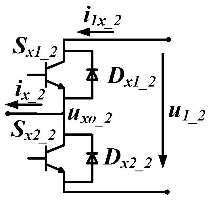
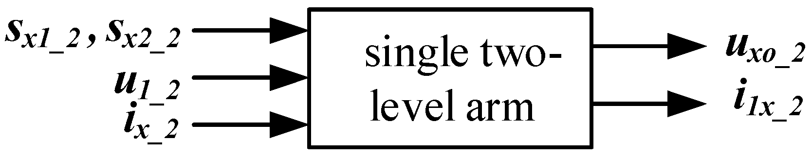
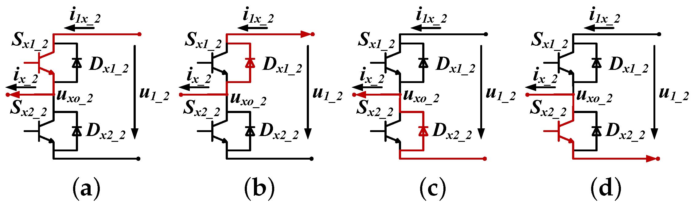
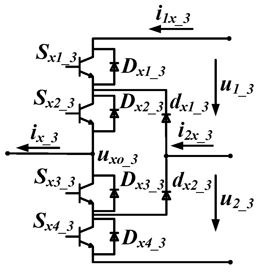
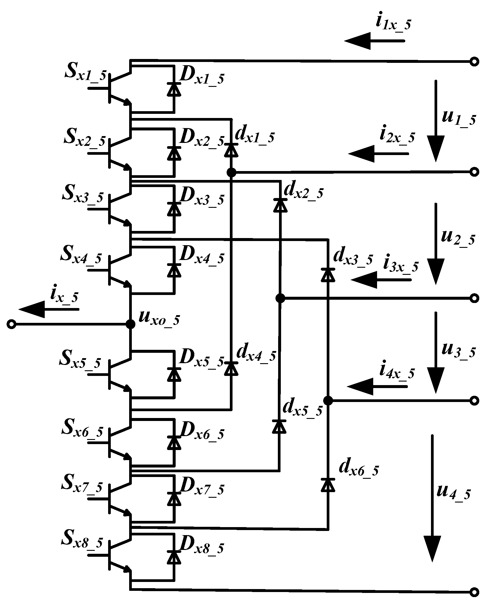
The type of AC–DC–AC converter is chosen to explain the modeling method in detail. The modeling processes of three kinds of single arms are given, which are commonly used in power converters and a general formula is given in Section 2. Then, the general model of AC–DC–AC converter is built based on the single arm model, which is given in Section 3. The model can represent the converter when open-circuit fault occurs. In order to verify the effectiveness and accuracy of the model and modeling method proposed, two testing platforms of three-level converters are established, the simulation and experiment results are shown in Section 4. The conclusions are given in Section 5.

2. Open-Circuit Fault Analysis and Single Arm Model

Practical power converters usually include several arms with the same structure, such as AC –DC–AC converter, which includes rectifier, DC-link and inverter. The rectifier and inverter consist of several identical arms, the DC-link is made up of several support capacitances [25,26,27]. The rectifier is connected to the power grid, which translates AC into DC. The inverter is connected to the loads, which converts DC to AC. The DC-link is used to absorb the power difference between the rectifier and the inverter and makes the system more stable. The major functions of the converter are realized by the rectifier and inverter, and the major functional units of the rectifier and inverter are the arms. If the single arm model is established, the converter model will be built easily. Then, three kind of single arm models are built, which are commonly used in AC–DC–AC converters. The general formula of single arm model is given at the end.

2.1. Single Two-Level Arm Model

The topology of a single two-level arm is shown in Figure 1. $S_{x1\_2}$ and $S_{x2\_2}$ are the power devices in the $xth$ ($x=1,2\dots m_2$) arm, the command signals of them are $s_{x1\_2}$ and $s_{x2\_2}$. $D_{x1\_2}$ and $D_{x2\_2}$ are the freewheel diodes. $i_{x\_2}$ and $u_{xo\_2}$ are the phase current and phase voltage of the $xth$ arm, respectively. $i_{1x\_2}$ is the current from the DC-link to the $xth$ arm. $u_{1\_2}$ is the voltage of the capacitance in the DC-link. In order to build the single two-level arm model conveniently, the inputs and outputs of single two-level arms are redefined and shown in Figure 2.

For each arm, there is no more than one command signal that is high at the same time. If there is no command signal that is high, there is a dead-time period or an open-circuit fault occurring in a power device. The power devices often experience open-circuit faults in applications. When an open-circuit fault is occurring in power devices, the relationship between the inputs and outputs of a single three-level arm will be changed. Analysis of the normal condition and open-circuit faults are given in the following.

In the normal condition, there are two kinds of command signals for a single two-level arm, that are 10 and 01. Whether the phase current $i_{x\_2}$ is negative or positive, the relationship between the inputs and outputs of a single three-level arm is not changed. When the command signal is 10, if $i_{x\_2}$ is positive, it flows through $S_{x1\_2}$, as shown in Figure 3a, if $i_{x\_2}$ is negative, it flows through $D_{x1\_2}$, as shown in Figure 3b. On these occasions, $u_{xo\_2}=u_{1\_2}/2$ and $i_{1x\_2}=i_{x\_2}$. When the command signal is 01, if $i_{x\_2}$ is positive, it flows through $D_{x2\_2}$, as shown in Figure 3c; if $i_{x\_2}$ is negative, it flows through $S_{x2\_2}$, as shown in Figure 3d. On these occasions, $u_{xo\_2}=-u_{1\_2}/2$ and $i_{1x\_2}=0$.

When an open-circuit fault occurs in a single two-level arm, there will be a new kind of command signal; it is 00. If $i_{x\_2}$ is positive, it flows through $D_{x2\_2}$, as shown in Figure 3c. On this occasion, $u_{xo\_2}=-u_{1\_2}/2$ and $i_{1x\_2}=0$. If $i_{x\_2}$ is negative, it flows through $D_{x1\_2}$, as shown in Figure 3b. On this occasion, $u_{xo\_2}=u_{1\_2}/2$ and $i_{1x\_2}=i_{x\_2}$.

By the analysis above, the relationship between the inputs and outputs of a single three-level arm in different command signals is given in

Table 1. Relationship between inputs and outputs of a single two-level arm.

Condition	Command Signals	${\mathit{i}}_{\mathit{x}\_2}$	${\mathit{u}}_{\mathit{xo}\_2}$	${\mathit{i}}_{1\mathit{x}\_2}$
Normal	10	$i_{x\_2}\ge 0$	$u_{1\_2}/2$	$i_{x\_2}$
	01		$-u_{1\_2}/2$	0
	10	$i_{x\_2}<0$	$u_{1\_2}/2$	$i_{x\_2}$
	01		$-u_{1\_2}/2$	0
Faults	00	$i_{x\_2}\ge 0$	$-u_{1\_2}/2$	0
	00	$i_{x\_2}<0$	$u_{1\_2}/2$	$i_{x\_2}$

.

Combining the analysis of a single two-level arm and Table 1, the single two-level arm model is obtained by the following equation:

$$\left\{\begin{array}{c}{u}_{xo\_2}=\frac{[c_{x\_2}(s_{x1\_2}-s_{x\overline{1}\_2})+c_{\overline{x}\_2}(s_{x\overline{2}\_2}-s_{x2\_2})]u_{1\_2}}{2}\hfill \\ i_{1x\_2}=(c_{x\_2}{s}_{x1\_2}+c_{\overline{x}\_2}{s}_{x\overline{2}\_2})i_{x\_2}\hfill \end{array}\right.$$

(1)

where $x=1,2\dots m_2$, stands for the first, second... the $m_{2}th$ arm, respectively. $c_{x\_2}$ is the flag of $i_{x\_2}$, if $i_{x\_2}\ge 0$, $c_{x\_2}=1$, $c_{\overline{x}\_2}=0$; if $i_{x\_2}<0$, $c_{x\_2}=0$, $c_{\overline{x}\_2}=1$.

2.2. Single Three-Level Arm Model

The topology of a single three-level arm is shown in Figure 4. $S_{x1\_3}$, $S_{x2\_3}$, $S_{x3\_3}$, and $S_{x4\_3}$ are the power devices in the $xth$ ($x=1,2\dots m_3$) arm, the command signals of them are $s_{x1\_3}$, $s_{x2\_3}$, $s_{x3\_3}$, and $s_{x4\_3}$. $D_{x1\_3}$, $D_{x2\_3}$, $D_{x3\_3}$, and $D_{x4\_3}$ are the freewheel diodes. $d_{x1\_3}$ and $d_{x2\_3}$ are the clamping diodes. $q_{x1\_3}$ and $q_{x2\_3}$ are the flags of them. The values of $q_{x1\_3}$ and $q_{x2\_3}$ are 1 stands for clamping diodes operating in the normal condition. The value of $q_{x1\_3}$ or $q_{x2\_3}$ turning to 0 means an open-circuit fault happened in $d_{x1\_3}$ or $d_{x2\_3}$. $i_{x\_3}$ and $u_{xo\_3}$ are the phase current and phase voltage of the $xth$ arm, respectively. $i_{1x\_3}$ and $i_{2x\_3}$ are the currents from the DC-link to the $xth$ arm. $u_{1\_3}$ and $u_{1\_3}$ are voltages of the capacitances in the DC-link. Like the single two-level arm, the inputs of the single three-level arm are command signals, the voltages of the DC-link and the phase current. The outputs of the single three-level arm are the phase voltage and the currents from the DC-link to the $xth$ arm.

In the normal condition, there are three kinds of command signals for a single three-level arm; they are 1100, 0110 and 0011. $q_{x1\_3}$ and $q_{x2\_3}$ are 11. When the command signal is 1100, if $i_{x\_3}$ is positive, current paths are as shown in Figure 5a; if $i_{x\_3}$ is negative, current paths are as shown in Figure 5b. $u_{xo\_3}=u_{1\_3}$, $i_{1x\_3}=i_{x\_3}$, and $i_{2x\_3}=0$. When the command signal is 0110, if $i_{x\_3}$ is positive, current paths are as shown in Figure 5c; if $i_{x\_3}$ is negative, current paths are as shown in Figure 5d. $u_{xo\_3}=0$, $i_{1x\_3}=0$, and $i_{2x\_3}=i_{x\_3}$. When the command signal is 0011, if $i_{x\_3}$ is positive, current paths are as shown in Figure 5e; if $i_{x\_3}$ is negative, current paths are as shown in Figure 5f. $u_{xo\_3}=-u_{2\_3}$, $i_{1x\_3}=0$, and $i_{2x\_3}=0$.

When an open-circuit fault happened in clamping diodes, the current paths will be influenced while command signal is 0110. If $i_{x\_3}\ge 0$, the open-circuit fault occurs in $d_{x1\_3}$ and the current paths are as shown in Figure 5e. $u_{xo\_3}=-u_{2\_3}$, $i_{1x\_3}=0$, and $i_{2x\_3}=0$. If $i_{x\_3}<0$, the open-circuit fault occurs in $d_{x2\_3}$ and the current paths are as shown in Figure 5b. $u_{xo\_3}=u_{1\_3}$, $i_{1x\_3}=i_{x\_3}$, and $i_{2x\_3}=0$.

When an open-circuit fault occurs in power devices, there will be four new kinds of command signals; they are 1000, 0100, 0010 and 0001. When the command signal is 1000, if $i_{x\_3}\ge 0$, the current paths are as shown in Figure 5e. $u_{xo\_3}=-u_{2\_3}$, $i_{1x\_3}=0$, and $i_{2x\_3}=0$. If $i_{x\_3}<0$, the current paths are as shown in Figure 5b. $u_{xo\_3}=u_{1\_3}$, $i_{1x\_3}=i_{x\_3}$, and $i_{2x\_3}=0$. When the command signal is 0100, if $i_{x\_3}\ge 0$, current paths are as shown in Figure 5c. $u_{xo\_3}=0$, $i_{1x\_3}=0$, and $i_{2x\_3}=i_{x\_3}$. If $i_{x\_3}<0$, current paths are as shown in Figure 5b. $u_{xo\_3}=u_{1\_3}$, $i_{1x\_3}=i_{x\_3}$, and $i_{2x\_3}=0$. When the command signal is 0010, if $i_{x\_3}\ge 0$, current paths are as shown in Figure 5e. $u_{xo\_3}=-u_{2\_3}$, $i_{1x\_3}=0$, and $i_{2x\_3}=0$. if $i_{x\_3}<0$, current paths are as shown in Figure 5d. $u_{xo\_3}=0$, $i_{1x\_3}=0$, and $i_{2x\_3}=i_{x\_3}$. When the command signal is 0001, if $i_{x\_3}\ge 0$, current paths are as shown in Figure 5e. $u_{xo\_3}=-u_{2\_3}$, $i_{1x\_3}=0$, and $i_{2x\_3}=0$. If $i_{x\_3}<0$, current paths are as shown in Figure 5b. $u_{xo\_3}=u_{1\_3}$, $i_{1x\_3}=i_{x\_3}$, and $i_{2x\_3}=0$.

By the analysis above, the relationship between the inputs and outputs of a single three-level arm in different command signals is given in

Table 2. Relationship between inputs and outputs of a single three-level arm.

Condition	Command Signals	${\mathit{q}}_{\mathit{x}1\_3}$	${\mathit{q}}_{\mathit{x}2\_3}$	${\mathit{i}}_{\mathit{x}\_3}$	${\mathit{u}}_{\mathit{xo}\_3}$	${\mathit{i}}_{1\mathit{x}\_3}$	${\mathit{i}}_{2\mathit{x}\_3}$
Normal	1100	1	1	$i_{x\_3}\ge 0$	$u_{1\_3}$	$i_{x\_3}$	0
	0110	1	1		0	0	$i_{x\_3}$
	0011	1	1		$-u_{2\_3}$	0	0
	1100	1	1	$i_{x\_3}<0$	$u_{1\_3}$	$i_{x\_3}$	0
	0110	1	1		0	0	$i_{x\_3}$
	0011	1	1		$-u_{2\_3}$	0	0
Faults	1000	1	1	$i_{x\_3}\ge 0$	$-u_{2\_3}$	0	0
	0100	1	1		0	0	$i_{x\_3}$
	0010	1	1		$-u_{2\_3}$	0	0
	0001	1	1		$-u_{2\_3}$	0	0
	1100	0	1		$u_{1\_3}$	$i_{x\_3}$	0
	0110	0	1		$-u_{2\_3}$	0	0
	0011	0	1		$-u_{2\_3}$	0	0
	1100	1	0		$u_{1\_3}$	$i_{x\_3}$	0
	0110	1	0		0	0	$i_{x\_3}$
	0011	1	0		$-u_{2\_3}$	0	0
	1000	1	1	$i_{x\_3}<0$	$u_{1\_3}$	$i_{x\_3}$	0
	0100	1	1		$u_{1\_3}$	$i_{x\_3}$	0
	0010	1	1		0	0	$i_{x\_3}$
	0001	1	1		$u_{1\_3}$	$i_{x\_3}$	0
	1100	0	1		$u_{1\_3}$	$i_{x\_3}$	0
	0110	0	1		0	0	$i_{x\_3}$
	0011	0	1		$-u_{2\_3}$	0	0
	1100	1	0		$u_{1\_3}$	$i_{x\_3}$	0
	0110	1	0		$u_{1\_3}$	$i_{x\_3}$	0
	0011	1	0		$-u_{2\_3}$	0	0

.

Combining the analysis of a single three-level arm and Table 2, the single three-level arm model is given by Equation (2).

$$\left\{\begin{array}{c}{u}_{xo\_3}=(c_{\overline{x}\_3}{s}_{x\overline{3}\_3}+c_{x\_3}{s}_{x1\_3}{s}_{x2\_3}+c_{\overline{x}\_3}{q}_{x\overline{2}\_3}{s}_{x2\_3}{s}_{x3\_3})u_{1\_3}\hfill \\ -(c_{x\_3}{s}_{x\overline{2}\_3}+c_{\overline{x}\_3}{s}_{x3\_3}{s}_{x4\_3}+c_{x\_3}{q}_{x\overline{1}\_3}{s}_{x2\_3}{s}_{x3\_3})u_{2\_3}\hfill \\ i_{1x\_3}=(c_{\overline{x}\_3}{s}_{x\overline{3}\_3}+c_{x\_3}{s}_{x1\_3}{s}_{x2\_3}+c_{\overline{x}\_3}{q}_{x\overline{2}\_3}{s}_{x2\_3}{s}_{x3\_3})i_{x\_3}\hfill \\ i_{2x\_3}=(c_{x\_3}{q}_{x1\_3}{s}_{x\overline{1}\_3}{s}_{x2\_3}+c_{\overline{x}\_3}{q}_{x2\_3}{s}_{x3\_3}{s}_{x\overline{4}\_3})i_{x\_3}\hfill \end{array}\right.$$

(2)

where $x=1,2\dots m_3$, stands for the first, second... the $m_{3}th$ arm, respectively. $c_{x\_3}$ is the flag of $i_{x\_3}$.

2.3. Single Five-Level Arm Model

The topology of a single five-level arm is shown in Figure 6. $S_{x1\_5}$, $S_{x2\_5}$, $S_{x3\_5}$, $S_{x4\_5}$, $S_{x5\_5}$, $S_{x6\_5}$, $S_{x7\_5}$, and $S_{x8\_5}$ are the power devices in the $xth$ ($x=1,2.\dots m_5$) arm, the command signals of them are $s_{x1\_5}$, $s_{x2\_5}$, $s_{x3\_5}$, $s_{x4\_5}$, $s_{x5\_5}$, $s_{x6\_5}$, $s_{x7\_5}$, and $s_{x8\_5}$. $D_{x1\_5}$, $D_{x2\_5}$, $D_{x3\_5}$, $D_{x4\_5}$, $D_{x5\_5}$, $D_{x6\_5}$, $D_{x7\_5}$, and $D_{x8\_5}$ are the freewheel diodes. $d_{x1\_5}$, $d_{x2\_5}$, $d_{x3\_5}$, $d_{x4\_5}$, $d_{x5\_5}$, and $d_{x6\_5}$ are the clamping diodes. The flags of the clamping diodes are $q_{x1\_5}$, $q_{x2\_5}$, $q_{x3\_5}$, $q_{x4\_5}$, $q_{x5\_5}$, and $q_{x6\_5}$. $i_{x\_5}$ and $u_{xo\_5}$ are the phase current and phase voltage of the $xth$ arm, respectively. $i_{1x\_5}$, $i_{2x\_5}$, $i_{3x\_5}$, and $i_{4x\_5}$ are the current from the DC-link to the $xth$ arm. $u_{1\_5}$, $u_{2\_5}$, $u_{3\_5}$, and $u_{4\_5}$, are voltages of the capacitances in the DC-link. the inputs of the single five-level arm are command signals, the voltages of the DC-link and the phase current. The outputs of the single five-level arm are the phase voltage and the currents from the DC-link to the xth arm.

In the normal condition, there are five kinds of command signals for a single five-level arm, and the flags of clamping diodes are 111111. When an open-circuit fault occurs in clamping diodes, the current paths will be changed while command signals are 01111000, 00111100, and 00011110. When an open-circuit fault occurs in power devices, there will be sixteen new kinds of command signals. Because it is similar to single two-level and three-level arms, the analysis process is omitted. The single five-level arm model is built and shown as follows:

$$\left\{\begin{array}{c}{u}_{xo\_5}=(c_{x\_3}{s}_{x1\_5}{s}_{x2\_5}{s}_{x3\_5}{s}_{x4\_5}+c_{\overline{x}\_5}{s}_{x\overline{5}\_5}+c_{\overline{x}\_5}{q}_{x\overline{4}\_5}{s}_{x2\_5}{s}_{x3\_5}{s}_{x4\_5}{s}_{x5\_5})(u_{1\_5}+u_{2\_5})\hfill \\ +(c_{x\_5}{q}_{x1\_5}{s}_{x\overline{1}\_5}{s}_{x2\_5}{s}_{x3\_5}{s}_{x4\_5}+c_{\overline{x}\_5}{q}_{x4\_5}{s}_{x5\_5}{s}_{x\overline{6}\_5}+c_{\overline{x}\_5}{q}_{x\overline{5}\_5}{s}_{x3\_5}{s}_{x4\_5}{s}_{x5\_5}{s}_{x6\_5})u_{2\_5}\hfill \\ -(c_{x\_5}{q}_{x3\_5}{s}_{x\overline{3}\_5}{s}_{x4\_5}+c_{\overline{x}\_5}{q}_{x6\_5}{s}_{x5\_5}{s}_{x6\_5}{s}_{x7\_5}{s}_{x\overline{8}\_5}+c_{x\_5}{q}_{x\overline{2}\_5}{s}_{x3\_5}{s}_{x4\_5}{s}_{x5\_5}{s}_{x6\_5})u_{3\_5}\hfill \\ -(c_{x\_5}{s}_{x\overline{4}\_5}+c_{\overline{x}\_5}{s}_{x5\_5}{s}_{x6\_5}{s}_{x7\_5}{s}_{x8\_5}+c_{x\_5}{q}_{x\overline{3}\_5}{s}_{x4\_5}{s}_{x5\_5}{s}_{x6\_5}{s}_{x7\_5})(u_{3\_5}+u_{4\_5})\hfill \\ i_{1x\_5}=(c_{x\_3}{s}_{x1\_5}{s}_{x2\_5}{s}_{x3\_5}{s}_{x4\_5}+c_{\overline{x}\_5}{s}_{x\overline{5}\_5}+c_{\overline{x}\_5}{q}_{x\overline{4}\_5}{s}_{x2\_5}{s}_{x3\_5}{s}_{x4\_5}{s}_{x5\_5})i_{x\_5}\hfill \\ i_{2x\_5}=(c_{x\_5}{q}_{x1\_5}{s}_{x\overline{1}\_5}{s}_{x2\_5}{s}_{x3\_5}{s}_{x4\_5}+c_{\overline{x}\_5}{q}_{x4\_5}{s}_{x5\_5}{s}_{x\overline{6}\_5}+c_{\overline{x}\_5}{q}_{x\overline{5}\_5}{s}_{x3\_5}{s}_{x4\_5}{s}_{x5\_5}{s}_{x6\_5})i_{x\_5}\hfill \\ i_{3x\_5}=(c_{x\_5}{q}_{x2\_5}{s}_{x\overline{3}\_5}{s}_{x4\_5}+c_{\overline{x}\_5}{q}_{x5\_5}{s}_{x5\_5}{s}_{x6\_5}{s}_{x7\_5}{s}_{x\overline{8}\_5}\hfill \\ +c_{\overline{x}\_5}{q}_{x\overline{6}\_5}{s}_{x4\_5}{s}_{x5\_5}{s}_{x6\_5}{s}_{x7\_5}+c_{x\_5}{q}_{x1\_5}{s}_{x2\_5}{s}_{x3\_5}{s}_{x4\_5}{s}_{x5\_5})i_{x\_5}\hfill \\ i_{4x\_5}=(c_{x\_5}{q}_{x2\_5}{s}_{x\overline{3}\_5}{s}_{x4\_5}+c_{\overline{x}\_5}{q}_{x5\_5}{s}_{x5\_5}{s}_{x6\_5}{s}_{x7\_5}{s}_{x\overline{8}\_5}+c_{x\_5}{q}_{x\overline{2}\_5}{s}_{x3\_5}{s}_{x4\_5}{s}_{x5\_5}{s}_{x6\_5})i_{x\_5}\hfill \end{array}\right.$$

(3)

2.4. Single N-Level Arm Model

A universal law can be obtained by the modeling processes of single two-level, three-level and five-level models. A single n-level arm has $2(n-1)$ power devices and $2(n-2)$ clamping diodes. In the normal condition, there are n kinds of command signals for a single n-level arm; when an open-circuit fault happens, there will be ${(n-1)}^2$ new kinds of command signals. The relationship of inputs and outputs can be acquired by circuit analysis. A general formula of a single n-level arm model is given as follows:

$$\left\{\begin{array}{c}{u}_{xo\_n}={\displaystyle \sum _{k=1}^{n-1}}{f}_k(c_{x\_n},q_{x1\_n}...q_{x(2n-4)\_n},s_{x1\_n}\dots s_{x(2n-2)\_n})u_{k\_n}\hfill \\ i_{kx\_n}=g_k(c_{x\_n},q_{x1\_n}\dots q_{x(2n-4)\_n},s_{x1\_n}\dots s_{x(2n-2)\_n})i_{x\_n}\hfill \end{array}\right.$$

(4)

where $x=1,2.\dots m_n$, stands for the first, second... the $m_{n}th$ arm, respectively. $i_{x\_n}$ and $u_{xo\_n}$ are the phase current and phase voltage of the $xth$ arm, respectively. $c_{x\_n}$ is the flag of $i_{x\_n}$ and $s_{x1\_n}\dots s_{x(2n-2)\_n}$ are the command signals. $u_{k\_n}$ are the voltages of capacitances in the DC-link. $i_{kx\_n}$ is the current from the DC-link to the arm by the $kth$ connection point from top to bottom. $f_k$ is the relation between $u_{k\_n}$ and $u_{xo\_n}$. $g_k$ is the relation between $i_{x\_n}$ and $i_{kx\_n}$. $f_k$ and $g_k$ can be acquired by analysis of a single n-level arm.

The single arm model can express the arm in open-circuit faults condition. Because of the good portability, the model can be used to build the models of power converters which have several arms with the same structure.

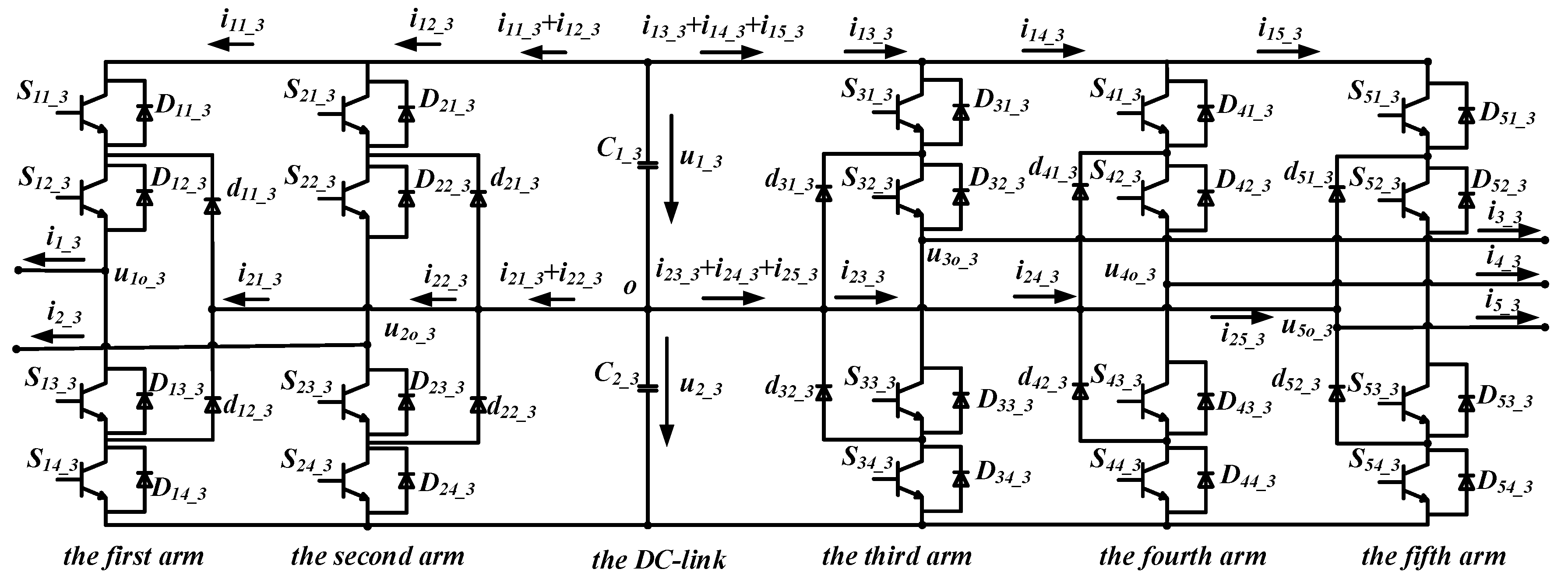
3. Model of AC-DC-AC Converter

There are $n-1$ capacitances in the DC-link of n-level AC-DC-AC converter, the model of the DC-link is built based on state space description as follows:

$$\left\{\begin{array}{c}\frac{d{u}_{1\_n}}{dt}=\frac{-{\displaystyle \sum _{x=1}^{m_n}}{i}_{1x\_n}}{C_{1\_n}}\hfill \\ \frac{d{u}_{2\_n}}{dt}=\frac{-{\displaystyle \sum _{x=1}^{m_n}}{i}_{2x\_n}}{C_{2\_n}}\hfill \\ \dots \hfill \\ \frac{d{u}_{(n-1)\_n}}{dt}=\frac{-{\displaystyle \sum _{x=1}^{m_n}}{i}_{(n-1)x\_n}}{C_{(n-1)\_n}}\hfill \end{array}\right.$$

(5)

where $C_{1\_n}$, $C_{2\_n}$...$C_{(n-1)\_n}$ are the capacitances in the DC-link from top to bottom.

The AC-DC-AC converter consists of the rectifier, inverter and the DC-link. The rectifier and inverter have $m_n$ arms in total. Combining the single arm model and the DC-link model, the model of the converter is built, which can simulate the system characters when open-circuit faults occurr in any power devices on any arms in the converter. For using real-time simulation, the model of n-level converter should be solved first [28]. Euler’s method is chosen as the numerical solver in this paper. The model of n-level converter is solved by Euler’s method, which is shown in Equation (6). $\tau$ is the size of time step for real-time simulation. Then, the timing of the model should be analyzed by static timing analysis [29]. After the timing constraints are satisfied, the model can run without a conflict of timing. It can be used to acquire the open-circuit faults data and features of n-level converter expediently.

$$\left\{\begin{array}{c}{u}_{1o\_n}\left(k+1\right)={\displaystyle \sum _{k=1}^{n-1}}{f}_k(c_{1\_n},q_{11\_n}\dots q_{1\left(2n-4\right)\_n},s_{11\_n}\dots s_{1\left(2n-2\right)\_n})u_{k\_n}\left(k+1\right)\hfill \\ u_{2o\_n}\left(k+1\right)={\displaystyle \sum _{k=1}^{n-1}}{f}_k(c_{2\_n},q_{21\_n}\dots q_{2\left(2n-4\right)\_n},s_{21\_n}\dots s_{2\left(2n-2\right)\_n})u_{k\_n}\left(k+1\right)\hfill \\ \dots \hfill \\ u_{\left(n-1\right)o\_n}\left(k+1\right)={\displaystyle \sum _{k=1}^{n-1}}{f}_k(c_{m_n\_n},q_{m_{n}1}\dots q_{m_n\left(2n-4\right)\_n},s_{m_{n}1}\dots s_{m_n\left(2n-2\right)\_n})u_{k\_n}\left(k+1\right)\hfill \\ {u^{\prime }}_{1\_n}\left(t_k\right)=\frac{-{\displaystyle \sum _{x=1}^{m_n}}{g}_1(c_{x\_n},q_{x1\_n}\dots q_{x\left(2n-4\right)\_n},s_{x1\_n}\dots s_{x\left(2n-2\right)\_n})i_{x\_n}\left(t_k\right)}{C_{1\_n}}\hfill \\ u_{1\_n}\left(k+1\right)=u_{1\_n}\left(k\right)+\tau ·{u^{\prime }}_{1\_n}\left(t_k\right)\hfill \\ {u^{\prime }}_{2\_n}\left(t_k\right)=\frac{-{\displaystyle \sum _{x=1}^{m_n}}{g}_2(c_{x\_n},q_{x1\_n}\dots q_{x\left(2n-4\right)\_n},s_{x1\_n}\dots s_{x\left(2n-2\right)\_n})i_{x\_n}\left(t_k\right)}{C_{2\_n}}\hfill \\ u_{2\_n}\left(k+1\right)=u_{2\_n}\left(k\right)+\tau ·{u^{\prime }}_{2\_n}\left(t_k\right)\hfill \\ \dots \hfill \\ {u^{\prime }}_{\left(n-1\right)\_n}\left(t_k\right)=\frac{-{\displaystyle \sum _{x=1}^{m_n}}{g}_{n-1}(c_{x\_n},q_{x1\_n}\dots q_{x\left(2n-4\right)\_n},s_{x1\_n}\dots s_{x\left(2n-2\right)\_n})i_{x\_n}\left(t_k\right)}{C_{\left(n-1\right)\_n}}\hfill \\ u_{\left(n-1\right)\_n}\left(k+1\right)=u_{\left(n-1\right)\_n}\left(k\right)+\tau ·{u^{\prime }}_{\left(n-1\right)\_n}\left(t_k\right)\hfill \end{array}\right.$$

(6)

4. Simulation and Experimental Results

The three-level converter applied in CRH2 high-speed train is chosen to verify the effectiveness and accuracy of the proposed modeling method. The topology of the converter is shown in Figure 7.

The converter model is established and solved by Euler’s method, which is shown in Equation (8).

$$\left\{\begin{array}{c}{u}_{1o\_3}(k+1)=(c_{\overline{1}\_3}{s}_{1\overline{3}\_3}+c_{1\_3}{s}_{11\_3}{s}_{12\_3}+c_{\overline{1}\_3}{q}_{1\overline{2}\_3}{s}_{12\_3}{s}_{13\_3})u_{1\_3}(k+1)\hfill \\ -(c_{1\_3}{s}_{1\overline{2}\_3}+c_{\overline{1}\_3}{s}_{13\_3}{s}_{14\_3}+c_{1\_3}{q}_{1\overline{1}\_3}{s}_{12\_3}{s}_{13\_3})u_{2\_3}(k+1)\hfill \\ u_{2o\_3}(k+1)=(c_{\overline{2}\_3}{s}_{2\overline{3}\_3}+c_{2\_3}{s}_{21\_3}{s}_{22\_3}+c_{\overline{2}\_3}{q}_{2\overline{2}\_3}{s}_{22\_3}{s}_{23\_3})u_{2\_3}(k+1)\hfill \\ -(c_{2\_3}{s}_{2\overline{2}\_3}+c_{\overline{2}\_3}{s}_{23\_3}{s}_{24\_3}+c_{2\_3}{q}_{2\overline{1}\_3}{s}_{22\_3}{s}_{23\_3})u_{2\_3}(k+1)\hfill \\ \dots \hfill \\ u_{5o\_3}(k+1)=(c_{\overline{5}\_3}{s}_{5\overline{3}\_3}+c_{5\_3}{s}_{51\_3}{s}_{52\_3}+c_{\overline{5}\_3}{q}_{5\overline{2}\_3}{s}_{52\_3}{s}_{53\_3})u_{1\_3}(k+1)\hfill \\ -(c_{5\_3}{s}_{5\overline{2}\_3}+c_{\overline{5}\_3}{s}_{53\_3}{s}_{54\_3}+c_{5\_3}{q}_{5\overline{1}\_3}{s}_{52\_3}{s}_{53\_3})u_{2\_3}(k+1)\hfill \\ u_{1\_3}^{\prime }=\frac{-{\displaystyle \sum _{x=1}^5}(c_{\overline{x}\_3}{s}_{x\overline{3}\_3}+c_{x\_3}{s}_{x1\_3}{s}_{x2\_3}+c_{\overline{x}\_3}{q}_{x\overline{2}\_3}{s}_{x2\_3}{s}_{x3\_3})i_{x\_3}\left(t_k\right)}{C_{1\_3}}\hfill \\ u_{1\_3}(k+1)=u_{1\_3}\left(k\right)+\tau ·u_{1\_3}^{\prime }\left(t_k\right)\hfill \\ u_{2\_3}^{\prime }=\frac{-{\displaystyle \sum _{x=1}^5}(c_{x\_3}{q}_{x1\_3}{s}_{x\overline{1}\_3}{s}_{x2\_3}+c_{\overline{x}\_3}{q}_{x2\_3}{s}_{x3\_3}{s}_{x\overline{4}\_3})i_{x\_3}\left(t_k\right)}{C_{2\_3}}\hfill \\ u_{2\_3}(k+1)=u_{2\_3}\left(k\right)+\tau ·u_{2\_3}^{\prime }\left(t_k\right)\hfill \end{array}\right.$$

(7)

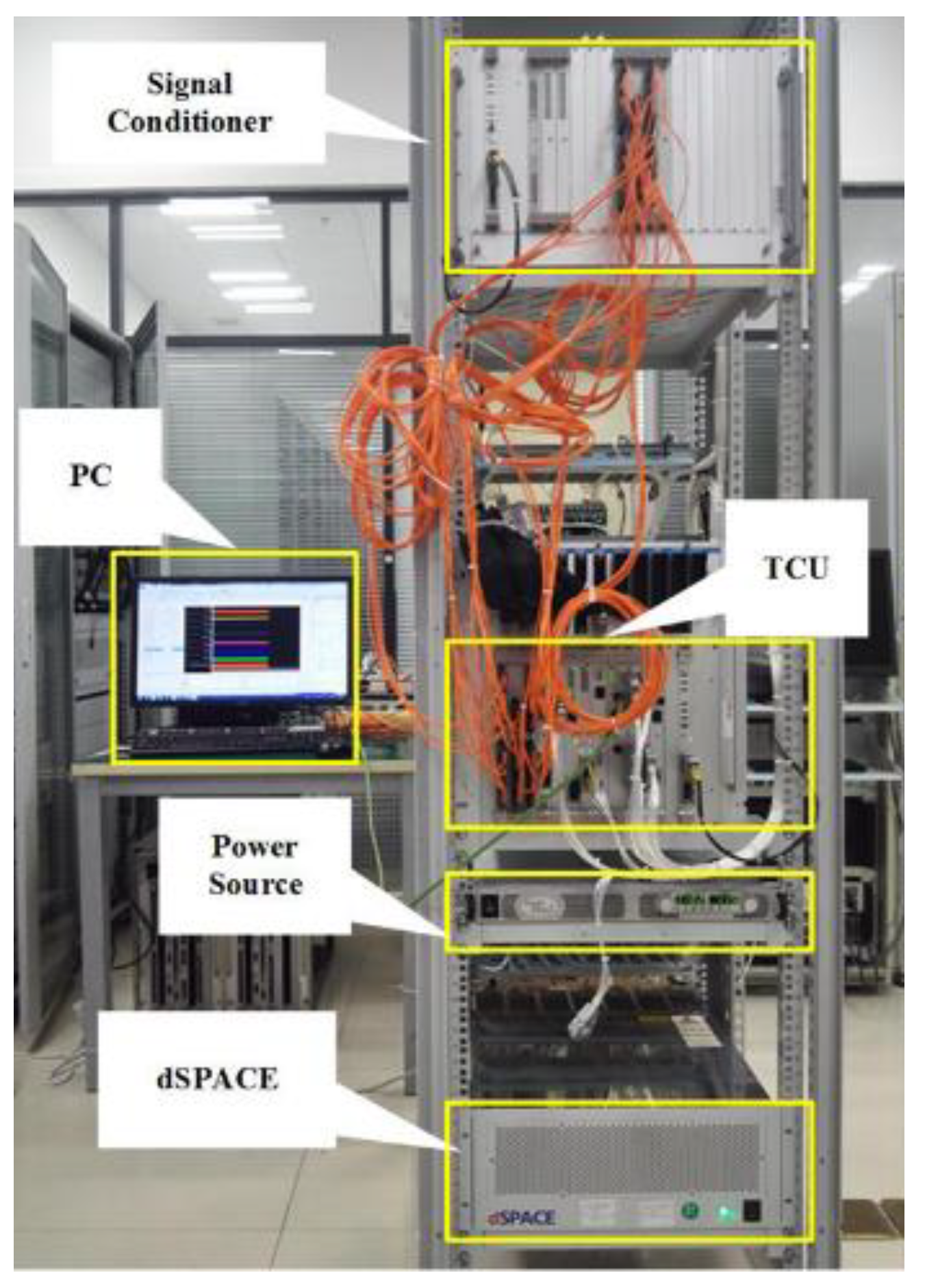
Two testing platforms of a three-level converter are constructed. One is the off-line simulation platform built by commercial encapsulated modules, the time step is 10 us. All parts of the platform are realized in personal computer (PC) and the calculation speed is slow. The software package of this platform is developed [21,30]. 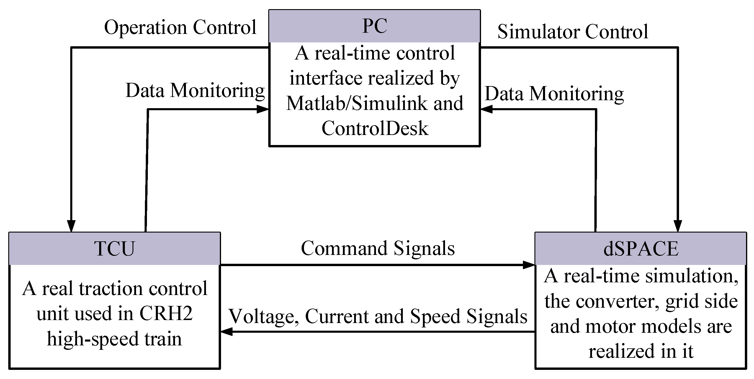The other is the HIL-based experimental platform established in a Chinese high-speed train manufacturer’s laboratory, which is shown in Figure 8. A grid side supply to the converter and a traction motor are applied as the load. The experimental platform comprises a real traction control unit (TCU) used in CRH2 high-speed trains, and a computer as a real-time control interface. The hardware circuit, including the model of three-level converter, the grid side model, the traction motor model and the sensors are realized in dSPACE, which is a real-time simulator controlled by the ControlDesk. The open-circuit faults are introduced by changing the command signals of power devices to zero. The TCU gets the current, voltage and speed signals from the dSPACE and sends the command signals to the dSPACE after the A/D conversion and calculations. Combining the Matlab/Simulink and ControlDesk, the real-time control is realized, the time step of the whole system monitoring is 40 us. The models operating in the dSPACE at a time step of 10 ns. The relationship between different parts of the experimental platform is shown in Figure 9. A comparison between off-line simulation platform and experimental platform is shown in

Table 3. Comparison between off-line simulation platform and experimental platform.

Comparison Item	HIL-Based Experimental Platform	Off-Line Simulation Platform
TCU	real TCU	realized in PC
Converter, grid side and motor	mathematical models realized in dSPACE	commercial encapsulated modules realized in PC
Sensor network	realized in dSPACE	realized in PC
Calculation mode	parallel mode	serial mode
Time step	10 ns	10 us
Timeliness	fast	slow
Real-time	yes	no

. The parameters of the grid side and converter are given in

Table 4. Parameters of converter.

Parameter	Symbol	Value
RMS grid voltage	$u_N$	1500 V
Traction winding leakage inductor	$L_N$	2 mH
Traction winding leakage resistor	$R_N$	0.2 Ω
DC-link voltage	$u_1$, $u_2$	1300 V
DC-link capacitor	$C_1$, $C_2$	16 mF

, and the parameters of the traction motor are given in

Table 5. Parameters of traction motor.

Parameter	Symbol	Value
Stator resistance	$R_s$	0.15 Ω
Stator leakage inductance	$L_{ls}$	1.42 mH
Rotor resistance	$R_r$	0.16 Ω
Rotor leakage inductance	$L_{lr}$	0.6 mH
Mutual inductance	$L_m$	25.4 mF
Rated voltage	$U_{rate}$	2000 V
Rated frequency	$f_{rate}$	140 Hz
Rated speed	$n_{rate}$	4140 r/min
Rated output power	$P_{rate}$	300 kW
Rated slip frequency	$s_{rate}$	1.4%
Number of the pole pairs	$n_P$	2

.

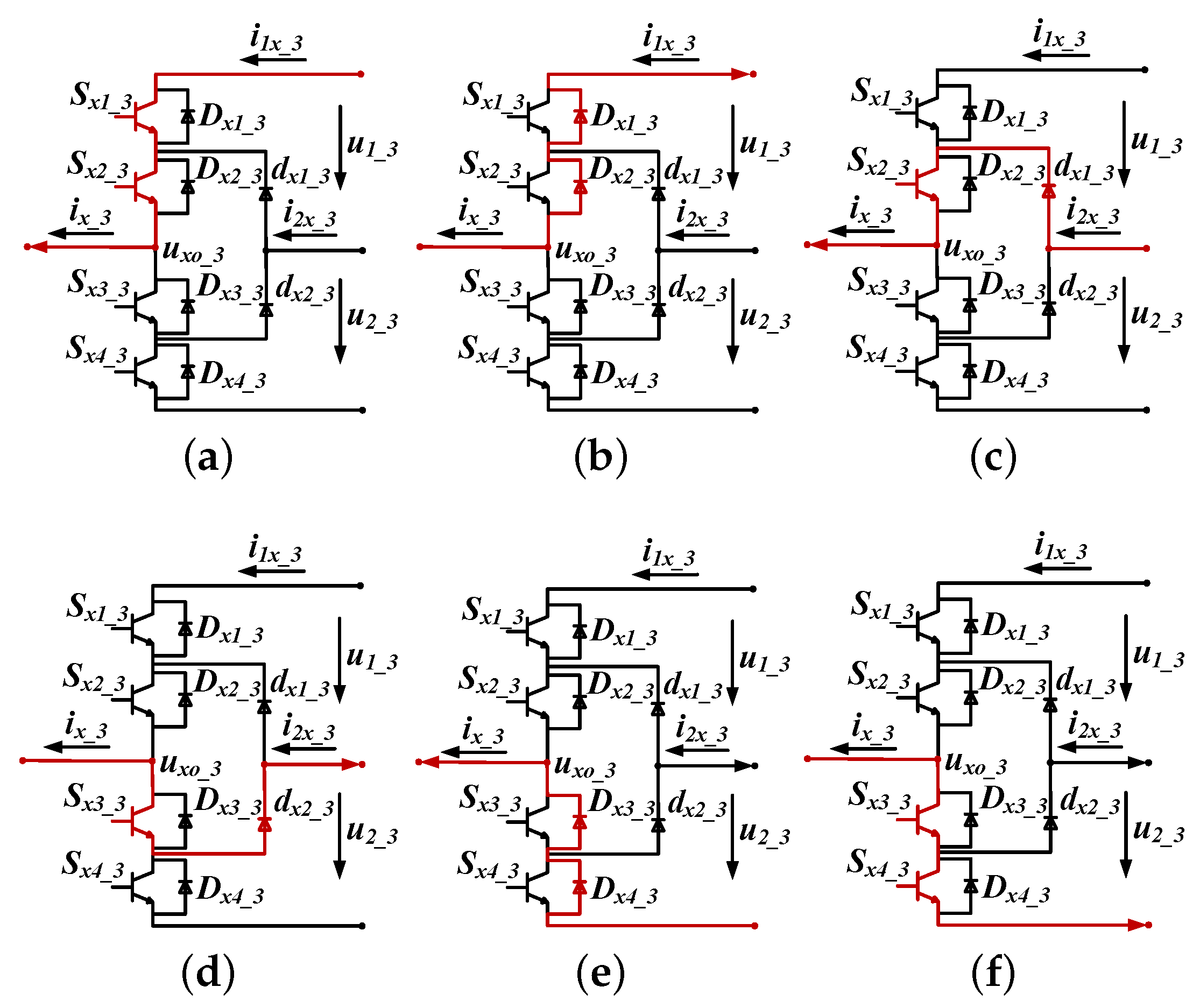
4.1. Open-Circuit Faults in Rectifier

The first arm and second arm are in the rectifier. Because of structural symmetry, the phenomena of open-circuit faults happening in the second arm are similar to open-circuit faults occurring in the first arm. For the rectifier, take the first arm as an example, the results of open-circuit faults are given in Figure 10. The results are consistent with theoretical analysis. When open-circuit faults occur in $S_{11\_3}$, the current paths are changed while $i_{1\_3}$ is positive, so $i_{1\_3}$ is influenced in positive phase. The peak value of positive phase decreases, but the fault has little effect on $i_{1\_3}$ in negative phase, which is shown in Figure 10a. When open-circuit faults happen in $S_{12\_3}$, the current paths are changed seriously while $i_{1\_3}$ is positive, so the positive phase of $i_{1\_3}$ is almost cut off. If $i_{1\_3}$ is negative, the current paths do not include $S_{12\_3}$, but in order to stable the power of the three-level converter, the peak value of the negative phase increases, as shown in Figure 10b. When open-circuit faults occur in $d_{11\_3}$, the influence on $i_{1\_3}$ is similar to $S_{12\_3}$, as shown in Figure 10e. The analysis of open-circuit faults occurring in $S_{13\_3}$, $S_{14\_3}$, and $d_{12\_3}$ is similar to open-circuit faults happening in $S_{12\_3}$, $S_{11\_3}$, and $d_{11\_3}$, respectively. The results are shown in Figure 10c,d,f.

4.2. Open-Circuit Faults in Inverter

The third arm, fourth arm and the fifth arm are in the inverter and have the same structure. The system characteristics of open-circuit faults happening in the fourth arm and the fifth arm are similar to open-circuit faults occurring in the third arm. For the inverter, the third arm is chosen as a representative, the results of open-circuit faults in $S_{31\_3}$, $S_{32\_3}$, $S_{33\_3}$, $S_{34\_3}$, $d_{31\_3}$, and $d_{32\_3}$ are given in Figure 11. The influences of open-circuit faults happening in the third arm are similar to the first arm, but there are three main differences. First, when open-circuit faults occur in $S_{31\_3}$ or $S_{34\_3}$, the effect in positive or negative phase are more serious. Second, the inverter is a three-phase supply, when open-circuit faults occur in $S_{32\_3}$ or $S_{33\_3}$, although the positive or negative phase is almost cut off, two other phase supplies can provide enough power, the park value of negative or positive phase does not increase obviously. Third, when open-circuit faults occur in $d_{31\_3}$, and $d_{32\_3}$, the influences are similar to $S_{31\_3}$ and $S_{34\_3}$, respectively.

The simulation results are obtained by the off-line simulation platform, which is built by commercial encapsulated modules and cannot be used for real-time simulation. The experiment results are acquired by the experimental platform established in a Chinese high-speed train manufacturer’s laboratory, which includes the physical TCU and a real-time simulator. The proposed model is realized in the real-time simulator. The relative error is defined as follows:

$$\delta =\left|\frac{\mathrm{experiment}\mathrm{result}-\mathrm{simulation}\mathrm{result}}{\mathrm{simulation}\mathrm{result}}\right|\times 100\%$$

(8)

When an open-circuit fault occurs, the most obvious change is peak to peak values of the phase current. The δ of peak to peak values in normal condition are shown in

Table 6. Relative error of phase current in normal condition.

Variables	$\mathit{\delta }$
$i_{1\_3}$	2.1%
$i_{2\_3}$	2.1%
$i_{3\_3}$	1.0%
$i_{4\_3}$	1.0%
$i_{5\_3}$	1.3%

. The δ of peak to peak values in $i_{1\_3}$ after open-circuit faults occur in first arm and the δ of peak to peak values in $i_{3\_3}$ after open-circuit faults occur in third arm are shown in

Table 7. Relative error of phase current with open-circuit fault.

Variables	Fault Location	$\mathit{\delta }$
$i_{1\_3}$	$S_{11\_3}$	3.1%
	$S_{12\_3}$	4.3%
	$S_{13\_3}$	4.5%
	$S_{14\_3}$	3.3%
	$d_{11\_3}$	4.3%
	$d_{12\_3}$	4.6%
$i_{3\_3}$	$S_{31\_3}$	2.3%
	$S_{32\_3}$	4.2%
	$S_{33\_3}$	4.3%
	$S_{34\_3}$	2.6%
	$d_{31\_3}$	2.5%
	$d_{32\_3}$	2.8%

. The δ are less than 5% in all conditions, which validates effectiveness and accuracy of the modeling method proposed in this paper.

4.3. Comparison with Existing Models

The comparison between the proposed converter model and existing converter models is summarized in

Table 8. Comparison between proposed model and existing models.

Converter Model	Mathematical Model	Open-Circuit Fault Location	Real-Time Simulation	Portability	Uniformity
Circuit model [21]	no	power devices	no	yes	yes
Switching function-based model [14,15,16,17]	yes	no	yes	no	no
Controlled source-based model [18,19,20]	yes	no	yes	no	no
uniform model [24]	yes	power devices	yes	no	yes
Proposed model	yes	power devices and clamping diodes	yes	yes	yes

. There are five indexes: Mathematical model (is it a mathematical model?); open-circuit faults location (which locations of open-circuit faults can be simulated?); real-time simulation (can it be used for real-time simulation?); portability and uniformity. As we can see in the table, the proposed model has good performance in the indexes mentioned above and the existing models have some shortcomings.

5. Conclusions

A modeling method for a power converter, which can express the converter in abnormal conditions in which an open-circuit fault occurs in power devices and clamping diodes, is presented in this paper. The key of the method is the single arm model, which has good portability. In the modeling process, only a single arm needs to be analyzed instead of the whole power converter. The inputs and outputs are redefined making the single arm model easy to be built. Once the single arm model is established, it can be used to build all the power converters which have arms with the same structure. An AC-DC-AC converter is chosen as an example to explain the modeling method and a general model of AC-DC-AC converter is built. The simulation and experiment results confirm the effectiveness and accuracy of the proposed model. Compared with the switching function-based model and controlled source-based model, the proposed model can simulate the converter with open-circuit faults. Unlike the circuit model, the proposed one is a mathematical model and can be applied to the hardware-in-the-loop simulation. A real-time fault injection platform of converter used in the traction control system has been built in a Chinese high-speed train manufacturer’s laboratory, which is a more reliable environment and offers more authentic data for open-circuit fault detection, diagnosis and tolerant control.

References

1. Wang, H.; Liserre, M.; Blaabjerg, F.; Rimmen, P.P.; Jacobsen, J.B. Transitioning to Physics-of-Failure as a Reliability Driver in Power Electronics. IEEE J. Emerg. Sel. Top. Power Electron. 2014, 2, 97–114. [Google Scholar] [CrossRef]
2. Albatran, S.; Smadi, I.A.; Ahmad, H.J.; Koran, A. Online Optimal Switching Frequency Selection for Grid-Connected Voltage Source Inverters. Electronics 2017, 6, 110. [Google Scholar] [CrossRef]
3. Yamamoto, E.; Hara, H.; Uchino, T.; Kawaji, M.; Kume, T.J.; Kang, J.K.; Krug, H. Development of MCs and its Applications in Industry [Industry Forum]. IEEE Ind. Electron. Mag. 2011, 5, 4–12. [Google Scholar] [CrossRef]
4. Bagnoli, P.E.; Casarosa, C.; Ciampi, M.; Dallago, E. Thermal resistance analysis by induced transient (TRAIT) method for power electronic devices thermal characterization. I. Fundamentals and theory. IEEE Trans. Power Electron. 1998, 13, 1208–1219. [Google Scholar] [CrossRef]
5. Yang, S.; Xiang, D.; Bryant, A.; Mawby, P.; Ran, L.; Tavner, P. Condition Monitoring for Device Reliability in Power Electronic Converters: A Review. IEEE Trans. Power Electron. 2010, 25, 2734–2752. [Google Scholar] [CrossRef]
6. Ribeiro, E.; Cardoso, A.M.; Boccaletti, C. Open-Circuit Fault Diagnosis in Interleaved DC-DC Converters. IEEE Trans. Power Electron. 2014, 29, 3091–3102. [Google Scholar] [CrossRef]
7. Nuutinen, P.; Peltoniemi, P.; Silventoinen, P. Short-Circuit Protection in a Converter-Fed Low-Voltage Distribution Network. IEEE Trans. Power Electron. 2013, 28, 1587–1597. [Google Scholar] [CrossRef]
8. Choi, U.; Jeong, H.; Lee, K.; Blaabjerg, F. Method for Detecting an Open-Switch Fault in a Grid-Connected NPC Inverter System. IEEE Trans. Power Electron. 2012, 27, 2726–2739. [Google Scholar] [CrossRef]
9. Lu, B.; Sharma, S.K. A Literature Review of IGBT Fault Diagnostic and Protection Methods for Power Inverters. IEEE Trans. Ind. Appl. 2009, 45, 1770–1777. [Google Scholar]
10. Abari, I.; Lahouar, A.; Hamouda, M.; Ben Hadj Slama, J.; Al-Haddad, K. Fault Detection Methods for Three-Level NPC Inverter based on DC Bus Electromagnetic Signatures. IEEE Trans. Ind. Electron. 2018, 65, 5224–5236. [Google Scholar] [CrossRef]
11. Rosa, A.R.; Silva, M.E.; Campos, F.C.; Santana, R.S.; Rodrigues, W.A.; Morais, L.F.; Seleme, S.I., Jr. SHIL and DHIL Simulations of Nonlinear Control Methods Applied for Power Converters Using Embedded Systems. Electronics 2018, 7, 241. [Google Scholar] [CrossRef]
12. Guo, X.; Yuan, J.; Tang, Y.; You, X. Hardware in the Loop Real-time Simulation for the Associated Discrete Circuit Modeling Optimization Method of Power Converters. Energies 2018, 11, 3237. [Google Scholar] [CrossRef]
13. Zhang, H.; Zhang, Y.; Yin, C. Hardware-in-the-Loop Simulation of Robust Mode Transition Control for a Series-Parallel Hybrid Electric Vehicle. IEEE Trans. Veh. Technol. 2016, 65, 1059–1069. [Google Scholar] [CrossRef]
14. Ngo, V.; Nguyen, M.; Tran, T.; Choi, J.; Lim, Y. A Modified Model Predictive Power Control for Grid-Connected T-Type Inverter with Reduced Computational Complexity. Electronics 2019, 8, 217. [Google Scholar] [CrossRef]
15. Ye, Z.; Xu, Y.; Wu, X.; Tan, G.; Deng, X.; Wang, Z. A Simplified PWM Strategy for a Neutral-Point-Clamped (NPC) Three-Level Converter With Unbalanced DC Links. IEEE Trans. Power Electron. 2016, 31, 3227–3238. [Google Scholar] [CrossRef]
16. Aciego, J.J.; Gonzalez-Prieto, I.; Duran, M.J. Model Predictive Control of Six-phase Induction Motor Drives Using Two Virtual Voltage Vectors. IEEE J. Emerg. Sel. Top. Power Electron. 2019, 7, 321–330. [Google Scholar] [CrossRef]
17. Liu, X.; Cramer, A.M.; Pan, F. Generalized Average Method for Time-Invariant Modeling of Inverters. IEEE Trans. Circuits Syst. I-Regul. Pap. 2017, 64, 740–751. [Google Scholar] [CrossRef]
18. Wang, X.; Blaabjerg, F.; Liserre, M.; Chen, Z.; He, J.; Li, Y. An Active Damper for Stabilizing Power-Electronics-Based AC Systems. IEEE Trans. Power Electron. 2014, 29, 3318–3329. [Google Scholar] [CrossRef]
19. Wang, X.; Blaabjerg, F.; Wu, W. Modeling and Analysis of Harmonic Stability in an AC Power-Electronics-Based Power System. IEEE Trans. Power Electron. 2014, 29, 6421–6434. [Google Scholar] [CrossRef]
20. Wang, R.; Wu, Y.; He, G.; Lv, Y.; Du, J.; Li, Y. Impedance Modeling and Stability Analysis for Cascade System of Three-Phase PWM Rectifier and LLC Resonant Converter. Energies 2018, 11, 3050. [Google Scholar] [CrossRef]
21. Yang, C.; Yang, C.; Peng, T.; Yang, X.; Gui, W. A Fault-Injection Strategy for Traction Drive Control System. IEEE Trans. Ind. Electron. 2017, 64, 5719–5727. [Google Scholar] [CrossRef]
22. Chen, Z.; Ding, S.X.; Peng, T.; Yang, C.; Gui, W. Fault Detection for Non-Gaussian Processes Using Generalized Canonical Correlation Analysis and Randomized Algorithms. IEEE Trans. Ind. Electron. 2018, 65, 1559–1567. [Google Scholar] [CrossRef]
23. Chen, Z.; Yang, C.; Peng, T.; Dan, H.; Li, C.; Gui, W. A cumulative canonical correlation analysis-based sensor precision degradation detection method. IEEE Trans. Ind. Electron. 2019, 66, 6321–6330. [Google Scholar] [CrossRef]
24. Peng, T.; Tao, H.; Yang, C.; Chen, Z.; Yang, C.; Gui, W.; Karimi, H.R. A Uniform Modeling Method Based on Open-Circuit Faults Analysis for NPC-Three-Level Converter. IEEE Trans. Circuits Syst. II-Express Briefs 2019, 66, 457–461. [Google Scholar] [CrossRef]
25. Rocha, N.; da Costa, A.E.L.; Jacobina, C.B. Parallel of Two Unidirectional AC-DC-AC Three-Leg Converters to Improve Power Quality. IEEE Trans. Power Electron. 2018, 33, 7782–7794. [Google Scholar] [CrossRef]
26. Maia, A.C.N.; Jacobina, C.B. Single-phase ac-dc-ac topology for grid overvoltage and voltage harmonic mitigation. IET Power Electron. 2017, 10, 1626–1637. [Google Scholar] [CrossRef]
27. Song, W.; Ma, J.; Zhou, L.; Feng, X. Deadbeat Predictive Power Control of Single-Phase Three-Level Neutral-Point-Clamped Converters Using Space-Vector Modulation for Electric Railway Traction. IEEE Trans. Power Electron. 2016, 31, 721–732. [Google Scholar] [CrossRef]
28. Yang, X.; Yang, C.; Peng, T.; Chen, Z.; Liu, B.; Gui, W. Hardware-in-the-Loop Fault Injection for Traction Control System. IEEE J. Emerg. Sel. Top. Power Electron. 2018, 6, 696–706. [Google Scholar] [CrossRef]
29. Huang, T.; Wong, M.D.F. UI-Timer 1.0: An Ultrafast Path-Based Timing Analysis Algorithm for CPPR. IEEE Trans. Comput-Aided Des. Integr. Circuits Syst. 2016, 35, 1862–1875. [Google Scholar] [CrossRef]
30. Yang, C. Fault-Injection Benchmark Platform for Traction Drive Control System (TDCS_FIB). Available online: http://gfist.csu.edu.cn/downloadE.html (accessed on 26 April 2016).
Figure 1. The topology of a single two-level arm.
Electronics 08 00633 g001
Figure 2. Inputs and outputs of a single two-level arm.
Electronics 08 00633 g002
Figure 3. Current paths in a single two-level arm.
Electronics 08 00633 g003
Figure 4. The topology of a single three-level arm.
Electronics 08 00633 g004
Figure 5. Current paths in a single three-level arm.
Electronics 08 00633 g005
Figure 6. Topology of a single five-level arm.
Electronics 08 00633 g006
Figure 7. The topology of three-level converter.
Electronics 08 00633 g007
Figure 8. The HIL-based experimental platform.
Electronics 08 00633 g008
Figure 9. The relationship between different parts of the HIL-based experimental platform.
Electronics 08 00633 g009
Figure 10. Results of open-circuit faults happening in the first arm.
Electronics 08 00633 g010
Figure 11. Results of open-circuit faults happening in the third arm.
Electronics 08 00633 g011