Article

Sub-Aperture Partitioning Method for Three-Dimensional Wide-Angle Synthetic Aperture Radar Imaging with Non-Uniform Sampling

1
State Key Laboratory of Complex Electromagnetic Environment Effects on Electronics and Information System, National University of Defense Technology, Changsha 410073, China
2
College of Electronic Science, National University of Defense Technology, Changsha 410073, China
*
Author to whom correspondence should be addressed.
Electronics 2019, 8(6), 629; https://doi.org/10.3390/electronics8060629
Submission received: 28 April 2019 / Revised: 2 June 2019 / Accepted: 2 June 2019 / Published: 3 June 2019
(This article belongs to the Section Microwave and Wireless Communications)

Abstract

:
For a three-dimensional wide-angle synthetic aperture radar (SAR) with non-uniform sampling, it is necessary to divide its large aperture into several small sub-apertures before imaging due to the anisotropic characteristics of the target. The existing sub-aperture partitioning methods divide the aperture with equal intervals. However, for the non-uniformly sampled SAR, those equal-interval partitioning methods may have a bad effect on the resolution of the SAR imaging result. In view of this, a sub-aperture partitioning method for three-dimensional wide-angle SAR imaging with non-uniform sampling was proposed in this paper. First, we analyzed the relationship between the three-dimensional resolution and the sampling distribution in K-space based on the Cramer–Rao lower bound. Subsequently, according to the distribution of K-space sampling, the optimum size of each sub-aperture was found and the aperture was divided non-uniformly. Furthermore, the proposed method was validated by electromagnetic simulation data. The proposed sub-aperture partitioning method ensured that the resolution of each sub-aperture was high and consistent. By comparing with the equal-interval partitioning method, the experimental results showed that our proposed method had a higher resolution imaging result.

1. Introduction

Synthetic aperture radar (SAR) is an active microwave imaging sensor, which has the advantage of all-day and all-weather observation. In recent years, acquiring more comprehensive information from the target has become the development trend of SAR [1,2,3]. Compared with the conventional SAR, three-dimensional (3-D) SAR such as tomographic SAR (Tomo-SAR) and interferometric SAR can acquire 3-D scattering information of the target and overcome the distortion such as layover and shadow [4,5]. Wide-angle SAR such as circular SAR can acquire more azimuth information of the target and get anisotropic characteristics of the target [6,7,8]. Combining 3-D SAR with wide-angle SAR is bound to obtain more comprehensive information of the target, thus conducive to improving the accuracy of target recognition and terrain classification.
3-D wide-angle SAR data can be acquired by Tomo-SAR, whose flight trajectories are delineated in Figure 1 by cyan dotted lines. Uniform and dense sampling of Tomo-SAR makes data collection time-consuming and high-cost [9,10]. However, 3-D wide-angle SAR data can be obtained through the non-linear flight of SAR, which reduces the cost of data acquisition greatly [11,12,13]. On this basis, an effective way to collect data is based on the non-linear flight paths, which is generated by the cooperative flight of multiple small unmanned aerial vehicles (UAVs) with SAR system installed [14,15,16]. The curve trajectory in Reference [9] is used as the trajectories for UAVs. As shown in Figure 1, the green, red, blue, yellow and black curves represent the flight trajectories of five UAVs, respectively. Also, the data sampling is not uniformly distributed on these five flight trajectories.
It is known that a large azimuth accumulation angle is a remarkable feature of 3-D wide-angle SAR with non-uniform sampling. Generally, the scatterer is assumed to be isotropic when imaging for SAR with a small azimuth accumulation angle. However, the isotropic scattering assumption is invalid for most scattering centers in the scene for wide-angle SAR [7,17]. Therefore, the anisotropic characteristics of the target needs to be considered in a 3-D wide-angle SAR imaging method. In order to solve the problem, there are two processing methods commonly used in 3-D wide-angle SAR imaging.
One is the full-aperture processing method. It models the target scattering as a function of space and viewing angle, also, full-aperture data are employed for imaging directly [18,19]. However, the computational complexity of this method is large [17]. The other is the sub-aperture processing method. It divides the large aperture into smaller sub-apertures whose scatterers are almost isotropic. After imaging on each sub-aperture, the sub-images are appropriately combined together to reconstruct the full-aperture imaging results [7,8,17]. In summary, by comparing with the full-aperture processing method, the sub-aperture processing method has less computation and better adaptability and wider applications [17].
In the existing sub-aperture processing methods [17,20,21], the aperture was divided with equal intervals (constant sub-aperture size and overlapping size) to ensure that the information on each line of sight was included and the resolution of each sub-aperture was the same. Although this equal-interval partitioning method is suitable for uniformly sampled SAR. However, the sub-aperture partitioning problem under non-uniform sampling has not been well solved. In fact, for non-uniformly sampled SAR, the existing sub-aperture processing approaches are not appropriate since the same resolution of each sub-aperture cannot be guaranteed when dividing the aperture with equal intervals.
The sampling distribution in K-space (spatial frequency domain) affects the resolution of the imaging result. Specifically, Moore et al. demonstrated that a greater diversity of K-space samples produced a higher 3-D resolution [22]. Figure 2 shows the K-space sampling of Tomo-SAR and five cooperative UAVs with the associated SAR system referred to in Figure 1. It can be seen that the K-space sampling of Tomo-SAR was uniform while that of UAVs with the SAR system was non-uniform. For uniform K-space sampling, when dividing the aperture with equal intervals, the resolution of each sub-aperture is the same due to the same distribution in different sub-apertures. However, for non-uniformly sampled data as described above, the equal-interval partitioning will lead to a different resolution for each sub-aperture due to the different distributions of K-space sampling in different sub-apertures, and also make the resolution of the SAR imaging result even worse. Therefore, with the aim of obtaining higher resolution imaging results for 3-D wide-angle SAR with non-uniform sampling, a non-uniform sub-aperture partitioning method is urgently needed to ensure the consistency of the resolution for each sub-aperture.
In this paper, we divided the aperture appropriately to get a higher resolution imaging result for 3-D wide-angle SAR with non-uniform sampling. First, we analyzed the relationship between the 3-D resolution and the sampling distribution in K-space based on the Cramer–Rao lower bound (CRLB) of 3-D position estimation error. Then, the distribution of k-space sampling was taken into account when dividing the aperture and a non-uniform sub-aperture partitioning method was proposed, which yielded high and consistent resolution for each sub-aperture. The resolution of the SAR imaging result obtained by the proposed method was much better than that of the equal-interval partitioning method.
The outline of the paper is illustrated as follows: Section 1 introduces the background of sub-aperture partitioning and the structure of this paper; Section 2 and Section 3 present the signal model and the 3-D resolution estimation based on CRLB; Section 4 introduces the 3-D wide-angle SAR imaging with non-uniform sampling; Section 5 provides the procedure of the proposed non-uniform sub-aperture partitioning method, which was designed based on contents from Section 2, Section 3 and Section 4; Experimental results and conclusions are shown in Section 6 and Section 7, respectively.

2. Signal Model

It is known that the assumption of isotropic scattering is invalid for the 3-D wide-angle SAR with non-uniform sampling. On this basis, the 3-D scattering model [22] of the point target at the location ( x , y , z ) should be expressed as:
Y = S + n = A e j φ e j ( k x x + k y y + k z z ) p α ( θ ) + n .
where, S represents the scattering model without noise, A e j φ is the complex amplitude of the target, α is the scattering persistence of the target, and p α ( θ ) is a window function. When azimuth | θ | α / 2 , p α ( θ ) = 1 , otherwise p α ( θ ) = 0 . n is Gauss white noise with variance σ 2 , and the sampling position in K-space is given by [9]:
k x = 4 π f c cos θ cos ϕ k y = 4 π f c cos θ sin ϕ k z = 4 π f c sin θ
where c is the speed of light, the frequency, azimuth and elevation of the radar are respectively represented by f , θ , ϕ .
The essence of imaging is to estimate parameter Θ = [ A , α , φ , x , y , z ] T from Y . As a consequence, the 3-D resolution of the imaging results can be reflected by the CRLB for parameter Θ estimation.

3. 3-D Resolution Estimation Based on Cramer–Rao Lower Bound (CRLB)

The K-space sampling is non-uniform and has a wide range for the 3-D wide-angle SAR with non-uniform sampling, as shown in Figure 2b. Therefore, the 3-D resolution of the imaging result cannot be determined by the size of the bandwidth and accumulation angle as usual. As a matter of fact, the CRLB of the position estimation error has the ability to predict the resolution with a given sensor distribution [22]. On this basis, we analyzed the relationship between the 3-D resolution and the sampling distribution in K-space based on the CRLB of the 3-D position estimation error.
The CRLB for parameter Θ estimation was defined as in [23]:
C R L B = I Θ 1
where I Θ is the Fisher information matrix. Each element of I Θ is given by [23]:
I Θ i j = E { ( ln P ( Y | Θ ) Θ i ) ( ln P ( Y | Θ ) Θ j ) T }
According to the 3-D scattering model represented in Equation (1), it is known that Y follows the distribution as P ( Y | Θ ) ~ C N ( S , σ 2 I ) , and
ln P ( Y | Θ ) = N ln ( π σ 2 ) 1 σ 2 ( Y S ) T ( Y S )
where N represents the number of sampling in K-space.
Combining Equation (1) and Equation (5) with Equation (4), the Fisher information matrix was simplified as:
I Θ = 2 N A 2 σ 2 [ A 2 0 0 0 0 0 0 0 0 0 0 0 0 0 1 μ x μ y μ z 0 0 μ x 0 0 μ y R 0 0 μ z ]
where μ x , μ y , μ z represent the centers of sampling in K-space, and R is cross-correlation matrix sampled in K-space. The expressions of μ x , μ y , μ z and R are as follows:
μ x = 1 N α n = 1 N α ( k x n p α ( θ ) ) , μ y = 1 N α n = 1 N α ( k y n p α ( θ ) ) , μ z = 1 N α n = 1 N α ( k z n p α ( θ ) )
R = 1 N α n = 1 N α [ k x n p α ( θ ) , k y n p α ( θ ) , k z n p α ( θ ) ] T [ k x n p α ( θ ) , k y n p α ( θ ) , k z n p α ( θ ) ]
where N α is the number of sampling in K-space within the extent of the window function p α ( θ ) .
Furthermore, after partitioning Fisher information matrix, the CRLB sub-matrix C R L B x y z of the target position ( x , y , z ) was obtained through matrix decomposition and matrix inversion [24]
C R L B x y z = σ 2 2 N A 2 C 1
where matrix C denotes the covariance matrix of the sampling in K-space and is expressed as:
C = R [ μ x , μ y , μ z ] T [ μ x , μ y , μ z ]
The C R L B x y z defines the uncertain range of position estimation. The square root of the determinant of C R L B x y z is proportional to the volume of the uncertain range and hence gives a measure of the resolution [22]. Therefore, the estimation of 3-D resolution was given by:
V C R L B = β det C 1
In Equation (11), the scale factor of C R L B x y z was replaced by an adjustable parameter β , which avoided the influence from the sampling number and the target scattering amplitude. Since the purpose of this paper was to propose a suitable sub-aperture partitioning method by analyzing the change of 3-D resolution in different K-spaces by Equation (11), thus the adjustable parameter β did not affect the experimental results.
Equation (11) depicts that the 3-D resolution estimation V C R L B is determined by the distribution of K-space sampling and the scattering persistence of the target. A great diversity of samples results in a higher resolution of the imaging result. In addition, when the aperture extent is larger than the scattering persistence of the target, the 3-D resolution cannot be improved with increasing aperture extent. In summary, Equation (11) can be used to predict the 3-D resolution with the given K-space sampling and target.

4. 3-D Wide-Angle SAR Imaging with Non-Uniform Sampling

The azimuth range of 3-D wide-angle SAR with non-uniform sampling is [66°, 114°], as shown in Figure 1. If full-aperture imaging is carried out directly, a better azimuth resolution is expected due to the large azimuth aperture size of 48°. However, direct full-aperture imaging leads to the weak scatterer (small scattering persistence) being covered by the strong scatterer (large scattering persistence), thus the anisotropic characteristic of the target is ignored, which will cause a mismatch between imaging result and real scene. Moreover, when the aperture extent is larger than the scattering persistence of the target, it can be deduced from Equation (11) that increasing the aperture extent does not improve the 3-D resolution anymore. Therefore, direct full-aperture imaging is sometimes unnecessary.
In order to take care of the weak scatterer, the sub-aperture processing method is used for 3-D wide-angle SAR imaging with non-uniform sampling. When using the sub-aperture processing method, the large aperture is divided into smaller sub-apertures firstly. After imaging by the 3-D non-uniform fast Fourier transform (3-D NUFFT) on each sub-aperture, the final imaging result is obtained by fusing all sub-aperture images. A feasible way for sub-aperture fusion is the generalized likelihood ratio test (GLRT) approach [9].
I ( x , y , z ) = arg max i | I ( x , y , z ; i ) |
where I ( x , y , z ; i ) represents the imaging result corresponding to the i t h sub-aperture and I ( x , y , z ) represents the final imaging result.
Remarkably, the GLRT approach requires that the resolution of each sub-aperture image is the same. If there is a sub-aperture image with poor resolution, the resolution of the final imaging result fused by the GLRT approach will also be poor. In view of this, the principle of sub-aperture partitioning is that the resolution of each sub-aperture should be consistent and the information in each line of sight should be included.
The equal-interval sub-aperture partitioning method, as the most commonly used method, divides the aperture with equal interval. In this method, the size of each sub-aperture and the overlapping between each sub-aperture were constant. However, it was not appropriate for non-uniformly sampled SAR. Since the resolution of the imaging result was influenced by the non-uniform sampling in K-space, namely, the resolution of each sub-aperture cannot be guaranteed to be the same when dividing the aperture with equal intervals.
Therefore, in order to obtain the final imaging result with high resolution for non-uniformly sampled SAR, the distribution of K-space sampling must be taken into account and the aperture needed to be divided non-uniformly to ensure that the resolution of each sub-aperture s consistent.

5. Non-Uniform Sub-Aperture Partitioning Method

The principle of sub-aperture partitioning is that the resolution of each sub-aperture should be consistent and the information in each line of sight should be included. Equation (11) implies that the distribution of K-space sampling has a great influence on the resolution of the imaging result, and a great diversity of samples results in a higher resolution of imaging results. Accordingly, we adjusted the size of each sub-aperture on the basis of the K-space sampling of the current sub-aperture to make the resolution of each sub-aperture consistent and high. Furthermore, the central angle of each sub-aperture was evenly distributed to ensure that the information in each line of sight was included. Based on the two criteria above, an appropriate sub-aperture partitioning result was finally obtained.
The non-uniform sub-aperture partitioning method was proposed on the basis of the existing equal-interval sub-aperture partitioning method. The flowchart of the proposed method is shown in Figure 3. Firstly, the aperture was divided by equal intervals according to the number of sub-apertures, and the overlapping between each sub-aperture was set to half the size of the sub-aperture. Secondly, according to the result of equal-interval partitioning, the estimation of 3-D resolution in each sub-aperture was calculated using Equation (11) to find the lowest resolution estimation. Lastly, we searched the optimum size of each sub-aperture so that the resolution estimation of each sub-aperture as calculated by Equation (11) was the same as the lowest resolution estimation obtained before. The result of the non-uniform sub-aperture partitioning was finally acquired.
It is noteworthy that the 3-D resolution was determined by the K-space sampling and the scattering persistence of the target. Using Equation (11) to estimate the 3-D resolution also required the known scattering persistence of the target. However, when dividing the aperture, the target was assumed to be isotropic in sub-aperture due to the small size of each sub-aperture. Because of this, the scattering persistence of the target did not need to be considered when estimating the 3-D resolution by Equation (11) in the proposed method, i.e., set p α ( θ ) = 1 in Equation (7) and Equation (8).
The steps for the non-uniform sub-aperture partitioning method are shown in Table 1. θ c and θ l represent the central angle and the aperture size of the current sub-aperture, respectively. According to the K-space sampling within the current sub-aperture ( θ c , θ l ) , the corresponding V C R L B ( θ c , θ l ) of this sub-aperture can be obtained by Equation (11).

6. Experiments and Results

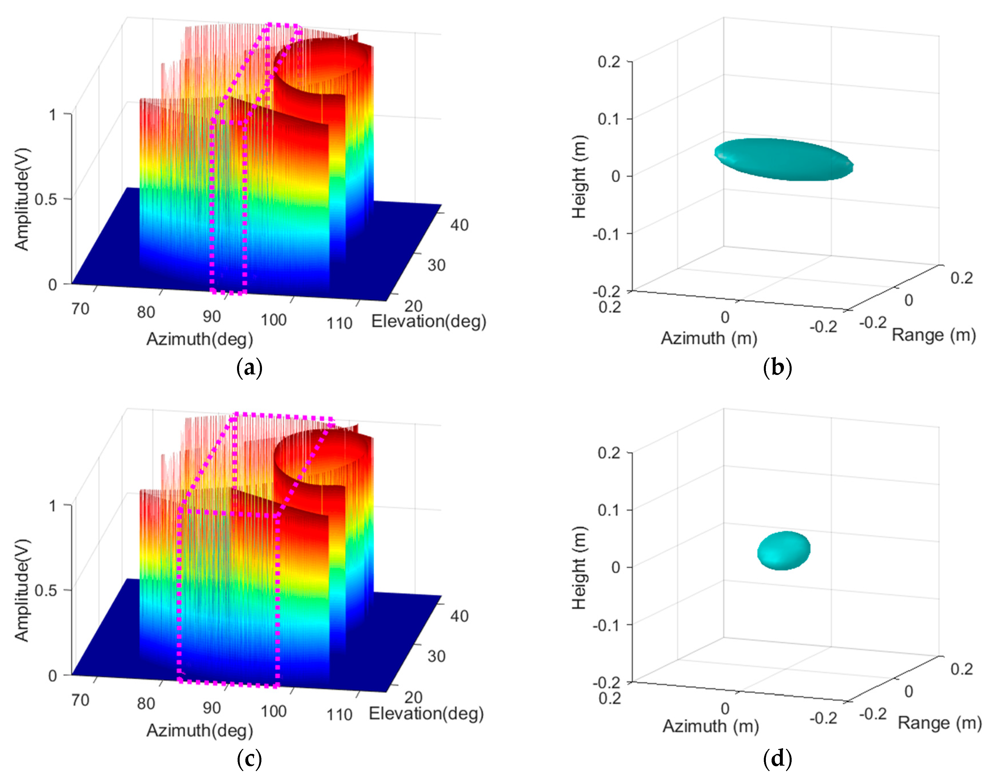
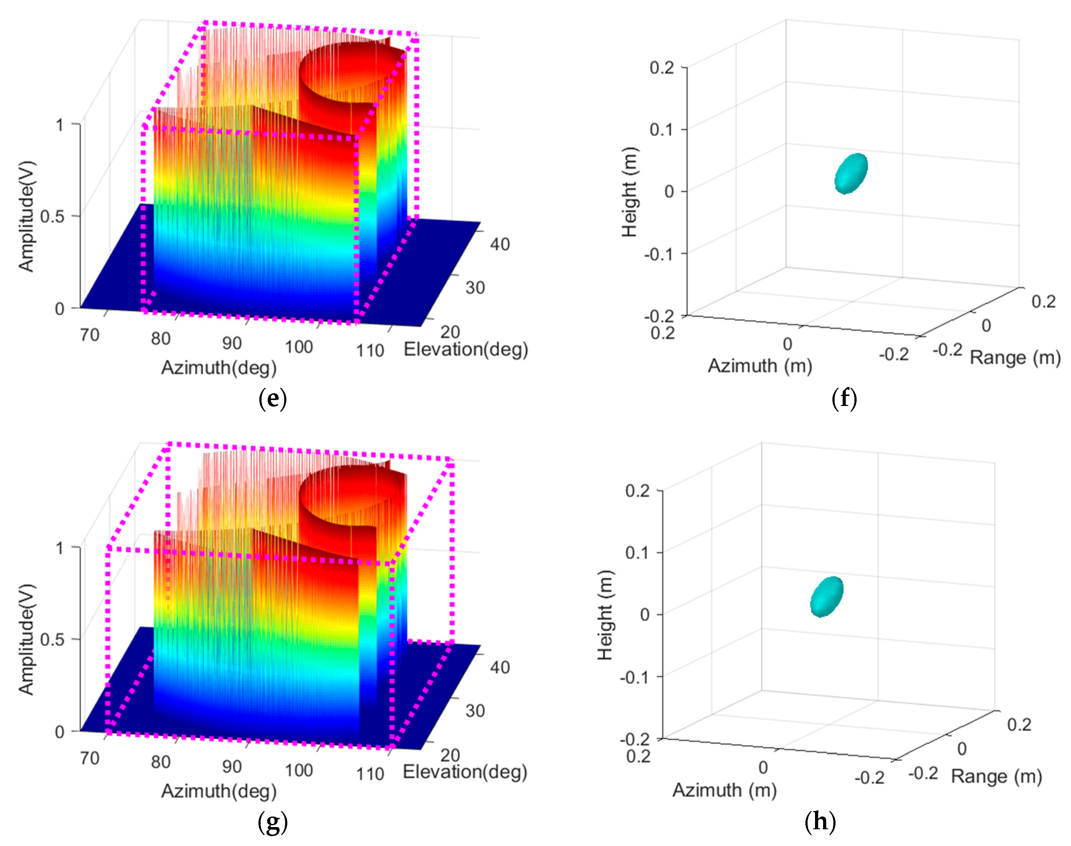
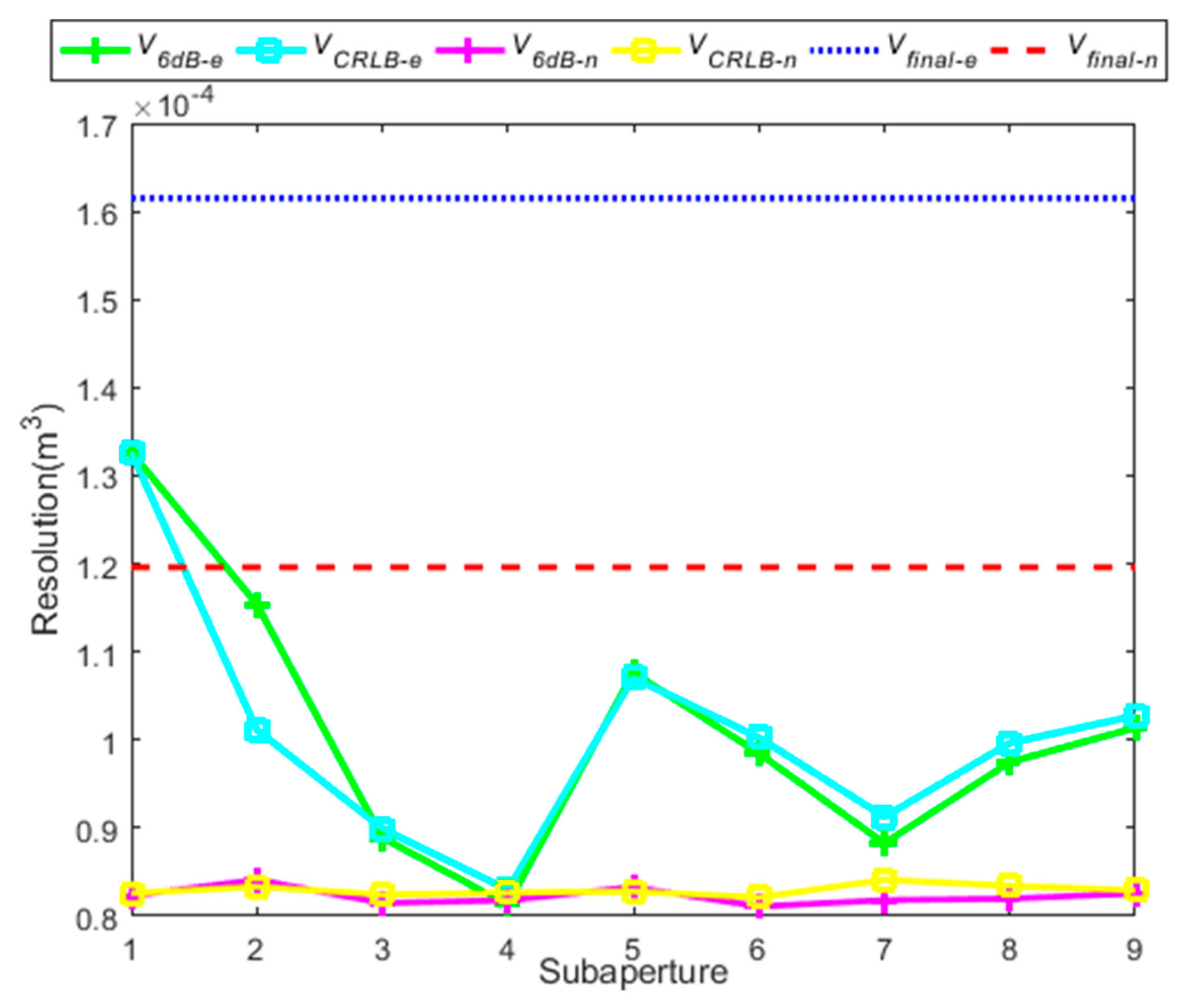
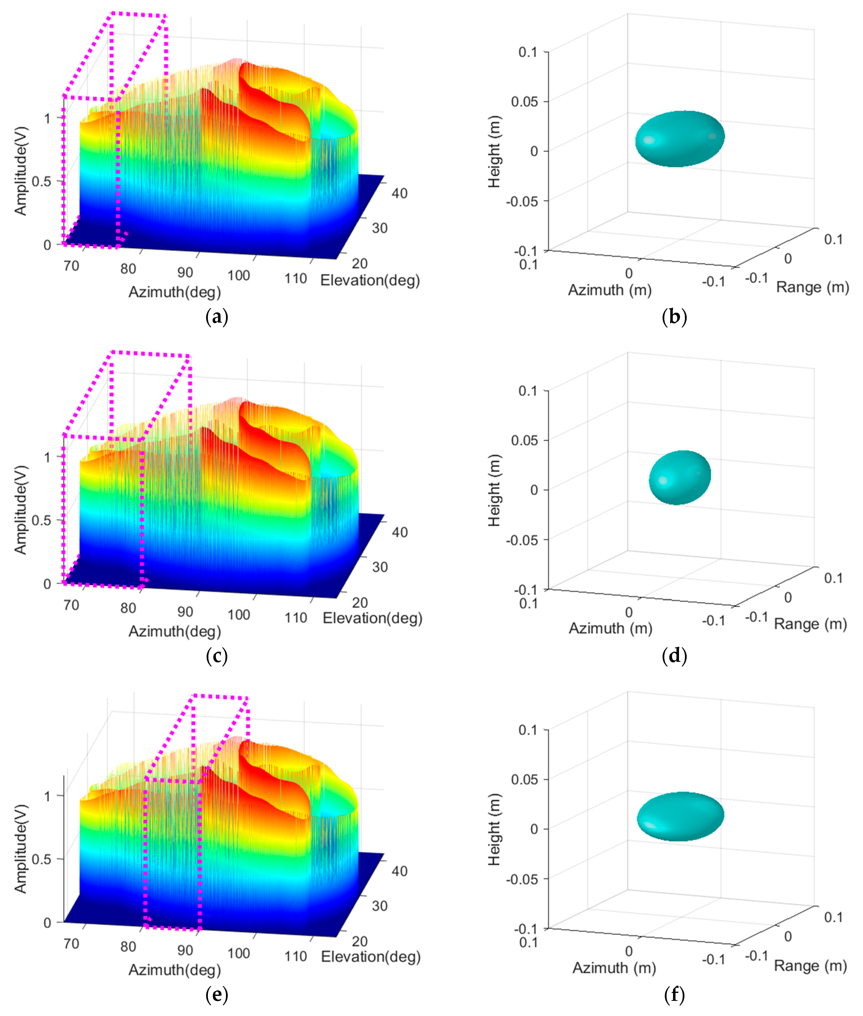
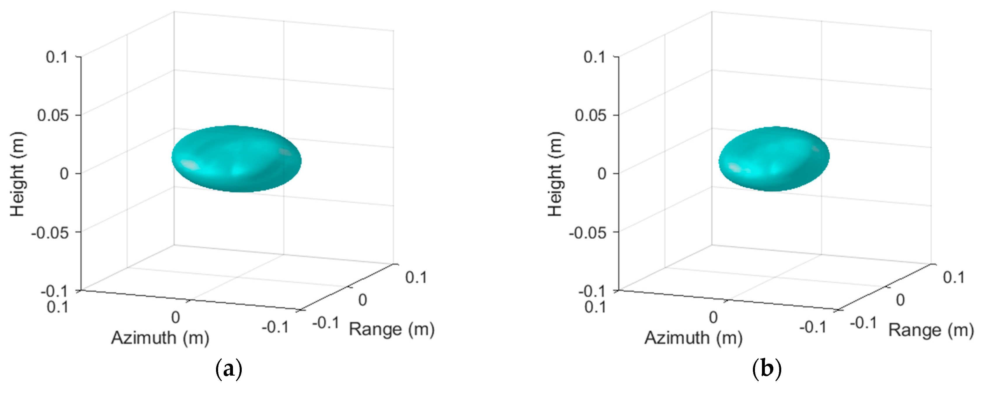
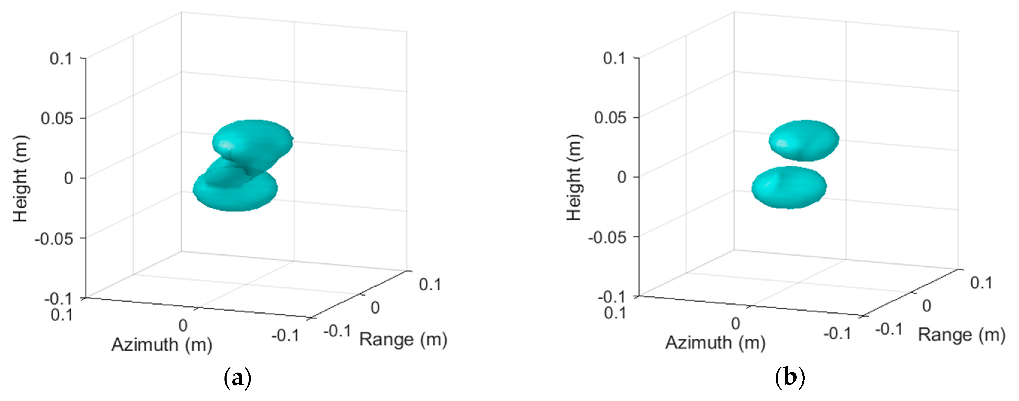
6.1. Estimation of the 3-D Resolution

The correctness of the 3-D resolution estimation V C R L B was verified by the following experiment: A reflector with limited persistence of 30° was placed in the center of the scene. The center frequency of the radar was 10 GHz, and the bandwidth was 2 GHz. The scanning trajectory of radar along elevation and azimuth was consistent with that of five UAVs in cooperative flight shown in Figure 1, and Figure 2b showed its non-uniform K-space sampling. The azimuth and elevation range were [66°, 114°] and [18°, 42°], respectively. The data was simulated by MATLAB through Equation (1).
A comparison of the 3-D resolution estimation V C R L B and the actual 3-D resolution V 6 d B as aperture extent increased is shown in Figure 4. The target was imaged by 3-D NUFFT with the azimuth aperture extent increasing from 5° to 40°. According to the distribution of K-space sampling within the selected aperture, the 3-D resolution estimation V C R L B of the target was calculated by Equation (11). According to the 3-D imaging result, the actual 3-D resolution V 6 d B was represented by the volume of the ellipsoid, which was larger than −6dB in the imaging result. It can be seen from Figure 4 that the trend of the two curves was basically the same, which verified the validity of Equation (11). Furthermore, when the aperture extent was smaller than the persistence of the target (30°), with the increase of the azimuth aperture extent, the better the resolution was, as shown in Figure 4. However, the resolution of the imaging result did not improve when the aperture extent was larger than 30°, since increasing the aperture extent does not bring any useful information. Seen from Figure 4, the two curves tended to be stable when the aperture extent was larger than 30°. In summary, the 3-D resolution was indeed determined by the distribution of K-space sampling and the scattering persistence of the target, as expected in Equation (11).
Specially, Figure 5 gives the target scattering amplitudes and the 3-D imaging results with different aperture extents. The parts within the magenta dotted lines in Figure 5a,c,e,g represent the target scattering amplitudes versus azimuth and elevation with azimuth aperture extent of 5, 15, 30 and 40°, respectively. Additionally, Figure 5a,c,e,g shows the corresponding 3-D imaging results. Consistent with the result shown in Figure 4, the ellipsoid in Figure 5b was larger than in Figure 5d, while the ellipsoid in Figure 5f was the smallest. In addition, the 3-D imaging result with aperture extent of 30° was nearly the same as that of 40°, as shown in Figure 5f,h.

6.2. Performance of the Proposed Sub-Aperture Partitioning Method

The effectiveness of the sub-aperture partitioning method proposed in this paper was verified by two experiments, and both cases were considered– based on a single target and based on two adjacent targets.
A trihedral was placed in the scene, and its 3-D CAD model is shown in Figure 6. The center frequency of radar was 10 GHz, and the bandwidth was 2 GHz. The scanning trajectory of radar along elevation and azimuth was consistent with that of five UAVs in cooperative flight shown in Figure 1, and Figure 2b showed its non-uniform K-space sampling. The azimuth and elevation range were [66°, 114°] and [18°, 42°], respectively. The data were generated by CST Microwave Studio software.
Figure 7 gives the result of sub-aperture partitioning. The number 1 to 9 in Figure 7 represents the sequence number of the current sub-aperture. The azimuth aperture size was 48° for the scene that the azimuth range was [66°, 114°]. When using the equal-interval partitioning method, the aperture of 48° was divided into 9 sub-apertures with equal interval, thus the size of each sub-aperture was 9.6° and the overlapping between each sub-aperture was 4.8°, as shown in Figure 7a. Furthermore, on the basis of the K-space sampling shown in Figure 2b and the number of sub-apertures, the aperture was divided non-uniformly using the method proposed in Section 5. The result of the non-uniform sub-aperture partitioning is shown in Figure 7b.
The resolution comparison of imaging results using different sub-aperture partitioning methods is shown in Figure 8. Firstly, according to the two sub-aperture partitioning results shown in Figure 7, the trihedral is imaged by 3-D NUFFT on each sub-aperture. V 6 d B e and V C R L B e represent the actual 3-D resolution and the 3-D resolution estimation of each sub-aperture obtained by the equal-interval sub-aperture partitioning method, respectively. V 6 d B n and V C R L B n represent the actual 3-D resolution and the 3-D resolution estimation of each sub-aperture obtained by the non-uniform sub-aperture partitioning method, respectively. Specially, V C R L B is calculated by Equation (11) and V 6 d B is represented by the volume of the ellipsoid which is larger than -6dB in the imaging result. Subsequently, the sub-images were combined to reconstruct the final imaging results by the GLRT approach. V f i n a l e and V f i n a l n represent the actual 3-D resolution of the final imaging result obtained by the equal-interval and the non-uniform sub-aperture partitioning method, respectively.
It can be seen from Figure 8 that the trend of V 6 d B e was basically consistent with V C R L B e , also, the trend of V 6 d B n and V C R L B n were basically the same, which verified the validity of Equation (11). In addition, when using the equal-interval sub-aperture partitioning method, the resolution of each sub-aperture varied greatly since V C R L B e and V 6 d B e in Figure 8 obviously fluctuated. On the contrary, for the non-uniform sub-aperture partitioning method, the resolution of each sub-aperture was basically the same as V C R L B n and V 6 d B n in Figure 8. Moreover, V C R L B n and V 6 d B n were always below V C R L B e and V 6 d B e , which meant that the resolution of each sub-aperture obtained by the non-uniform sub-aperture partitioning method was better than that obtained by the equal-interval sub-aperture partitioning method. Although the size of each sub-aperture was the same in the equal-interval method, the resolution of each sub-aperture was obviously different due to the different distributions of K-space sampling in each sub-aperture. However, considering the distribution of K-space sampling in each sub-aperture, the proposed method ensured that the resolution of each sub-aperture was consistent and high. Finally, V f i n a l n was much lower than V f i n a l e , which indicated that the resolution of the final 3-D imaging result after the non-uniform sub-aperture partitioning outperformed that after the equal-interval sub-aperture partitioning. As a matter of fact, the resolution of the final imaging result was determined by the sub-image with the worst resolution. When using the equal-interval sub-aperture partitioning method, the resolution of the first sub-aperture was very poor, which resulted in poor resolution of the final imaging result. However, for non-uniform sub-aperture partitioning, since the resolution of each sub-image was consistent and high, a high-resolution imaging result was obtained.
Specially, the target scattering amplitudes and the 3-D imaging results of different sub-apertures obtained by different sub-aperture partitioning methods are shown in Figure 9. The parts within the magenta dotted lines in Figure 9a,e represents the target scattering amplitudes within sub-aperture 1 and sub-aperture 4 obtained by the equal-interval sub-aperture partitioning method, respectively. Additionally, Figure 9b,f shows the corresponding 3-D imaging results. The parts within the magenta dotted lines in Figure 9c,g represents the target scattering amplitudes within sub-aperture 1 and sub-aperture 4 obtained by the non-uniform sub-aperture partitioning method, respectively. Figure 9d,h shows the corresponding 3-D imaging results. Because the extent of elevation was 24° while the extent of azimuth was only about 10°, the elevation resolution was finer than the azimuth resolution, which made the imaging result in Figure 9 ellipsoid. Consistent with the result shown in Figure 8, the ellipsoid in Figure 9b was larger than that in Figure 9f. The resolution of each sub-aperture was obviously different when using the equal-interval method. For the reason that the resolution of sub-aperture 1 was the worst, while that of sub-aperture 4 was the best in the equal-interval method, the proposed non-uniform sub-aperture partitioning method adjusted the size of each new sub-aperture until the resolution of each new sub-aperture was the same as the sub-aperture 4 in the equal-interval method. Therefore, the ellipsoid in Figure 9d was smaller than that in Figure 9b, and the ellipsoid in Figure 9f was basically the same as that in Figure 9h, which was consistent with the result shown in Figure 8.
Figure 10 gives the final 3-D imaging result of the trihedral. Figure 10a,b was obtained by the equal-interval and the non-uniform sub-aperture partitioning method, respectively. Consistent with the result shown in Figure 8, the ellipsoid in Figure 10a was larger than that in Figure 10b. In summary, the resolution of imaging result was improved by using the non-uniform sub-aperture partitioning method proposed in this paper.
Two adjacent trihedrals were placed in the scene, and its 3-D CAD model is shown in Figure 11. The center frequency of the radar was 10 GHz, and the bandwidth was 2 GHz. The scanning trajectory of radar along elevation and azimuth was consistent with that of five UAVs in cooperative flight shown in Figure 1, and Figure 2b showed its non-uniform K-space sampling. The azimuth and elevation range were [66°, 114°] and [18°, 42°], respectively. The data were generated by CST Microwave Studio software.
The final 3-D imaging result of two adjacent trihedral is shown in Figure 12. Figure 12a,b was obtained by the equal-interval and the non-uniform sub-aperture partitioning method, respectively. As can be seen in Figure 12, two adjacent trihedrals were not distinguished in Figure 12a, but were distinguished in Figure 12b. The imaging result in Figure 12b had a better resolution than that in Figure 12a. Therefore, using the equal-interval sub-aperture partitioning method for non-uniformly sampled SAR may cause a mismatch between the imaging result and the real scene. However, a higher resolution imaging result can be obtained by the non-uniform sub-aperture partitioning method, compared with the equal-interval method. In summary, the theoretical analysis and simulation results verify the feasibility and effectiveness of the proposed method in this paper.

7. Conclusions

For 3-D wide-angle SAR with non-uniform sampling, dividing the aperture with equal intervals has a bad influence on the resolution of the SAR imaging result. In this paper, the sub-aperture partitioning problem under non-uniform sampling was studied for the first time and a non-uniform sub-aperture partitioning method was proposed. According to the relationship between the 3-D resolution and the sampling distribution in K-space, the proposed method searched the optimum size of each sub-aperture and the aperture was divided non-uniformly. Since the proposed method ensured that the resolution of each sub-aperture was consistent and high, the resolution of the final imaging result obtained by the proposed method was much better than that by the equal-interval sub-aperture partitioning method. The effectiveness of the proposed method was verified by using electromagnetic simulation data.
Combining sparse imaging with the proposed method may improve imaging quality and resolution of the imaging result. In addition, the proposed method in this paper can also image complex targets. These interesting problems will be further studied in future.

Author Contributions

D.S. and S.X. designed the algorithm; D.S. and Y.L. performed the algorithm; S.X. and B.P. proposed an important modified scheme of the paper; D.S. wrote the paper; X.W. revised the paper.

Funding

This research was funded by the National Natural Science Foundation of China (No. 61490692, 61490693).

Acknowledgments

The authors wish to extend their sincere thanks to Yi Zhang ([email protected]) for her careful reading and fruitful suggestions.

Conflicts of Interest

The authors declare no conflicts of interest.

References

  1. Xu, F.; Jin, Y.Q.; Moreira, A. A Preliminary Study on SAR Advanced Information Retrieval and Scene Reconstruction. IEEE Geosci. Remote Sens. Lett. 2016, 13, 1443–1447. [Google Scholar] [CrossRef]
  2. CongHui, M.; GongJian, W.; XiaoHong, H.; XiaoLiang, Y.; BaiYuan, D. Scatterer-based approach to evaluate similarity between 3D em-model and 2D SAR data for ATR. IET Radar Sonar Navig. 2016, 11, 254–259. [Google Scholar] [CrossRef]
  3. Song, H.; Ji, K.; Zhang, Y.; Xing, X.; Zou, H. Sparse Representation-Based SAR Image Target Classification on the 10-Class MSTAR Data Set. Appl. Sci. 2016, 6, 26. [Google Scholar] [CrossRef]
  4. Reigber, A.; Lombardini, F.; Viviani, F.; Nannini, M.; Martinez Del Hoyo, A. Three-dimensional and higher-order imaging with tomographic SAR: Techniques, applications, issues. In Proceedings of the 2015 IEEE International Geoscience and Remote Sensing Symposium (IGARSS), Milan, Italy, 26–31 July 2015. [Google Scholar]
  5. Wang, X.; Xu, F.; Jin, Y.Q. The Iterative Reweighted Alternating Direction Method of Multipliers for Separating Structural Layovers in SAR Tomography. IEEE Geosci. Remote Sens. Lett. 2017, 14, 1883–1887. [Google Scholar] [CrossRef]
  6. Ponce, O.; Prats-Iraola, P.; Pinheiro, M.; Rodriguez-Cassola, M.; Scheiber, R.; Reigber, A.; Moreira, A. Fully polarimetric high-resolution 3-D imaging with circular SAR at L-band. IEEE Trans. Geosci. Remote Sens. 2014, 52, 3074–3090. [Google Scholar] [CrossRef]
  7. Varshney, K.R.; Çetin, M.; Fisher III, J.W.; Willsky, A.S. Joint image formation and anisotropy characterization in wide-angle SAR. Algorithms Synth. Aperture Radar Imag. XIII 2006, 6237, 62370D. [Google Scholar]
  8. Gao, Y.; Xing, M. A method for extracting amplitude attribute of scattering centers in SAR. In Proceedings of the IEEE International Geoscience and Remote Sensing Symposium (IGARSS), Beijing, China, 10–15 July 2016; pp. 2665–2668. [Google Scholar]
  9. Austin, C.D.; Ertin, E.; Moses, R.L. Sparse signal methods for 3-D radar imaging. IEEE J. Sel. Top. Signal Process. 2011, 5, 408–423. [Google Scholar] [CrossRef]
  10. Liu, D.; Boufounos, P.T. Compressive sensing based 3D SAR imaging with multi-PRF baselines. In Proceedings of the IEEE Geoscience and Remote Sensing Symposium, Quebec City, QC, Canada, 13–18 July 2014; pp. 1301–1304. [Google Scholar]
  11. Frey, O.; Magnard, C.; Rüegg, M.; Meier, E. Focusing of airborne synthetic aperture radar data from highly nonlinear flight tracks. IEEE Trans. Geosci. Remote Sens. 2009, 47, 1844–1858. [Google Scholar] [CrossRef]
  12. Axelsson, S.R.J. Beam characteristics of three-dimensional SAR in curved or random paths. IEEE Trans. Geosci. Remote Sens. 2004, 42, 2324–2334. [Google Scholar] [CrossRef]
  13. Zhang, S.; Zhu, Y.; Dong, G. Gangyao Kuang Truncated SVD-Based Compressive Sensing for Downward-Looking Three-Dimensional SAR Imaging With Uniform/Nonuniform Linear Array. IEEE Geosci. Remote Sens. Lett. 2015, 12, 1853–1857. [Google Scholar] [CrossRef]
  14. Aguasca, A.; Acevo-Herrera, R.; Broquetas, A.; Mallorqui, J.J.; Fabregas, X. ARBRES: Light-weight CW/FM SAR sensors for small UAVs. Sensors 2013, 13, 3204–3216. [Google Scholar] [CrossRef] [PubMed]
  15. Lort, M.; Aguasca, A.; López-Martínez, C.; Marín, T.M. Initial evaluation of SAR capabilities in UAV multicopter platforms. IEEE J. Sel. Top. Appl. Earth Obs. Remote Sens. 2018, 11, 127–140. [Google Scholar] [CrossRef]
  16. Li, J.; Chen, J.; Wang, P.; Li, C. Sensor-oriented path planning for multiregion surveillance with a single lightweight UAV SAR. Sensors 2018, 18, 548. [Google Scholar] [CrossRef]
  17. Ash, J.; Ertin, E.; Potter, L.C.; Zelnio, E. Wide-angle synthetic aperture radar imaging: Models and algorithms for anisotropic scattering. IEEE Signal Process. Mag. 2014, 31, 16–26. [Google Scholar] [CrossRef]
  18. Jackson, J.A.; Rigling, B.D.; Moses, R.L. Canonical scattering feature models for 3D and bistatic SAR. IEEE Trans. Aerosp. Electron. Syst. 2010, 46, 525–541. [Google Scholar] [CrossRef]
  19. Stojanovic, I.; Cetin, M.; Karl, W.C. Joint space aspect reconstruction of wide-angle SAR exploiting sparsity. Algorithms Synth. Aperture Radar Imag. XV 2008, 6970, 697005. [Google Scholar]
  20. Sun, C.; Wang, B.; Fang, Y.; Song, Z.; Wang, S. Multichannel and wide-angle SAR imaging based on compressed sensing. Sensors 2017, 17, 295. [Google Scholar] [CrossRef]
  21. Xue, F.; Lin, Y.; Hong, W.; Yin, Q.; Zhang, B.; Shen, W.; Zhao, Y. Analysis of azimuthal variations using multi-aperture polarimetric entropy with circular SAR images. Remote Sens. 2018, 10, 123. [Google Scholar] [CrossRef]
  22. Moore, L.; Potter, L.; Ash, J. Three-dimensional position accuracy in circular synthetic aperture radar. IEEE Aerosp. Electron. Syst. Mag. 2014, 29, 29–40. [Google Scholar] [CrossRef]
  23. Sengijpta, S.K. Fundamentals of Statistical Signal Processing: Estimation Theory. Technometrics 1995, 37, 465–466. [Google Scholar] [CrossRef]
  24. Parker, J.T.; Moore, L.J.; Potter, L.C. Resolution and Sidelobe Structure Analysis for RF Tomography. In Proceedings of the IEEE RadarCon (RADAR), Kansas City, MO, USA, 23–27 May 2011; pp. 1080–1085. [Google Scholar]
Figure 1. The flight trajectory of Tomo-SAR and five UAVs with SAR system in cooperative flight.
Electronics 08 00629 g001
Figure 2. The K-space sampling of Tomo-SAR and five UAVs with SAR system in cooperative flight. (a) Tomo-SAR; (b) five UAVs with SAR system in cooperative flight.
Electronics 08 00629 g002
Figure 3. The flowchart of the non-uniform sub-aperture partitioning method.
Electronics 08 00629 g003
Figure 4. 3-D resolution versus azimuth aperture extent.
Electronics 08 00629 g004
Figure 5. Target scattering amplitudes and 3-D imaging results with different azimuth aperture extents. (a,c,e,g) show target scattering amplitudes with azimuth aperture extent of 5, 15, 30 and 40°, respectively; (b,d,f,h) show 3-D imaging results with azimuth aperture extent of 5, 15, 30 and 40°, respectively.
Electronics 08 00629 g005aElectronics 08 00629 g005b
Figure 6. 3-D CAD model of the trihedral.
Electronics 08 00629 g006
Figure 7. Result of sub-aperture partitioning. (a) Equal-interval; (b) non-uniform.
Electronics 08 00629 g007
Figure 8. Resolution comparison of imaging results using different sub-aperture partitioning methods.
Electronics 08 00629 g008
Figure 9. Target scattering amplitudes and 3-D imaging results of different sub-apertures obtained by different sub-aperture partitioning methods. (a,e) and (b,f) show target scattering amplitudes and 3-D imaging results of sub-aperture 1 and sub-aperture 4 obtained by the equal-interval sub-aperture partitioning method, respectively; (c,g) and (d,h) show target scattering amplitudes and 3-D imaging results of sub-aperture 1 and sub-aperture 4 obtained by the non-uniform sub-aperture partitioning method, respectively.
Electronics 08 00629 g009aElectronics 08 00629 g009b
Figure 10. Final 3-D imaging result of the trihedral. (a) Equal-interval; (b) non-uniform.
Electronics 08 00629 g010
Figure 11. 3-D CAD model of two adjacent trihedral.
Electronics 08 00629 g011
Figure 12. Final 3-D imaging result of two adjacent trihedral. (a) Equal-interval; (b) non-uniform.
Electronics 08 00629 g012
Table 1. The steps for the non-uniform sub-aperture partitioning method.
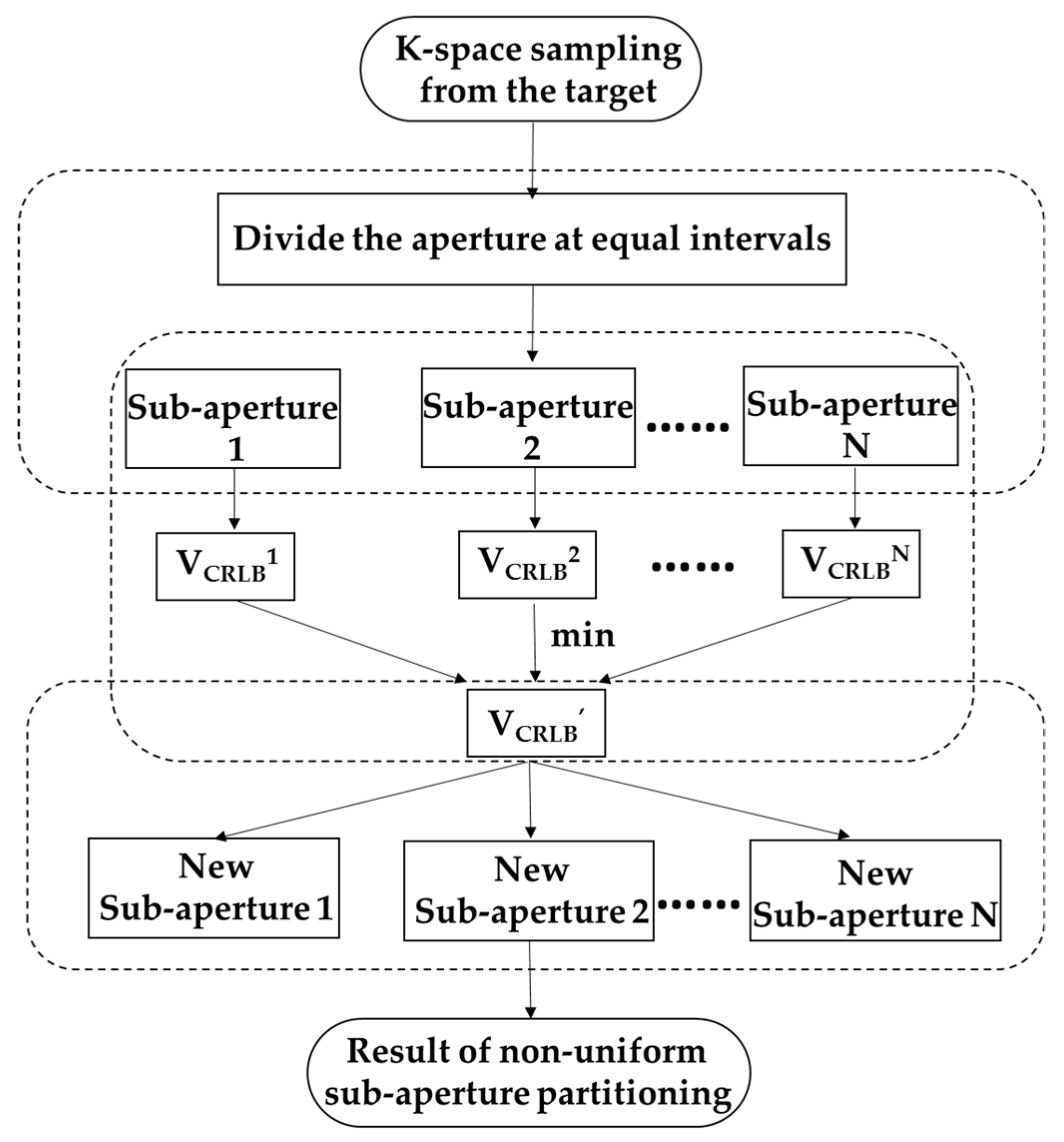
The Non-Uniform Sub-Aperture Partitioning Method
1.
Input: sub-aperture number n , azimuth original angle θ 1 , azimuth terminate angle θ 2 .
2.
Divide the aperture with equal intervals θ o = 2 ( θ 2 θ 1 ) n + 1 , the azimuth range of the i t h sub-aperture ( θ c i , θ l i ) is [ θ 1 + i 1 2 θ 0 , θ 1 + i + 1 2 θ 0 ] .
3.
Calculate V C R L B ( θ c i , θ l i ) of the i t h sub-aperture ( θ c i , θ l i ) by Equation (11), find the minimum value V C R L B = min i ( V C R L B ( θ c i , θ l i ) ) .
4.
Search the optimum size of the first new sub-aperture ( θ ˜ c 1 , θ ˜ l 1 ) so that V C R L B ( θ ˜ c 1 , θ ˜ l 1 ) = V C R L B , the values of θ ˜ c 1 and θ ˜ l 1 are obtained by the relationship θ ˜ c 1 1 2 θ ˜ l 1 = θ 1 .
5.
Search the optimum size of the last new sub-aperture ( θ ˜ c n , θ ˜ l n ) so that V C R L B ( θ ˜ c n , θ ˜ l n ) = V C R L B , the values of θ ˜ c n and θ ˜ l n are obtained by the relationship θ ˜ c n + 1 2 θ ˜ l n = θ 2 .
6.
Deduce the azimuthal central angle θ ˜ c i of the i ( 1 < i < n ) t h new sub-aperture, and obtain θ ˜ c i = θ 1 + θ ˜ l 1 2 + ( i 1 ) θ 2 θ 1 θ ˜ l 1 / 2 θ ˜ l n / 2 n 1 .
7.
Search the optimum size of the i ( 1 < i < n ) t h new sub-aperture ( θ ˜ c i , θ ˜ l i ) so that V C R L B ( θ ˜ c i , θ ˜ l i ) = V C R L B , the value of θ ˜ l i is obtained according to the known θ ˜ c i .
8.
Output: Non-uniform sub-aperture partitioning result ( θ ˜ c i , θ ˜ l i ) .

