Model Predictive Current Control Method with Improved Performances for Three-Phase Voltage Source Inverters

Abstract

In this paper, the model predictive current control (MPCC) method using two vectors has been proposed to control output currents of three-phase voltage source inverters (VSIs) with small current errors and current ripples. Also, the proposed method can reduce switching losses by applying the vector pre-selection technique to the MPCC for the VSI. The VSI generates seven voltage vectors to control the output currents, but the proposed method uses four available voltage vectors with one switch, which are classified by the vector pre-selection method clamping one leg and conducting the largest output current among the three legs to reduce the switching losses. In the proposed method, selecting two future voltage vectors among the four voltage vectors and dividing them in a future sampling period are determined by an optimization process. The proposed method results in the lower total loss, better total harmonic distortion (THD), and smaller current errors than the conventional method with half the sampling period of the proposed method due to the optimal process. Simulation and experimental results of the three-phase VSIs are presented in order to verify the effectiveness of the proposed method.

1. Introduction

In the last few decades, the control schemes for voltage source inverters (VSIs) have been presented and widely studied [1,2].The typical control schemes for voltage source inverter are hysteresis control and linear control with pulse width modulation (PWM). New control schemes, such as fuzzy logic control, neural networks, and predictive control, have been proposed due to the improvement of fast and powerful microprocessors. Among the new control schemes, model predictive control (MPC) using a finite-control-set is simple and effective for VSIs because it is simple and flexible without any PWM blocks [3,4,5]. Thanks to its simplicity and control flexibility, the MPC has been used in power electronics for VSIs, including active front ends [6,7,8], multi-level inverters [9,10,11,12], and matrix converters [13,14,15]. The VSIs can be controlled by using the model predictive control, which predicts the finite number of the future output current behaviors based on the load dynamic model. A cost function with respect to the error term between the predicted current and reference current is used to evaluate all predicted current values obtained by possible switching states to select one optimal switching state with the smallest cost value [16,17,18,19]. The optimal switching state is applied to the VSIs in one sampling period [20,21]. The conception of using two vectors has also recently been applied in the MPC for the torque control and flux control to reduce torque and flux ripples and the PWM rectifier to reduce power ripples [22]. This paper proposes a switching strategy, that is, the vector pre-selection technique to obtain high efficiency [23], and the model predictive current control method based on using two vectors during one sampling period to reduce current errors and ripples [24,25]. In order to obtain high efficiency, the switching strategy classifies the four available voltage vectors with one switch that clamps one leg carrying the largest current among the three legs in the VSIs. The proposed method selects two vectors among four available vectors classified by pre-selection method by using a cost function defined at the changing point of the two voltage vectors, as well as at the next sampling instants to evaluate the predicted current values. Therefore, the newly defined cost function takes into account current errors at two points, and the proposed method distributes two selected vectors within the sampling period in a manner that minimizes the squared current errors in the cost function. The proposed method leads to lower total loss [26], better current total harmonic distortion (THD), and smaller current errors compared to the model predictive current control (MPCC) method using one vector during one sampling period. Simulation and experimental results of the three-phase VSIs are presented in order to verify the effectiveness of the proposed method.

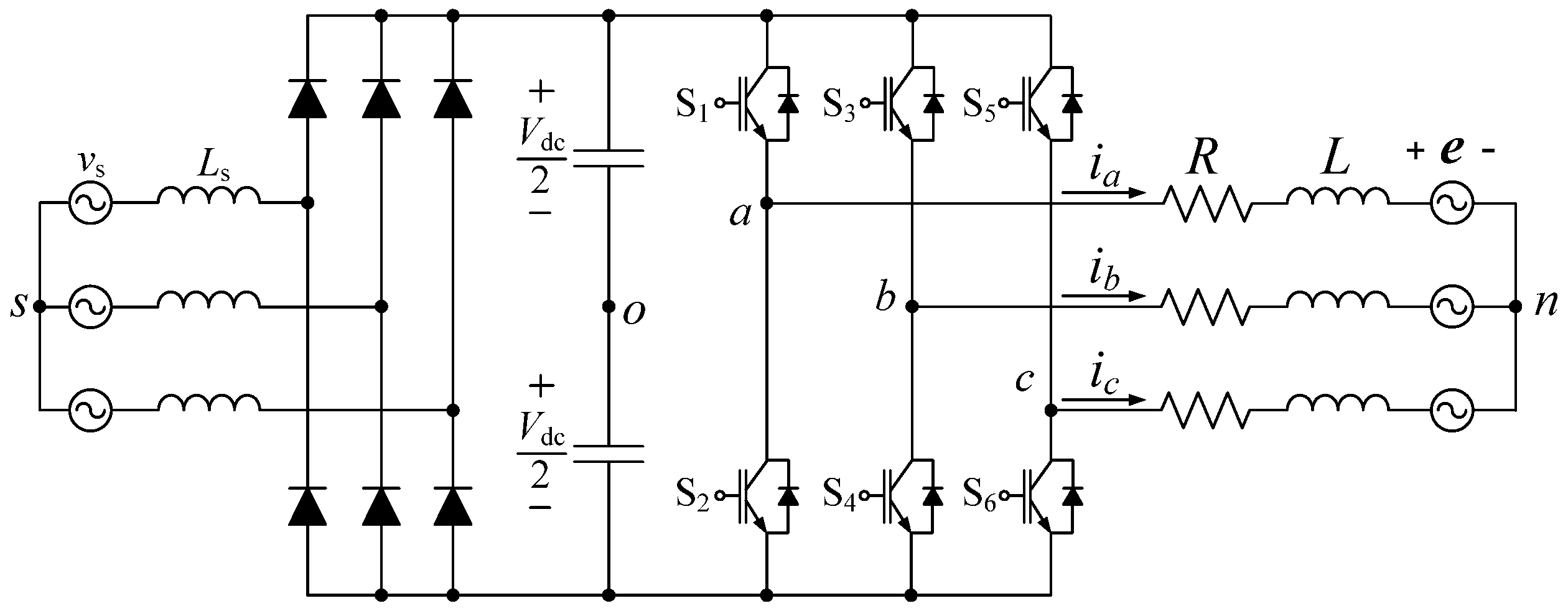
2. Conventional Model Predictive Current Control Method for VSIs

The basic structure of the three-phase VSI is shown in the following Figure 1.

The three-phase VSI has three legs and each of which consists of two switches. The two switches in each leg operate complementary to each other. The output voltage vectors generated by the switches can be expressed as

$$\mathit{v}=\frac{2}{3}\left(v_{an}+v_{bn}{e}^{j\left(2\pi /3\right)}+v_{cn}{e}^{j\left(4\pi /3\right)}\right)$$

(1)

where $v_{an}$, $v_{bn}$, and $v_{cn}$ are the phase-to-neutral voltages.

The three-phase VSI composed of six switches has a total of eight load voltage vectors divided into six active vectors and two zero vectors, as shown in Figure 2, in accordance with a combination of switching states. Since the two zero vectors among eight voltage vectors produce the same output voltage vectors, only seven voltage vectors are considered as control elements. The output current can be also expressed as

$$\mathit{i}=\frac{2}{3}\left(i_a+i_b{e}^{j\left(2\pi /3\right)}+i_c{e}^{j\left(4\pi /3\right)}\right)$$

(2)

where $i_a$, $i_{b,}$ and $i_c$ are the three-phase output currents. The output current dynamics can be described by the differential equation as

$$\mathit{v}=R\mathit{i}+L\frac{d\mathit{i}}{dt}+\mathit{e}$$

(3)

where v, i, R, L, and e are the voltage vectors produced by the VSI, the output current vector, the load resistance, inductance, and load back-emf vector, respectively. The output current derivative di/dt in (3) can be replaced by the Forward Euler approximation with a sampling period T_s as

$$\frac{d\mathit{i}}{dt}\approx \frac{\mathit{i}\left(k+1\right)-\mathit{i}\left(k\right)}{T_s}$$

(4)

Then, the output current at the next sampling period can be expressed as

$$\mathit{i}\left(k+1\right)=\mathit{i}\left(k\right)+\frac{T_s}{L}\left[{\mathit{v}}^k-R\mathit{i}\left(k\right)-\mathit{e}\left(k\right)\right]$$

(5)

Seven future output currents generated by the seven voltage vectors ${\mathit{v}}^k$ in the k^th sampling period can be predicted by using (5). A predefined cost function composed of errors between the future output currents and the future reference currents is used to select the optimal vector among seven available voltage vectors minimizing the errors at every sampling period. The two-step future output current at the (k + 2)^th instant is obtained by shifting (5) one step forward as in [2] to prevent the unavoidable calculation delay,

$$\mathit{i}\left(k+2\right)=\mathit{i}\left(k+1\right)+\frac{T_s}{L}\left[{\mathit{v}}^{k+1}-R\mathit{i}\left(k+1\right)-\mathit{e}\left(k+1\right)\right]$$

(6)

Thus, the cost function considering calculation delay can be defined as the second order errors as

$$g={\{i_{\alpha }^{\ast }\left(k+2\right)-i_{\alpha }\left(k+2\right)\}}^2+{\{i_{\beta }^{\ast }\left(k+2\right)-i_{\beta }\left(k+2\right)\}}^2$$

(7)

where i and i^* are the output current and the reference output current in the αβ frame, respectively. The future reference current value required in the cost function can be obtained by the Lagrange extrapolation formula as

$${\mathit{i}}^{\ast }\left(k+2\right)=3{\mathit{i}}^{\ast }\left(k+1\right)-3{\mathit{i}}^{\ast }\left(k\right)+{\mathit{i}}^{\ast }\left(k-1\right)$$

(8)

The back-emf vector in (6) can be estimated by assuming that the future back-emf vector is equal to the present back-emf vector because the back-emf vector varies at a much lower frequency compared with the fast sampling frequency. The present back-emf vector can be calculated from (5) as

$$\mathit{e}\left(k+1\right)\approx \mathit{e}\left(k\right)={\mathit{v}}^k-R\mathit{i}\left(k\right)-\frac{L}{T_s}\left[\mathit{i}\left(k+1\right)-\mathit{i}\left(k\right)\right]$$

(9)

Only one voltage vector selected from the seven possible voltage vectors is applied for one full sampling period. Thus, the conventional method uses the optimal voltage vector that minimizes the current error, and the vector is maintained for at least one sampling period.

3. Proposed Model Predictive Current Control Method to Improve Performance in Terms of Efficiency and Current Harmonics

The instantaneous switching losses of the VSI depend on the amplitude of the output currents through the switches at the moment of switching. Thus, the vector pre-selection method sorts the voltage vectors clamping one leg and carrying the largest current among the three legs to reduce the switching losses. In order to sort the voltage vectors among the seven voltage vectors of the VSI, the inverse model equation in (10) is used to obtain the future reference voltage vector at (k + 1)^th sampling instant.

$${\mathit{v}}^{k+1}=\frac{L}{T_s}\left\{\mathit{i}\left(k+2\right)-\left(1-\frac{R{T}_s}{L}\right)\mathit{i}\left(k+1\right)\right\}+\mathit{e}\left(k+1\right)$$

(10)

In the inverse model equation, the output currents are replaced with the reference currents to reduce ripples of the future reference voltage vector. The vector pre-selection method selects the voltage vectors in accordance with the state of the future output currents and phase voltages at every sampling period. The three-phase future voltages obtained by using (10) are classified as ${\mathit{v}}_{max}^{k+1}$, ${\mathit{v}}_{mid}^{k+1}$, and ${\mathit{v}}_{min}^{k+1}$ according to the magnitude of each phase future voltage and are assigned as

$$\begin{array}{c}{\mathit{v}}_{max}^{k+1}=\max \left({\mathit{v}}_a^{k+1},{\mathit{v}}_b^{k+1},{\mathit{v}}_c^{k+1}\right)\\ {\mathit{v}}_{mid}^{k+1}=\mathrm{mid}\left({\mathit{v}}_a^{k+1},{\mathit{v}}_b^{k+1},{\mathit{v}}_c^{k+1}\right)\\ {\mathit{v}}_{min}^{k+1}=\min \left({\mathit{v}}_a^{k+1},{\mathit{v}}_b^{k+1},{\mathit{v}}_c^{k+1}\right)\end{array}$$

(11)

The prohibitive phase that should not be allowed to be clamped corresponds with the phase with the future voltage ${\mathit{v}}_{mid}^{k+1}$, that is, the medium value among the three-phase future voltage to assure linear modulation ranges. In the two voltages classified as ${\mathit{v}}_{max}^{k+1}$ and ${\mathit{v}}_{min}^{k+1}$, the future reference currents determine that one phase with a higher absolute output current is clamped to the positive or negative DC-link. Once it is determined that one leg of the VSIs is clamped, the upper switch or the lower switch is compelled to turn on according to the sign of the corresponding reference voltage. Figure 3 shows pre-selected vectors and the clamped switches according to the output currents and phase voltages. Four voltage vectors among seven voltage vectors can clamp one phase exposed to the higher output current between two voltages classified as ${\mathit{v}}_{max}^{k+1}$ and ${\mathit{v}}_{min}^{k+1}$, so the four available voltage vectors can be pre-selected.

Table 1. Conditions of the vector pre-selection.

Conditions				Pre-Selected Vectors		Clamped Switch
Phase Voltages		Output Currents
Max	Min	Max	Min	Active	Zero
van	vcn	ia	ib	V1V2V6	V7	S1
vcn	van	ib	ia	V3V4V5	V0	S2
vbn	van	ib	ic	V2V3V4	V7	S3
van	vbn	ic	ib	V1V5V6	V0	S4
vcn	vbn	ic	ia	V4V5V6	V7	S5
vbn	vcn	ia	ic	V1V2V3	V0	S6

shows the clamped switches, pre-selected vectors, and the conditions of the output currents and phase voltages, making switches clamping. The proposed method uses two vectors among the four available voltage vectors for reducing the output current errors and ripples. Optimal two voltage vectors and their optimal durations have to be selected to generate the output current closely tracking the reference current because of using the two vectors in one sampling period. In this paper, the proposed method using two vectors is proposed to reduce switching losses, current errors, and current ripples.

In order to reduce output current errors and ripples, the proposed method uses two vectors defined as the initial and the next voltage vector at every sampling point. The two vectors are divided by the optimization process in a sampling period. The selected voltage vectors in the proposed method are applied for the calculation of the cost function minimizing the output current errors at every sampling point. One sampling period $T_s$ is divided into the time intervals $T_1^k$ and $T_2^k$ depending on selected voltage vectors at every sampling point, as

$$T_s=T_1^k+T_2^k$$

(12)

Each of the durations $T_1^k$ and $T_2^k$ has a positive value from 0 to $T_s$ because $T_1^k$ and $T_2^k$ are the time intervals for the initial voltage vector ${\mathit{v}}_1^k$ and the next voltage vector ${\mathit{v}}_2^k$, respectively. In the proposed method, the predicted output current in (5) can be modified as

$$\mathit{i}\left(k+1\right)=\mathit{i}\left(k\right)+\frac{T_1^k}{L}\left[{\mathit{v}}_1^k-R\mathit{i}\left(k\right)-\mathit{e}\left(k\right)\right]+\frac{T_2^k}{L}\left[{\mathit{v}}_2^k-R\mathit{i}\left(k+T_1^k\right)-\mathit{e}\left(k+T_1^k\right)\right]$$

(13)

In the one sampling period, the back-emf vector $e\left(k+T_1^k\right)$ does not change considerably, so it can be estimated as

$$\mathit{e}\left(k\right)\approx \mathit{e}\left(k+T_1^k\right)$$

(14)

The present back-emf is assumed by using an extrapolation of the past value by shifting (10) one-step backward as

$$\begin{array}{l}\mathit{e}\left(k\right)\approx \mathit{e}\left(k-1\right)\\ =\frac{T_1^{k-1}}{T_s}\left[v_1^{k-1}-Ri\left(k-1\right)\right]+\frac{T_2^{k-1}}{T_s}\left[v_2^{k-1}-Ri\left(\left(k-1\right)+T_1^{k-1}\right)\right]-\frac{L}{T_s}[i\left(k\right)-i\left(k-1\right)\end{array}$$

(15)

To prevent the control delay, the two-step future output current can be obtained by shifting (13) one step forward as

$$\begin{array}{ll}\mathit{i}\left(k+2\right)=& \mathit{i}\left(k+1\right)+\frac{T_1^{k+1}}{L}\left[{\mathit{v}}_1^{k+1}-R\mathit{i}\left(k+1\right)-\mathit{e}\left(k+1\right)\right]\\ & +\frac{T_2^{k+1}}{L}\left[{\mathit{v}}_2^{k+1}-R\mathit{i}\left(\left(k+1\right)+T_1^{k+1}\right)-\mathit{e}\left((k+1\right))+T_1^{k+1}\right]\end{array}$$

(16)

In case that the proposed scheme uses the cost function (7), which considers the current errors at next sampling instant, the current errors at changing point of the two vectors could be higher than at the next sampling instant. So, a cost function of the proposed scheme has to contain the output currents at changing point of the two vectors. Therefore, the cost function for the proposed scheme is considered at two instants, as

$$\begin{array}{ll}G=& {\{{\mathit{i}}_{\alpha }^{\ast }\left(k+2\right)-{\mathit{i}}_{\alpha }\left(k+2\right)\}}^2+{\{{\mathit{i}}_{\beta }^{\ast }\left(k+2\right)-{\mathit{i}}_{\beta }\left(k+2\right)\}}^2+\{{\mathit{i}}_{\alpha }^{\ast }\left(\left(k+1\right)+T_1^{k+1}\right)\\ & -{\mathit{i}}_{\alpha }\left(\left(k+1\right)+T_1^{k+1}\right){\}}^2+{\{{\mathit{i}}_{\beta }^{\ast }\left(\left(k+1\right)+T_1^{k+1}\right)-{\mathit{i}}_{\beta }\left(\left(k+1\right)+T_1^{k+1}\right)\}}^2\end{array}$$

(17)

The reference output currents at the changing point $\mathrm{t}=\left(\mathrm{k}+1\right)+T_1^{k+1}$ of the two vectors can be obtained as

$${\mathit{i}}^{\ast }\left(\left(k+1\right)+T_1^{k+1}\right)={\mathit{i}}^{\ast }\left(k+1\right)+\frac{T_1^{k+1}}{T_s}\left\{{\mathit{i}}^{\ast }\left(k+2\right)-{\mathit{i}}^{\ast }\left(k+1\right)\right\}$$

(18)

Also, the actual output currents at the same point $\mathrm{t}=\left(\mathrm{k}+1\right)+T_1^{k+1}$ can be obtained by

$$\mathit{i}\left(\left(k+1\right)+T_1^{k+1}\right)=\mathit{i}\left(k+1\right)+\frac{T_1^{k+1}}{L}\left[{\mathit{v}}_1^{k+1}-R\mathit{i}\left(k+1\right)-\mathit{e}\left(k+1\right)\right]$$

(19)

The cost function G considering two points of the current errors depends on $T_1^{k+1}$, so the optimal duration $T_1^{k+1}$ for the vector $v_1^{k+1}$ can be obtained by differentiating the cost function G with respect to $T_1^{k+1}$ as

$$\frac{\partial G}{\partial T_1^{k+1}}=0$$

(20)

By reflecting (8), (16), (17), and (18), (19) to (20), the optimal duration $T_1^{k+1}$ is determined as

$$T_1^{k+1}=\frac{\begin{array}{c}\left({\sigma }_{1\alpha }^{k+1}-{\sigma }_{2\alpha }^{k+1}\right)\left[E_{2\alpha }+T_s\left({\sigma }_{1\alpha }^{k+1}-{\sigma }_{2\alpha }^{k+1}\right)\right]+\left({\sigma }_{1\beta }^{k+1}-{\sigma }_{2\beta }^{k+1}\right)\left[E_{2\beta }+T_s\left({\sigma }_{1\beta }^{k+1}-{\sigma }_{2\beta }^{k+1}\right)\right]\\ -\left[E_{1\alpha }\left(\frac{1}{T_s}{I}_{d\alpha }^{\ast }-{\sigma }_{1\alpha }^{k+1}\right)\right]-\left[E_{1\beta }\left(\frac{1}{T_s}{I}_{d\beta }^{\ast }-{\sigma }_{1\beta }^{k+1}\right)\right]\end{array}}{{({\sigma }_{1\alpha }^{k+1}-{\sigma }_{2\alpha }^{k+1})}^2+{({\sigma }_{1\beta }^{k+1}-{\sigma }_{2\beta }^{k+1})}^2+{(\frac{1}{T_s}{I}_{d\alpha }^{\ast }-{\sigma }_{1\alpha }^{k+1})}^2+{(\frac{1}{T_s}{I}_{d\beta }^{\ast }-{\sigma }_{1\beta }^{k+1})}^2}$$

(21)

where

• ${\sigma }_{1m}^{k+1}=\frac{1}{L}\left[v_{1m}^{k+1}-R{i}_m\left(k+1\right)-e_m\left(k\right)\right]$,
• ${\sigma }_{2m}^{k+1}=\frac{1}{L}\left[v_{2m}^{k+1}-R{i}_m\left(k+1\right)-e_m\left(k\right)\right]$,
• $E_{1m}=i_m^{\ast }\left(k+1\right)-i_m\left(k+1\right)$,
• $E_{2m}=i_m^{\ast }\left(k+2\right)-i_m\left(k+1\right)$,
• $I_{dm}^{\ast }=i_m^{\ast }\left(k+2\right)-i_m^{\ast }\left(k+1\right)$ and $m=$α, β.

The duration $T_2^{k+1}$ for the vector $v_2^{k+1}$ during one sampling period can be determined as

$$T_2^k=T_s-T_1^k$$

(22)

Figure 4 shows the bock diagram of the proposed method. Once, the proposed method determines the initial vector ${\mathit{v}}_1^{k+1}$ by using the conventional model predictive current control (MPCC) method in the four vectors selected by the vector pre-selection method. Next, the second vector ${\mathit{v}}_2^{k+1}$ is determined by using the cost function G among the four vectors selected by the vector pre-selection method. Therefore, the proposed scheme has the four possible voltage vector sets with ${\mathit{v}}_1^{k+1}$ and ${\mathit{v}}_2^{k+1}$. Even though the initial vector ${\mathit{v}}_1^{k+1}$ is determined by using the conventional MPCC method, the duration of $T_1^{k+1}$ is four different values, according to ${\mathit{v}}_2^{k+1}$. The durations $T_1^{k+1}$ and $T_2^{k+1}$ must be determined according to the four possible voltage vector sets. The control process of the proposed method is based on the following steps during the k^th sampling period.

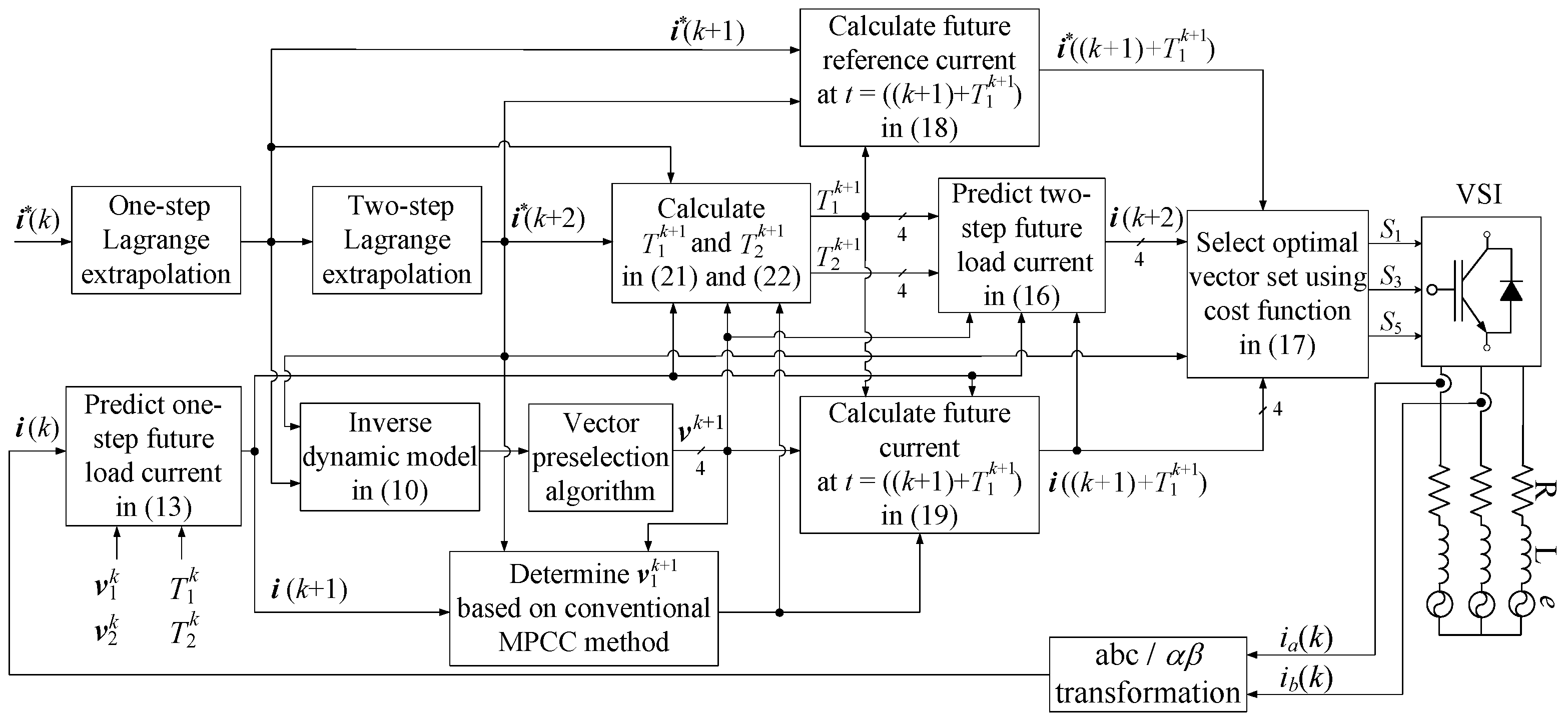
• Measuring the output current $\mathit{i}\left(k\right)$ at the k^th instant.
• Predicting the output current $\mathit{i}\left(k+1\right)$ at the (k + 1)^th instant by using the two voltage vectors ${\mathit{v}}_1^k$ and ${\mathit{v}}_2^k$ during $T_1^k$ and $T_2^k$, respectively, which were determined in the previous (k− 1)^th interval.
• Calculating the reference currents ${\mathit{i}}^{\ast }\left(k+1\right)$ and ${\mathit{i}}^{\ast }\left(k+2\right)$ using (8).
• Obtaining the future voltage vector ${\mathit{v}}^{k+1}$ using the inverse dynamic model (10).
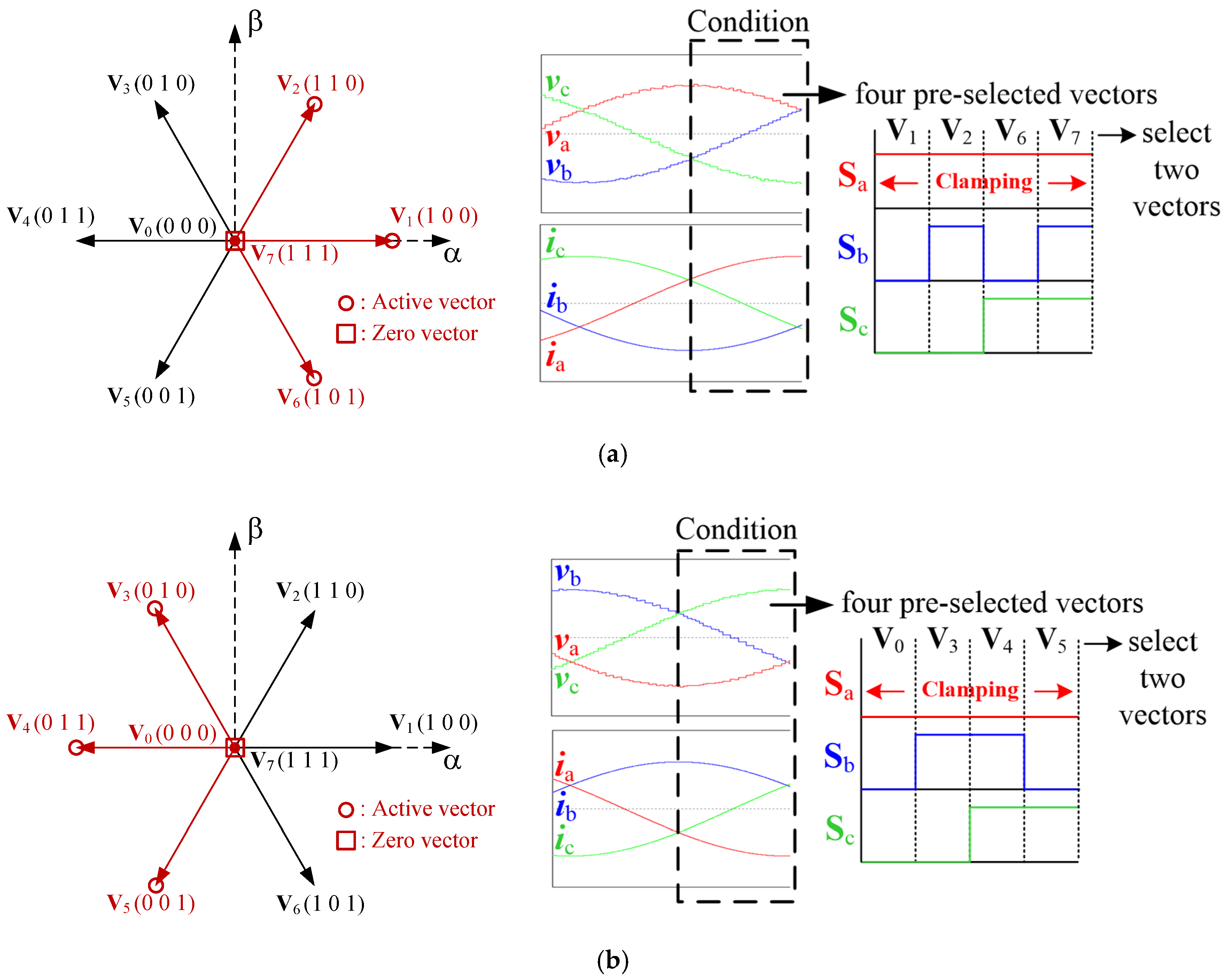
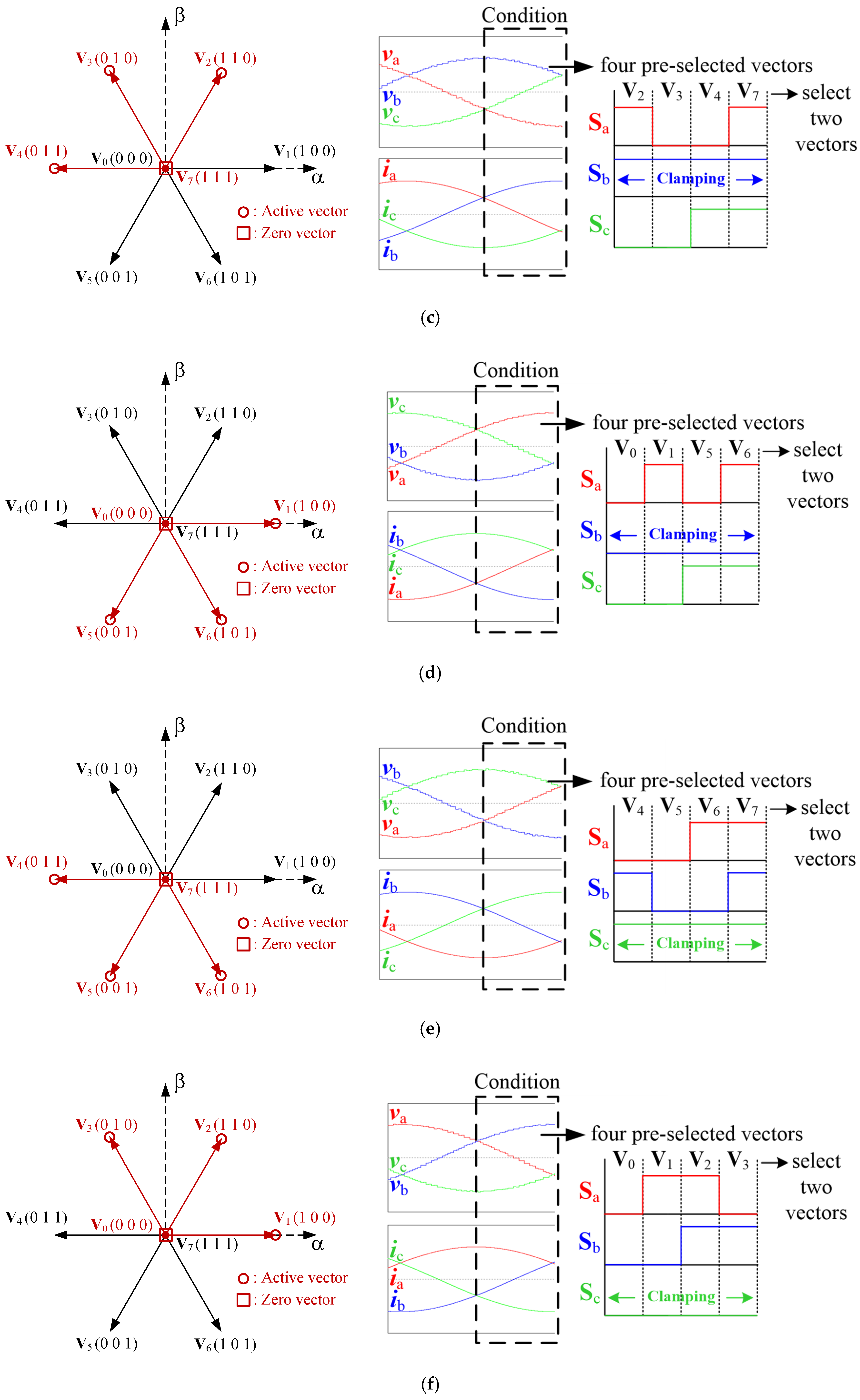
• Sorting the four voltage vectors reducing the switching losses by using the vector pre-selection method.
• Obtaining the initial vector ${\mathit{v}}_1^{k+1}$ by using the conventional MPCC method in the four vectors selected by the vector pre-selection method.
• Calculating the four optimal time durations $T_1^{k+1}$ and $T_2^{k+1}$ according to the initial ${\mathit{v}}_1^{k+1}$ and the second vector ${\mathit{v}}_2^{k+1}$ obtained by using the vector pre-selection method.
• Calculating the output currents $\mathit{i}\left(k+2\right)$ and $\mathit{i}\left(\left(k+1\right)+T_1^{k+1}\right)$ for the pre-selected voltage vectors ${\mathit{v}}_1^{k+1}$ and ${\mathit{v}}_2^{k+1}$ during $T_1^{k+1}$ and $T_2^{k+1}$.
• Calculating the reference currents ${\mathit{i}}^{\ast }\left(\left(k+1\right)+T_1^{k+1}\right)$ using (18).
• Evaluating the four voltage vector sets and corresponding durations by using the G in (17).
• Determining one optimal vector sets with ${\mathit{v}}_1^{k+1}$ and ${\mathit{v}}_2^{k+1}$ along with their optimal durations $T_1^{k+1}$ and $T_2^{k+1}$.
• Storing ${\mathit{v}}_1^{k+1}$, ${\mathit{v}}_2^{k+1}$, $T_1^{k+1}$, and $T_2^{k+1}$ for the next application at the (k + 1)^th instant.

The proposed and conventional methods are compared in terms of current errors, THD values, the total losses, and the number of switchings. The current errors and the THD percentage obtained from the proposed method are shown in Figure 5 a,b, according to the switching frequency because the performance of the VSIs is very much affected by the switching frequency due to its operating principle. The current error between the reference currents and the output currents is decided as

$$error\left(i_x\right)={\displaystyle \sum }_{x=a,b,c}\frac{1}{N}{\displaystyle \sum }_{k=1}^N\left|i_x^{\ast }\left(k\right)-i_x\left(k\right)\right|$$

(23)

where the value of N is set to 10,000, and the error is the average of 10,000 calculated values. As shown in Figure 5a, the proposed method shows the same results in the current error compared to the conventional method.

The THD percentage of the output currents is defined as

$$\%THD=\frac{{{\displaystyle \sum }}_{x=a,b,c}\sqrt{i_{x2}^2+i_{x3}^2+\cdots +i_{xn}^2}}{{{\displaystyle \sum }}_{x=a,b,c}{i}_{x1}}\times 100$$

(24)

where i_x1···i_xn are the fundamental and n^th-harmonic components of the output currents in phase x, respectively. The simulation was set up to the 8335^th-harmonic components. In Figure 5b, the THD of the proposed method is similar to the conventional method.

Power losses of the VSI are calculated to evaluate the switching losses’ reduced performance of the proposed method in the simulation. Power losses can be divided into conduction losses and switching losses. The conduction losses P_cond in an Insulated Gate Bipolar Transistor (IGBT) can be calculated using the following expression:

$$P_{cond}=\left(\frac{1}{T_s}\int V_{CE}\ast I_{C}dt\right)$$

(25)

where $V_{CE}$, $I_C$, and $T_s$ are the collector-emitter voltage, collector current, and sampling period, respectively. In order to determine the constants in (25), a manufacturer’s data sheet is used to apply exponential curve fitting on the on-state loss characteristics [8]. Similarly to the conduction losses, the switching losses P_swit can be calculated using the following expression:

$$P_{swit}=P_{on}+P_{off}=\left(\frac{1}{T_s}\sum E_{on}\right)+\left(\frac{1}{T_s}\sum E_{off}\right)$$

(26)

where $E_{on}$ and $E_{off}$ are turn-on switching loss and turn-off switching loss, respectively. Turn-on switching loss and turn-off switching loss can be obtained by using the loss model with the switching energies obtained from the datasheet of the IGBT module (SKM50GB123D). As shown in Figure 5c, the total losses of the proposed method are lower than those of the conventional method under different switching frequency due to pre-selecting vectors clamping one leg and conducting the largest output current among the three legs.

Figure 5d shows the average number of switchings. In Figure 5d, as the switching frequency increases, the number of switchings of the conventional method and the proposed method increases equally.

4. Results and Comparison

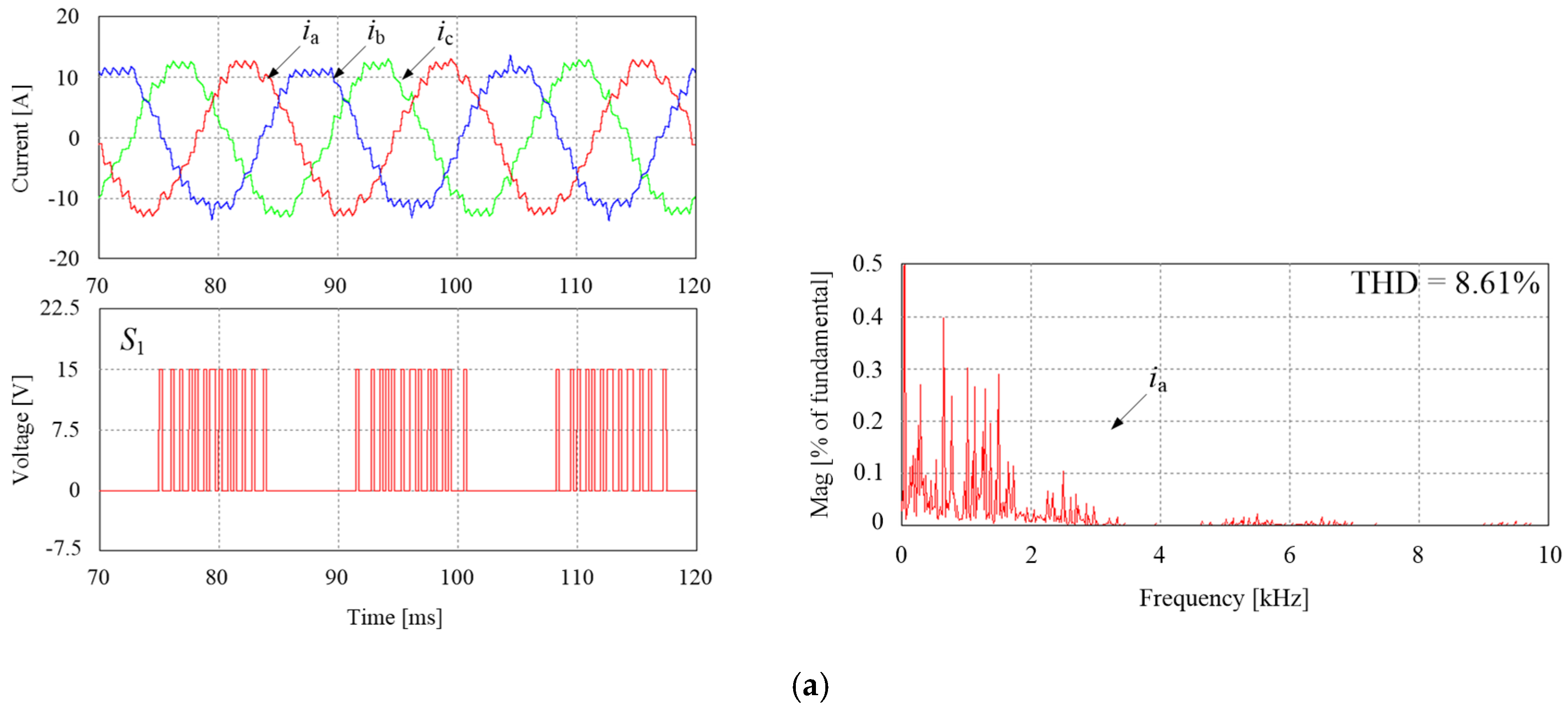
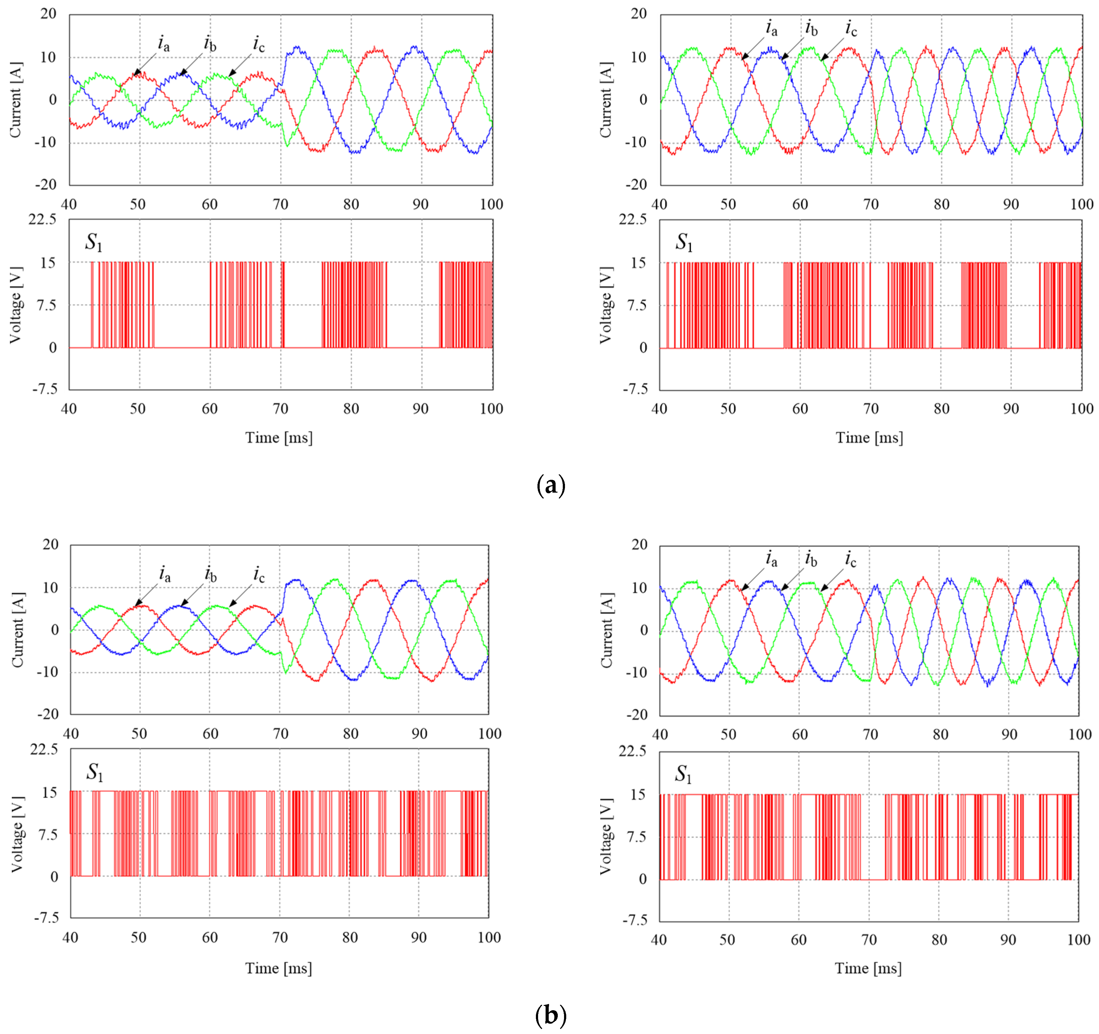
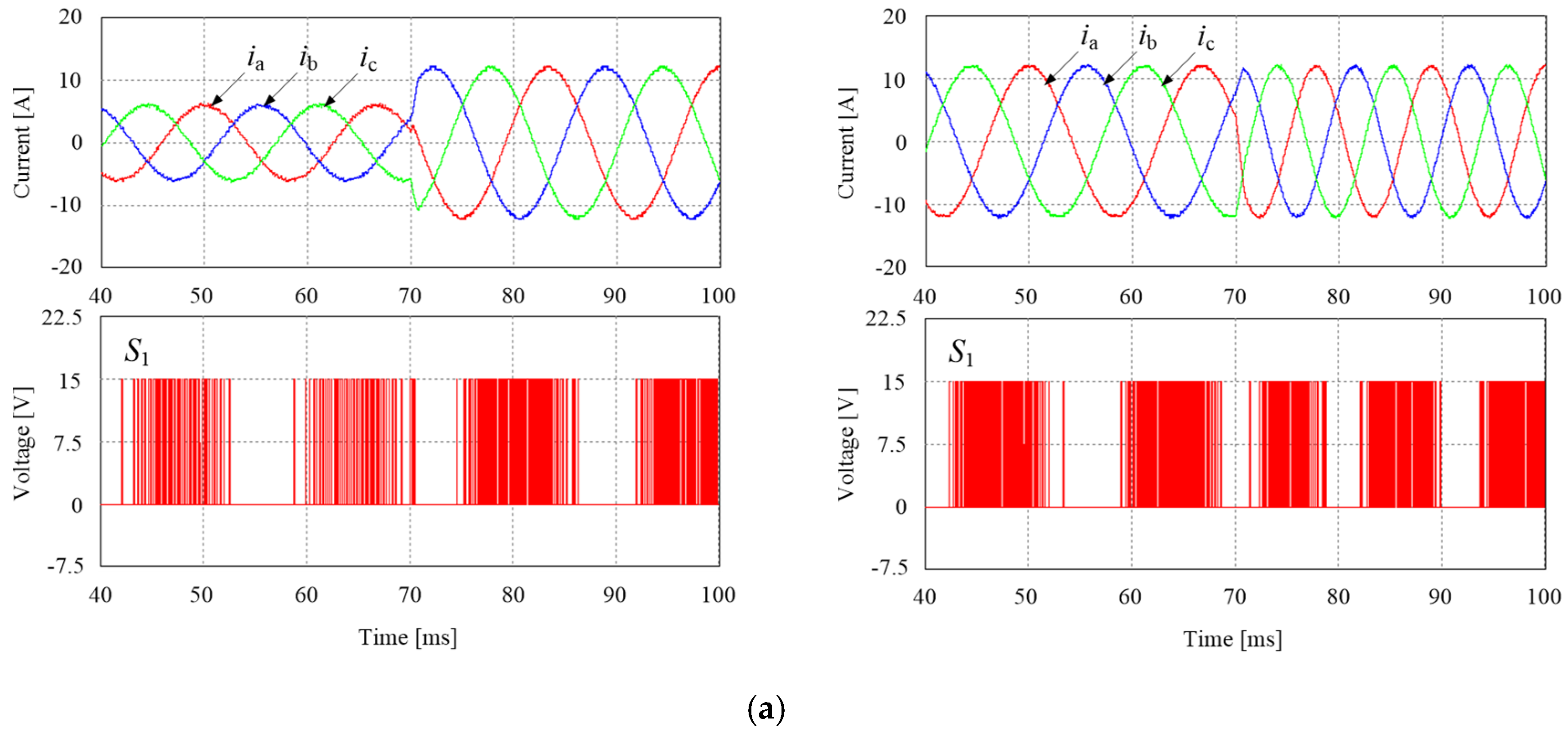
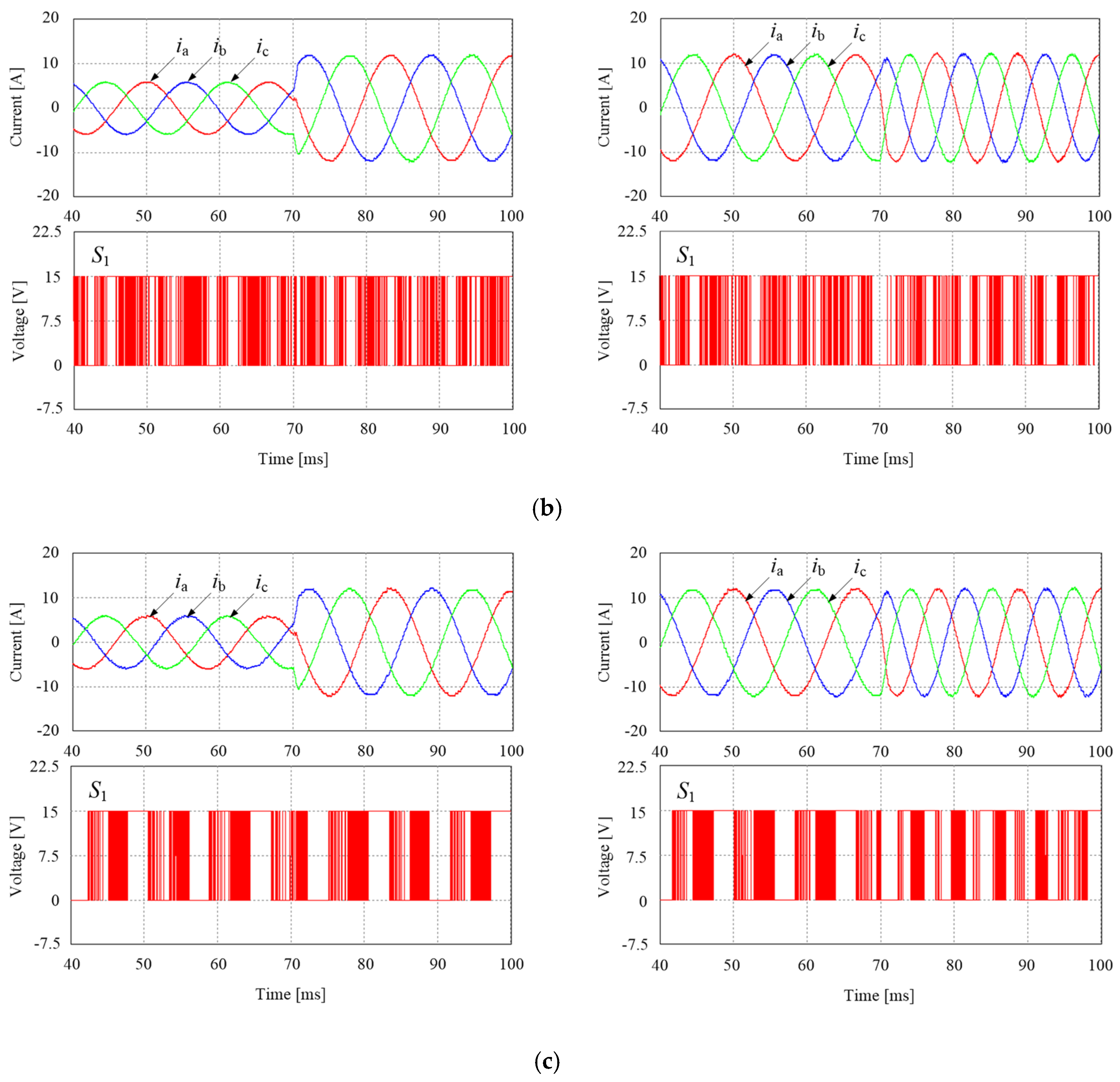
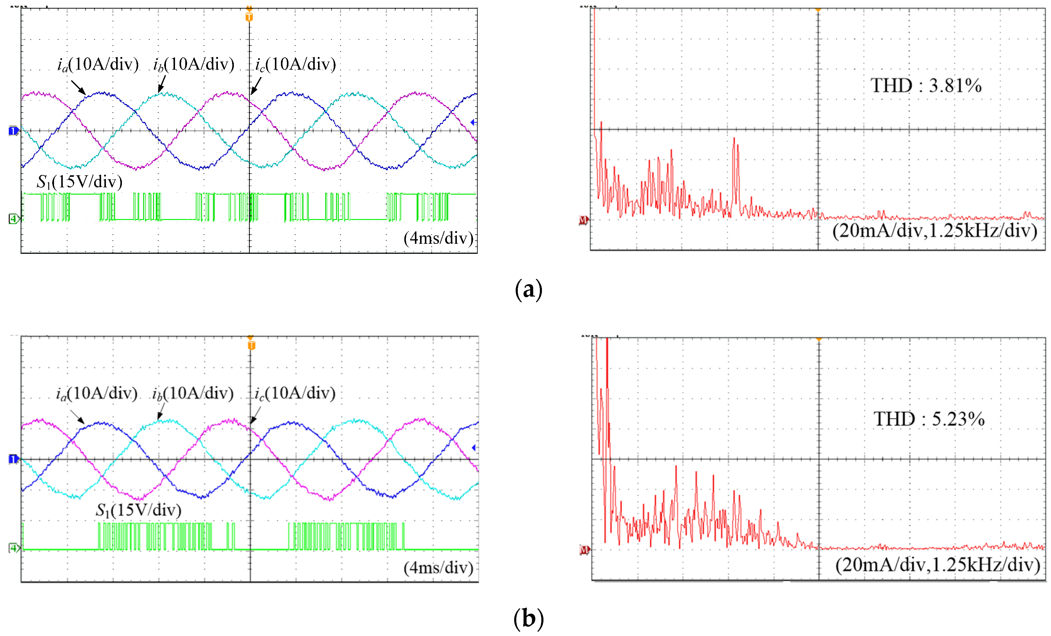
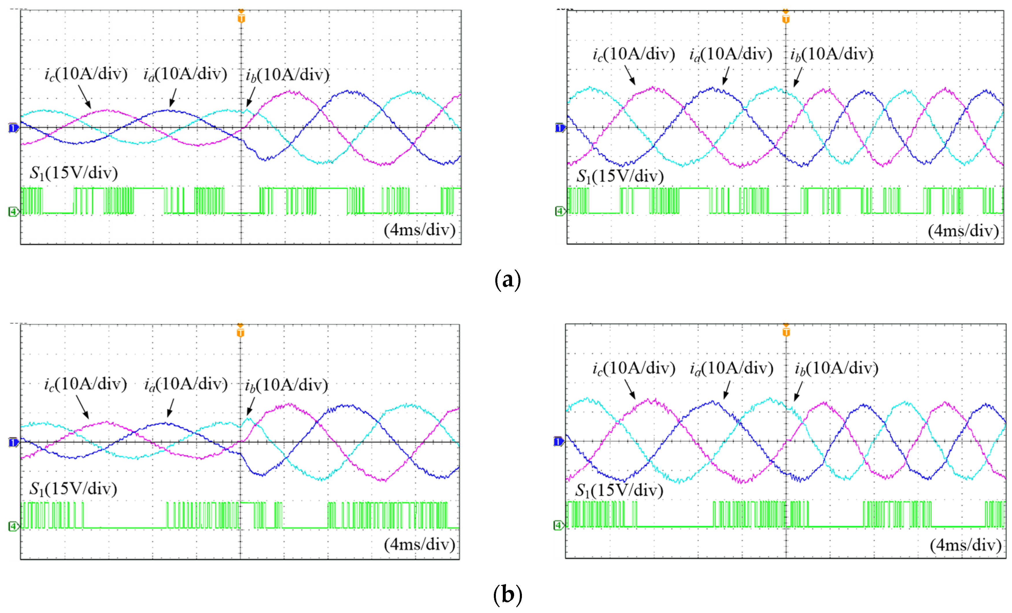
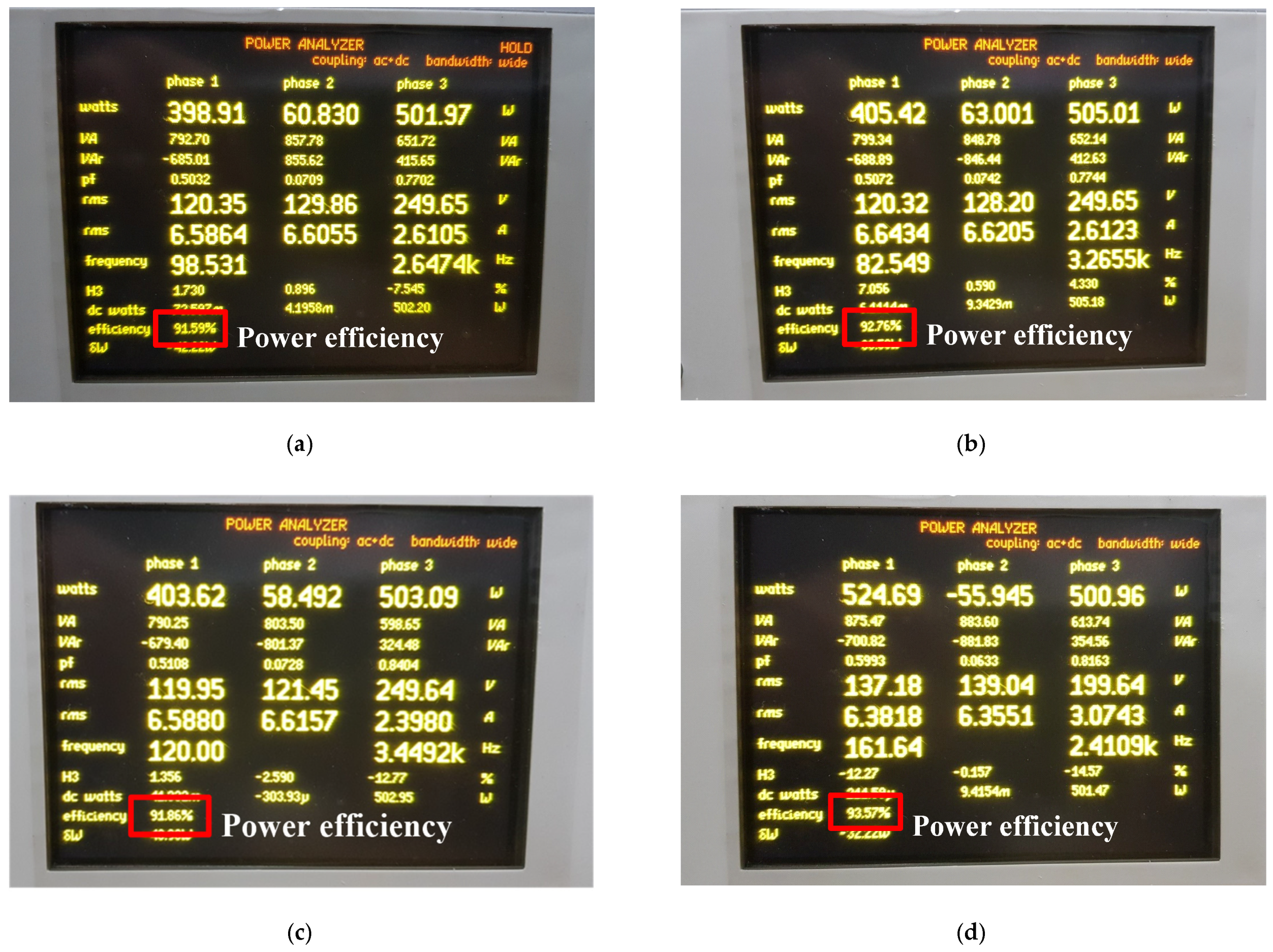
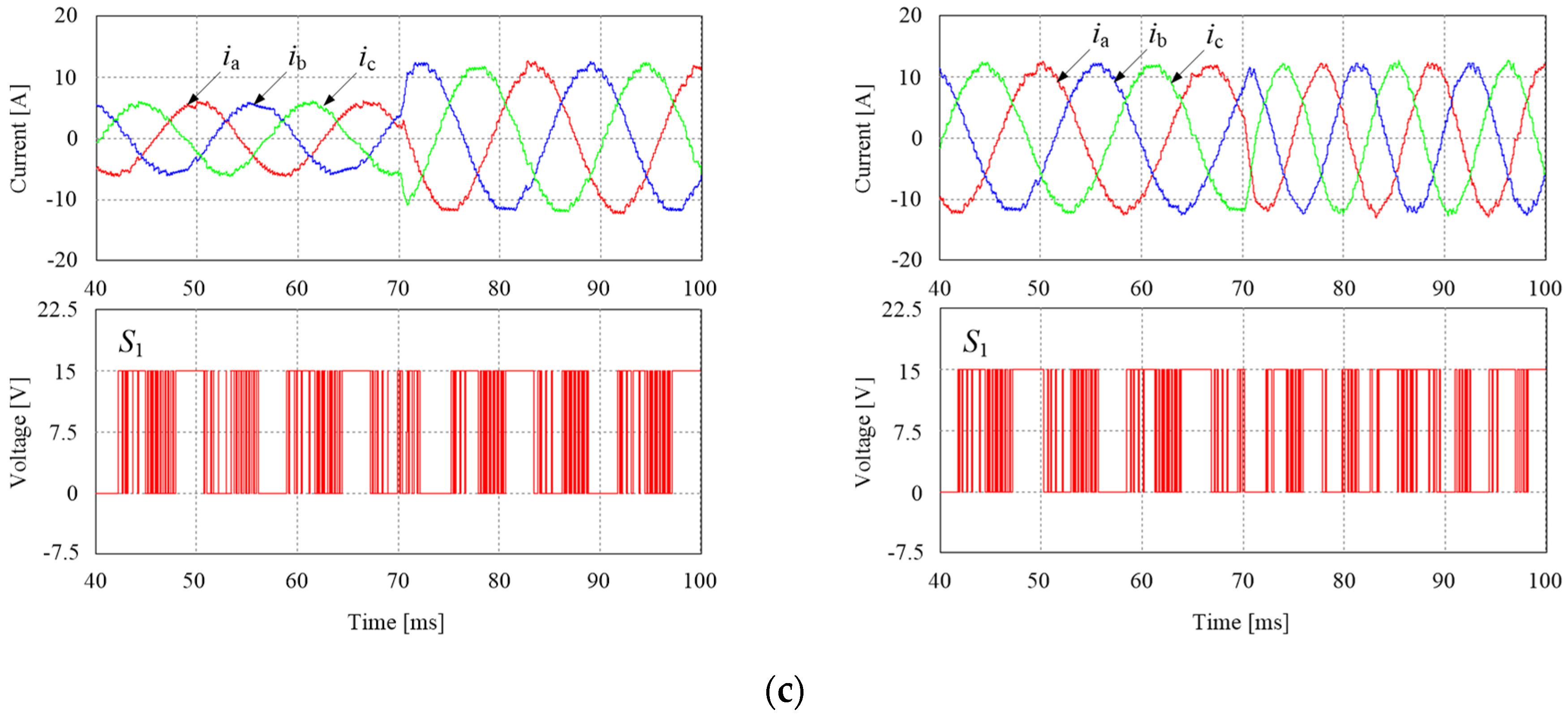
4.1. Simulation and Experimental Results

The simulations were done for the following parameters V_dc = 260 V, the RLe load with R = 0.8 Ω, L = 12 mH, e = 20 V, and the amplitude of the reference current was 12 A. Figure 6 shows the output currents and switching signal S₁ obtained from the conventional method using one vector with T_s = 250 μs, the conventional method using one vector with T_s = 125 μs, the conventional method using two vectors with T_s = 250 μs [19], and the proposed method using two vectors with vector pre-selection method with T_s = 250 μs. Since the proposed method uses two vectors, the sampling period of the conventional method is half of the sampling period of the proposed method in order to compare the two methods. In Figure 6, the output current ripples of the proposed scheme are lower than those of the conventional methods, and the switching signal S₁, which is the upper switch of a-leg, stops operation around the peak output current. Also, the frequency spectrum in Figure 6 shows that the proposed scheme has lower THD values than conventional methods.

Figure 7 shows the output currents and switching signal S₁ obtained from the conventional method using one vector, the conventional method using two vectors [19], and the proposed method when the switching frequency $f_{switching}=4\mathrm{kHz}$ instead of the sampling frequency. As shown in Figure 7, when operating at the same switching frequency, there was no significant difference in high-frequency components between the proposed method and the conventional methods. Also, it can be seen that the clamping was performed well in the proposed method.

The dynamic responses for the conventional method using one vector with T_s = 125 μs, the conventional method using two vectors with T_s = 250 μs, and the proposed method with the T_s = 250 μs are shown in Figure 8. The amplitude of the reference currents was changed from 6 A to 12 A, and the fundamental frequency of the reference currents was changed from 60 Hz to 90 Hz. In both cases, the output currents of the proposed method had a fast dynamic response like those of the conventional methods.

Figure 9 shows the dynamic responses for the conventional method using one vector, the conventional method using two vectors, and the proposed method with switching frequency $f_{switching}=4\mathrm{kHz}$. The amplitude of the reference currents was changed from 6 A to 12 A, and the fundamental frequency of the reference currents was changed from 60 Hz to 90 Hz. In both cases, the output currents of the proposed method had a fast dynamic response like those of the conventional methods.

The MPCC method using two vectors with pre-selection method was implemented by configuring a prototype setup. The experimental setup was composed of the three-phase VSI with the IGBT module and RL load. A digital signal processor (DSP, TMS320F28335) was used to execute the switching algorithm for the VSI. Figure 10 shows the experimental waveforms of the output currents and the switching signal of the switch S₁, which is the upper switch of a-leg. The proposed method was performed under the conditions with T_s = 250 μs, V_dc = 260 V, and the amplitude of the reference current |I^*|= 12 A. In Figure 10, the output current ripples of the proposed method with T_s = 250 μs are less than those of the conventional method with T_s = 125 μs. Besides, the experimental results obtained from the proposed method and the conventional method were comparable to the simulation results, as shown in Figure 6. The switching signal S₁ stopped operation around the peak output current because of the vector pre-selection method. In Figure 10, the THD values were obtained from the digital oscilloscope MSO3054 set up to the 400^th harmonic components, which can be considered to be the maximum number of harmonics.

The dynamic responses of the proposed method with the sampling period T_s = 250 μs and the conventional method with T_s = 250 μs are shown in Figure 11. The amplitude of the reference currents was changed from 6 A to 12 A, and the fundamental frequency of the reference currents was changed from 60 Hz to 90 Hz. In the step changes of magnitude and fundamental frequency of the reference currents, the output currents of the proposed method tracked the reference change as fast as those of the conventional method with half the sampling period.

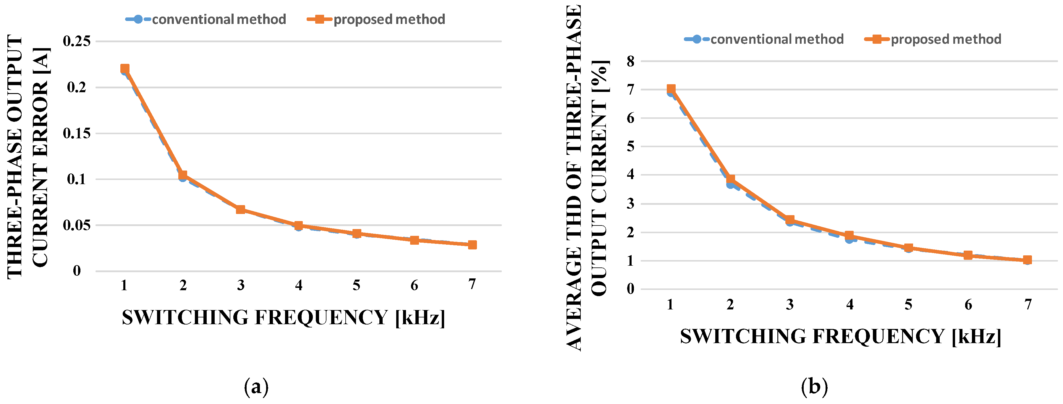
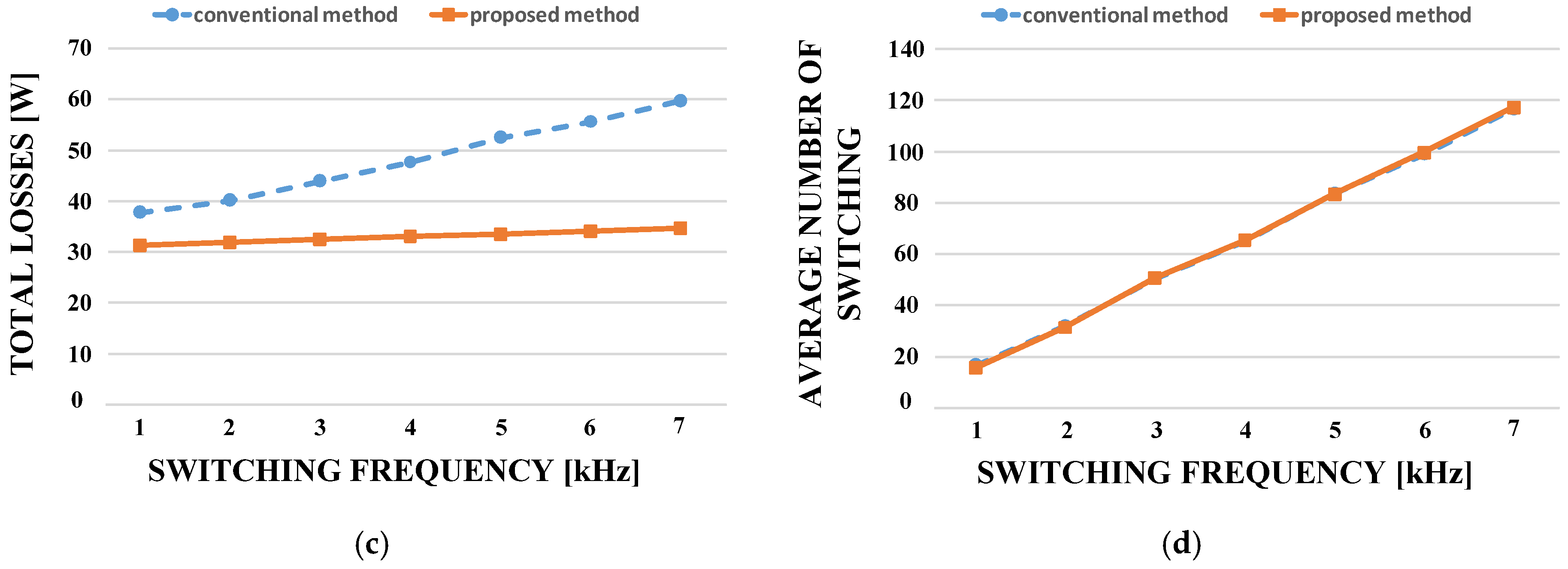
4.2. Performance Comparison

In order to evaluate the superiority of the proposed method in terms of efficiency, experimental data of loss and power efficiency were measured in the conventional and the proposed methods. The losses were measured with a power meter (Precision Power Analyzer 5500—Newtons 4th) in the experimental setup. The three conventional MPCC methods were compared:

(1)

Conv. (1 vector): MPCC method using a single optimal voltage vector [3] with the same sampling period with the proposed method.

(2)

Conv. (1 vector): MPCC method using a single optimal voltage vector [3] with half sampling period of the proposed method

(3)

Conv. (2 vectors): MPCC method using two optimal voltage vectors [19].

Figure 12 shows the power efficiency of the conventional methods and the proposed method measured by PPA. As shown in Figure 11, the power efficiency of the conventional method using one vector with T_s = 125 μs showed the worst efficiency, and it is because the sampling frequency is twice as large as the other methods. When the sampling period was equal to 250 μs, the conventional method using two vectors showed the worst efficiency because this method uses two vectors during one sampling period. It can be clearly seen that the proposed method resulted in the highest efficiency because the clamping operation of switches exposed to highest current conduction can reduce the switching losses.

Table 2. Performance comparison of the conventional methods and the proposed method.

	THD [%]	Current Error [A]	Execution Time [μs]	Losses [W]	Power Efficiency [%]	${\mathit{T}}_{\mathit{s}}\left[\mathsf{\mu }\mathbf{s}\right]$	${\mathit{f}}_{\mathit{s}}\left[\mathbf{kHz}\right]$
Conv (1 vector)	4.48	0.083	5.15	42.23	91.59	125	8
	8.61	0.158	5.15	36.59	92.76	250	4
Conv (2 vectors)	3.96	0.111	19.04	40.98	91.86	250	4
Proposed	3.87	0.105	22.06	32.215	93.57	250	4

shows the performance comparison of the conventional methods and the proposed method. The conventional method using one vector during one sampling period showed high THD values of the output currents. To overcome this drawback, control methods using two vectors during one sampling period have been studied [19]. Although this method can improve the current quality by decreasing THD values of the output currents, it increases switching losses because of the usage of two vectors during one sampling period. The proposed method not only improved the THD values of the output currents by using two optimal vectors during one sampling period but also reduced the switching loss by clamping switches exposed to highest current conduction. On the other hand, the execution time in the digital signal processor of the proposed method could be higher than the conventional methods because of the complexity of the proposed method, which needs the technique to pre-select the vectors and choose two vectors.

In addition,

Table 3. Performance comparison between the conventional method and the proposed method in simulation results.

	THD [%]	Losses [W]	Power Efficiency [%]	${\mathit{T}}_{\mathit{s}}\left[\mathsf{\mu }\mathbf{s}\right]$	${\mathit{f}}_{\mathit{s}}\left[\mathbf{kHz}\right]$
Conv (1 vector)	4.48	40.28	91.94	125	8
Proposed	3.87	31.12	93.78	250	4

and

Table 4. Performance comparison between the conventional method and the proposed method in experimental results.

	THD [%]	Losses [W]	Power Efficiency [%]	${\mathit{T}}_{\mathit{s}}\left[\mathsf{\mu }\mathbf{s}\right]$	${\mathit{f}}_{\mathit{s}}\left[\mathbf{kHz}\right]$
Conv (1 vector)	5.23	42.23	91.59	125	8
Proposed	3.81	32.215	93.57	250	4

show performance comparisons between the conventional method and the proposed method in the simulation and experimental results, respectively. As shown in Table 3 and Table 4, the THD values and the total losses of the proposed method were lower than those of the conventional method, with the half sampling frequency of the proposed method.

Table 5. Performances of the proposed method obtained in simulation and experimental results.

	THD [%]	Losses [W]	Power Efficiency [%]
Simulation	3.87	31.12	93.78
Experiment	3.81	32.215	93.57

depicts the results of the proposed method obtained in simulation and experimental result, where data were almost similar.

5. Conclusions

In this paper, the MPCC method for three-phase VSI based on the utilization of two vectors has been proposed to regulate output currents with small current errors and current ripples. Also, the vector pre-selection method is applied to the proposed method to reduce the VSIs switching losses by pre-selecting the four available voltage vectors. In the proposed method, selecting two future voltage vectors among the four available voltage vectors and dividing them in a future sampling period are determined by the newly defined cost function and the optimization process. The proposed method reduces the total loss versus the conventional MPCC method with the same switching frequency due to the optimal process involved in selecting two vectors and their time durations. In addition, the proposed method and the conventional method show the same performance in current error and THD. The effectiveness of the proposed method is verified from the study of the simulation and experiment of the three-phase VSIs.

References

- Liang, D.; Li, J.; Qu, R.; Kong, W. Adaptive second-order sliding-mode observer for PMSM sensorless control considering VSI nonlinearity. IEEE Trans. Power Electron. 2018, 33, 8994–9004. [Google Scholar] [CrossRef]
- Kinnares, V.; Charumit, C. Modulating functions of space vector PWM for three-leg VSI-fed unbalanced two-phase induction motors. IEEE Trans. Power Electron. 2009, 24, 1135–1139. [Google Scholar] [CrossRef]
- Kouro, S.; Cortes, P.; Vargas, R.; Ammann, U.; Rodriguez, J. Model predictive control—A simple and powerful method to control power converters. IEEE Trans. Ind. Electron. 2009, 56, 1826–1838. [Google Scholar] [CrossRef]
- Cortes, P.; Rodriguez, J.; Silva, C.; Flores, A. Delay compensation in model predictive current control of a three-phase inverter. IEEE Trans. Ind. Electron. 2012, 59, 1323–1325. [Google Scholar] [CrossRef]
- Kwak, S.; Park, J.C. Switching strategy based on model predictive control of VSI to obtain high efficiency and balanced loss distribution. IEEE Trans. Power Electron. 2014, 29, 4551–4567. [Google Scholar] [CrossRef]
- Cortes, P.; Rodriguez, J.; Antoniewicz, P.; Kazmierkowski, M. Direct power control of an AFE using predictive control. IEEE Trans. Power Electron. 2008, 23, 2516–2523. [Google Scholar] [CrossRef]
- Jun, E.-S.; Kwak, S. Performance comparison of model predictive control methods for active front end rectifiers. IEEE Access 2018, 6, 77272–77288. [Google Scholar] [CrossRef]
- Gong, Z.; Wu, X.; Dai, P.; Zhu, R. Modulated model predictive control for MMC-based active front-end rectifiers under unbalanced grid conditions. IEEE Trans. Ind. Electron. 2019, 66, 2398–2409. [Google Scholar] [CrossRef]
- Vargas, R.; Cortes, P.; Ammann, U.; Rodriguez, J.; Pontt, J. Predictive control of a three-phase neutral-point-clamped inverter. IEEE Trans. Ind. Electron. 2007, 54, 2697–2705. [Google Scholar] [CrossRef]
- Yaramasu, V.; Wu, B.; Rivera, M.; Narimani, M.; Kouro, S.; Rodriguez, J. Generalised approach for predictive control with common-mode voltage mitigation in multilevel diode-clamped converters. IET Power Electron. 2015, 8, 1440–1450. [Google Scholar] [CrossRef]
- Townsend, C.D.; Summers, T.J.; Vodden, J.; Watson, A.J.; Betz, R.E.; Clare, J.C. Optimization of switching losses and capacitor voltage ripple using model predictive control of a cascaded H-bridge multilevel statcom. IEEE Trans. Power Electron. 2013, 28, 3077–3087. [Google Scholar] [CrossRef]
- Jun, E.-S.; Kwak, S. A Highly Efficient Single-Phase Three-Level Neutral Point Clamped (NPC) Converter Based on Predictive Control with Reduced Number of Commutations. Energies 2018, 11, 3524. [Google Scholar] [CrossRef]
- Rivera, M.; Rojas, C.; Rodriguez, J.; Espinoza, J. Methods of source current reference generation for predictive control in a direct matrix converter. IET Power Electron. 2013, 6, 894–901. [Google Scholar] [CrossRef]
- Siami, M.; Khaburi, D.R.; Rodriguez, J. Simplified finite control set-model predictive control for matrix converter-fed PMSM drives. IEEE Trans. Power Electron. 2018, 33, 2438–2446. [Google Scholar] [CrossRef]
- Wang, L.; Dan, H.; Zhao, Y.; Zhu, Q.; Peng, T.; Sun, Y.; Wheeler, P. A Finite control set model predictive control method for matrix converter with zero common-mode voltage. IEEE J. Emerg. Sel. Top. Power Electron. 2018, 6, 327–338. [Google Scholar] [CrossRef]
- Kwak, S.; Moon, S. Model Predictive Control Methods to Reduce Common-Mode Voltage for Three-Phase Voltage Source Inverters. IEEE Trans. Power Electron. 2015, 30, 5019–5035. [Google Scholar] [CrossRef]
- Blaabjerg, F.; Jaeger, U.; Nielsen, S.M.; Pedersen, J.K. Power losses in PWM-VSI inverter using NPT or PT IGBT devices. IEEE Trans. Power Electron. 1995, 10, 358–367. [Google Scholar] [CrossRef]
- Zhang, Y.; Yang, H. Model predictive torque control of induction motor drives with optimal duty cycle control. IEEE Trans. Power Electron. 2014, 29, 6593–6603. [Google Scholar] [CrossRef]
- Park, S.Y.; Kwak, S. Comparative study of three model predictive current control methods with two vectors for three-phase DC/AC VSIs. IET Electron. Power Appl. 2017, 11, 1284–1297. [Google Scholar] [CrossRef]
- Nguyen, H.T.; Jung, J.-W. Asymptotic stability constraints for direct horizon-one model predictive control of SPMSM drives. IEEE Trans. Power Electron. 2018, 33, 8213–8219. [Google Scholar] [CrossRef]
- Mwasilu, F.; Kim, E.-K.; Fafaq, M.S.; Jung, J.-W. Finite-set model predictive control scheme with an optimal switching voltage vector technique for high-performance IPMSM drive applications. IEEE Trans. Ind. Inform. 2018, 14, 3840–3848. [Google Scholar] [CrossRef]
- Zhang, Y.; Yang, H.; Xia, B. Model predictive torque control of induction motor drives with reduced torque ripple. IET Elect. Power Appl. 2015, 9, 595–604. [Google Scholar] [CrossRef]
- Kwak, S.; Park, J.-C. Model-predictive direct power control with vector preselectiontechnique for highly efficient active rectifiers. IEEE Trans. Ind. Inform. 2015, 11, 44–52. [Google Scholar] [CrossRef]
- Zhang, Y.; Peng, Y.; Yang, H. Performance improvement of two-vectors-based model predictive control of PWM rectifier. IEEE Trans. Power Electron. 2016, 31, 6016–6030. [Google Scholar] [CrossRef]
- Zhang, Y.; Yang, H. Two-vector-based model predictive torque control without weighting factors for induction motor drives. IEEE Trans. Power Electron. 2016, 31, 1381–1390. [Google Scholar] [CrossRef]
- Kwak, S.; Park, J.-C. Predictive control method with future zero-sequence voltage to reduce switching losses in three-phase voltage source inverters. IEEE Trans. Power Electron. 2015, 30, 1558–1566. [Google Scholar] [CrossRef]