Article

Accurate Rigid Body Localization Using DoA Measurements from a Single Base Station

1
School of IoT Engineering, Jiangnan University, Wuxi 214122, China
2
Jiangsu Key Construction Laboratory of IoT Application Technology, Wuxi 214122, China
3
Department of Electrical and Computer Engineering, University of Canterbury, Christchurch 8020, New Zealand
4
Department of Electronic Engineering, Kwangwoon University, Seoul 139-701, South Korea
*
Author to whom correspondence should be addressed.
Electronics 2019, 8(6), 622; https://doi.org/10.3390/electronics8060622
Submission received: 3 May 2019 / Revised: 26 May 2019 / Accepted: 29 May 2019 / Published: 1 June 2019
(This article belongs to the Section Microwave and Wireless Communications)

Abstract

:
Rigid body localization (RBL) is to simultaneously estimate the position and attitude of a rigid target. In this paper, we focus on the RBL problem using a single base station (BS) and direction of arrival (DoA) measurements. Several wireless sensors are mounted on the rigid body of interest, and their topology information is known a priori. The single BS measures the DoAs of wireless sensor signals and fuses them with the sensor topology information to estimate the position and orientation of the rigid body and achieve RBL. We propose two RBL methods, namely, the observation matching (OM) algorithm and topology matching (TM) algorithm with refinement. The emerging participatory searching algorithm (PSA) is adopted in both methods to solve the nonlinear matching problems. Simulations show that, compared with the existing approach, the OM method can achieve better RBL accuracy under high DoA noise levels, while the performance of the TM algorithm with refinement is closer to the constrained Cramér–Rao bound (CCRB) under low DoA noise levels.

1. Introduction

1.1. Background

A rigid body is a solid body whose deformation can be neglected. Large rigid bodies include airplanes, ships, and vehicles, while virtual reality (VR) helmets, human bodies, and heads of robots are typical small rigid bodies. Rigid body localization (RBL) estimates, relative to a predetermined reference frame, both the position and attitude of a rigid object in three-dimensional (3-D) space [1,2].
High-precision position and attitude information of a rigid object are essential for many military and civilian applications. For example, RBL can be used to acquire the 3-D position and orientation of unmanned aerial vehicles (UAVs) [3], aircrafts, and submarines. It can also be applied to monitor the tilts of buildings and bridges in real time. In VR systems, both the position and attitude information of the VR helmet are necessary for providing a corresponding virtual picture [4]. Last but not least, in the intelligent parking scenario, the position and heading direction of the vehicle are indispensable [5].

1.2. Related Works

Conventionally, the position and attitude estimation for an object have been investigated separately. Among the positioning technologies, the Global Navigation Satellite System (GNSS) is well-known but only efficient in open outdoor environments. Alternatively, in wireless sensor networks (WSNs), the location of the object can be found by observing the signal from wireless devices equipped on the target [6,7,8]. For fine-grained positioning, commonly used parameters are the time of arrival (ToA), time difference of arrival (TDoA), and direction of arrival (DoA), to just list a few.
As for the attitude estimation for rigid objects, the use of an inertial measurement unit (IMU), such as the gyro sensor [9] or the three-axis magnetometer [10], is a straightforward choice. However, IMU-based attitude estimation suffers from long-term unilateral error accumulation, while the three-axis magnetometer is based on the strength of Earth’s magnetic field, which may be affected by complex ground environments. In addition, these attitude estimation schemes alone are not able to provide the position information of a rigid object at the same time.
For simultaneously determining the position and attitude of a rigid target, several techniques have been proposed in literature. An efficient approach for the RBL of outdoor, large-scale rigid bodies was developed based on the GNSS [11,12,13]. In this scheme, the absolute position was determined by pseudo-range observations, while the attitude was estimated from the measured carrier phases of the satellite signals received at multiple GNSS antennas. However, application of the above GNSS-based scheme was restricted to outdoor scenarios, and the use of multiple GNSS antennas led to higher implementation costs. Computer vision-based RBL is another popular solution [14,15]. This scheme uses a single (or multiple) theodolite to find the 3-D coordinates of feature points on the rigid body, and then it applies methods like singular value decomposition (SVD) [16] to obtain the relative displacement vector and attitude information with respect to the reference frame. Although this method has high estimation accuracy, its performance relies heavily on the precise coordinate observations of feature points, which poses significant demand for light conditions as well as on computational resources.
The RBL approaches based on small-scale WSNs can mitigate the weakness of the aforementioned two RBL schemes. In general, the WSN-based technique is implemented as follows. Firstly, several wireless sensors are mounted on the surface of the rigid body, which transforms the point target into an extended one. Next, the physical observations of wireless sensor signals are acquired by the base stations (BSs) (i.e., the anchor nodes). Finally, the 3-D position and attitude information of the rigid object are obtained by fusing the known topology information of the wireless sensors and sensor signal observations.
State-of-the-art WSN-based RBL schemes mainly consider the use of ToA measurements (also referred to as the range measurements) to determine sensor-BS distances, which are then exploited with the topology information for RBL [17,18,19,20]. In the ToA-based RBL model, the position and attitude of the rigid body relative to a reference frame are obtained via finding the associated rotation matrix and translation vector. This is a challenging problem, because the rotation matrix to be determined belongs to the 3-D special orthogonal S O ( 3 ) group. In [18], the authors first linearized the RBL model by adopting a squared-range (SR) formulation. They then proposed to use a serial of unitarily constrained least square estimators to compute the estimate of the target position and orientation. The Cramér–Rao lower bound (CRLB) for the ToA-based RBL task was also derived. To further improve computation efficiency, authors in [19] employed the divide and conquer (DAC) strategy and developed a noniterative algorithm with higher RBL accuracy obtained via a refinement stage. Alternatively, a semidefinite relaxation (SDR) technique was adopted to find the maximum likelihood (ML) solution to ToA-based RBL [20,21]. The developed SDR-based methods were shown to have better performances under high noise levels.
Nevertheless, deficiencies of the ToA-based RBL solutions are also obvious. First, it requires three or more BSs spatially separated at known, fixed positions. This will increase system complexity, and it may even be impractical in circumstances such as spacecraft docking or where the BSs are moving. Another aspect is that it has high requirement for time synchronization between wireless sensors and BSs, which is quite challenging in practice.
The DoAs of the wireless signal can be obtained via applying array signal processing techniques [22], and they can be used for RBL as well. As an alternative to ToA, the DoA measurement completely eliminates the need for precise sensor BS synchronization. In addition, two-dimensional (2-D) DoA information, namely the azimuth and pitch angles, makes it possible to perform RBL using a single BS [23]. Last, DoA estimation methods are readily available. For example, the estimation of signal parameters via rotational invariance technique (ESPRIT) and multiple signal classification (MUSIC) algorithms are widely adopted DoA estimators. In this paper, we shall consider RBL based on the DoAs obtained at a single BS.

1.3. Contributions

Similar to existing ToA-based schemes, we assume in this paper that several wireless sensors have already been mounted on the rigid body of interest, and their topology is known precisely. DoA information of these wireless sensors is measured by the BS. By fusing the DoA measurements with the wireless sensor topology, the RBL is achieved. In this paper, we present two methods for the RBL task, namely the observation matching (OM) algorithm and the enhanced topology matching (TM) algorithm with refinement. Both methods utilize an emerging population-based optimization framework called participatory searching algorithm (PSA) [24]. Our contributions are summarized as follows.
(1) In the OM method, we first exploit the multidimensional scaling (MDS) technique [25] to fuse the wireless sensor topology information and obtain the reference frame. Then, the reference frame undergoes an instantaneously determined translation and rotation, and the current frame is obtained. The theoretical 2-D DoA of each sensor in the obtained current frame is then compared against the actual DoA measurements to search for the optimal translation and rotation parameters. In this way, the unknown translation and rotation parameters applied to the reference frame can be found, which accomplishes the RBL task.
(2) The TM method with refinement has three processing steps. In Step 1, the 3-D coordinates of all wireless sensors are expressed in terms of the DoA measurements by iteratively matching the estimated sensor topology against the known topology information. We obtain the sensor coordinates as the coarsely estimated current frame. In Step 2, we conduct a refinement process using the weighted least squares (WLS) technique to better explore the noise-free sensor topology information and update the coarsely estimated sensor coordinates in Step 1. In Step 3, the translation vector and rotation matrix that relate the refined current frame to the reference frame are found via an SVD-based approach.
(3) As a benchmark for evaluating the performance of the two proposed methods, we present in detail the derivation of the constrained Cramér–Rao bound (CCRB) for the considered problem of RBL using DoAs from a single BS. The constraint is from the fact that the rotation matrix to be estimated belongs to the S O ( 3 ) group.
The rest of the paper is organized as follows. In Section 2, we formulate the single BS RBL problem in consideration and derive the CCRB. The two proposed RBL approaches are presented in Section 3. A brief introduction and the realization of the PSA algorithm are given in Section 4. In Section 5, through simulations, we evaluate the performance of proposed RBL approaches. Finally, the conclusion is drawn in Section 6.
For clarity, we denote matrices and vectors with upper-case and lower-case bold-face letters. tan 1 ( ) represents 1/ tan ( ) . X T is the transpose of X , and x ^ denotes the estimate of x . | | | | represents the Euclidian norm, and is the Kronecker product. I n is the n -by- n identity matrix. vec ( X ) and Rank ( X ) are, respectively, a column vector obtained by stacking the columns of the matrix X and the rank of X . diag ( x ) is a diagonal matrix with its diagonal elements equal to the elements in x .

2. Problem Formulation and Constrained Cramér–Rao Bound (CCRB)

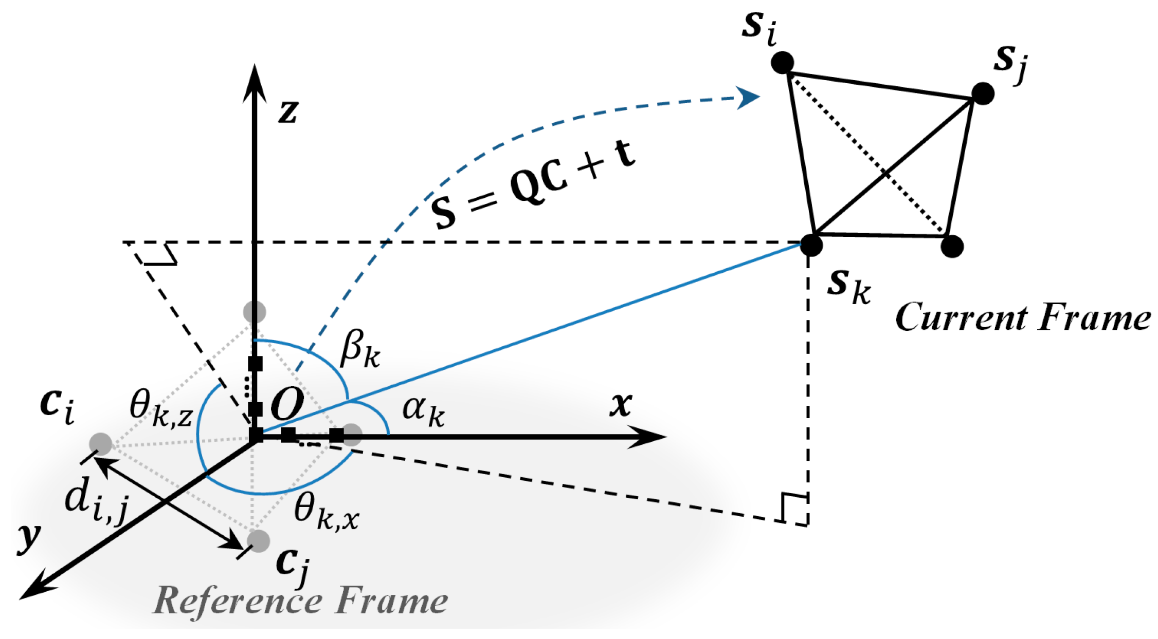
2.1. Rigid Body Localization (RBL) Based on Direction of Arrival (DoA) Measurements from a Single Base Station (BS)

To decide the position and orientation of a rigid body in 3-D space, we mounted K wireless sensors on the rigid object surface to serve as feature points. In the reference frame, the position of the k -th sensor was denoted as c k = [ c x , k , c y , k , c z , k ] T . Collecting them yielded C = [ c 1 , , c K ] 3 × K . The sensor positions c k under the reference frame can be determined by the known sensor topology information. They are known quantities, as will be evident in the next section. Without the loss of generality, the reference frame was set to be at the origin O where the single BS was located.
On the other hand, under the current frame of the rigid body, which is to be estimated, the 3-D coordinates of wireless sensors were collected in S = [ s 1 , , s K ] 3 × K . Here, s k = [ s x , k , s y , k , s z , k ] T are the 3-D coordinates of the k -th sensor under the current frame. According to the rigid body transformation rule [16], S can be obtained by applying to C a rotation and translation (see Figure 1). Mathematically, we have:
S = Q C + t 1 1 × K ,
where t = [ x , y , z ] T is the unknown translation vector. Q is the unknown rotation matrix and it belongs to the 3-D orthogonal group:
S O ( 3 ) = { Q 3 × 3 : Q Q T = Q T Q = I 3 , det ( Q ) = 1 } .
Q can also be specified using the Euler angles (i.e., roll ϕ (rotation about x -axis), pitch φ (rotation about y -axis), and yaw ψ (rotation about z -axis)). Mathematically, Q can be expressed as [25]:
Q = [ q 1 , q 2 , q 3 ] T = [ c φ c ψ c φ s ψ s φ s ϕ s φ c ψ c ϕ s ψ s ϕ s φ s ψ + c ϕ c ψ s ϕ c φ c ϕ s φ c ψ + s ϕ s ψ c ϕ s φ s ψ s ϕ s ψ s ϕ c φ ] ,
where s x and c x represent sin x and cos x , respectively.
The RBL of a rigid body requires estimating the translation vector t and rotation matrix Q . For this purpose, two pieces of information are utilized in this work. The first one is the exactly known topology information of the wireless sensors. If the full-connected scenario is considered, the sensor topology information is embedded in K ( K 1 ) 2 Euclidean distances among all sensor pairs [26]. They can be collected in a column vector:
d = [ d 1 , 2 , , d i , j , , d K 1 , K ] T , i , j = 1 , , K , j > i ,
where d i , j = | | c i c j | | = | | s i s j | | is the Euclidean distance between i -th and j -th sensors.
Another piece of information for RBL is provided by the BS at the origin. They are the 2-D DoAs of the wireless sensor signals. We assumed that the BS was equipped with an L-shaped antenna array (LSAA). In particular, sufficient antenna elements were deployed along the x - and z -axes to measure the angles between the arriving signal directions of the K sensors and the x - and z -axes, which were denoted as α = [ α 1 , , α K ] and β = [ β 1 , , β K ] , respectively, as shown in Figure 1. Discussions on specific DoA estimation techniques are beyond the scope of this paper and interested readers are directed to, e.g., [27]. We assume the measured DoAs of the k -th sensor, α k and β k , are subject to independent Gaussian noise such that:
d = [ d 1 , 2 , , d i , j , , d K 1 , K ] T , i , j = 1 , , K , j > i ,
where [ α k o , β k o ] T collects the true DoA values.
We are interested in determining the translation vector t and rotation matrix Q that relate the reference frame to the current frame (see (1)) from the noise-free sensor distance information in d (see (4)) and 2-D DoA measurements in (5).

2.2. CCRB

We shall derive the CCRB for the DoA-based RBL problem formulated in the previous section. The parameters to be estimated included the translation vector t = [ x , y , z ] T and the rotation matrix Q . We introduced a 12 × 1 composite unknown vector ρ = [ q 1 T , q 2 T , q 3 T , t T ] T . Because Q belonged to S O ( 3 ) (see (2)), the unknown vector ρ was then subject to equality constraints. The associated CCRB of ρ has form [28]:
C C R B ( ρ ) U ( U T F ( ρ ) U ) 1 U T ,
where U 12 × P depends on the equality constraints from (2), and P is the number of the constraints. F ( ρ ) 12 × 12 is the unconstrained Fisher information matrix (FIM) of the composite unknown vector ρ . We shall provide their definitions below.
According to (2), ρ satisfies the following P = 6 equality constraints:
h ( ρ ) = [ q 1 T q 1 1 , q 2 T q 2 1 , q 3 T q 3 1 , q 1 T q 2 , q 1 T q 3 , q 2 T q 3 ] T = 0 P × 1 .
The Jacobian matrix for h ( ρ ) is, thus, given by:
H ( ρ ) = h ( ρ ) ρ [ 2 q 1 T 0 1 × 3 0 1 × 3 0 1 × 3 0 1 × 3 2 q 2 T 0 1 × 3 0 1 × 3 0 1 × 3 0 1 × 3 2 q 3 T 0 1 × 3 q 2 T q 1 T 0 1 × 3 0 1 × 3 q 3 T 0 1 × 3 q 1 T 0 1 × 3 0 1 × 3 q 3 T q 2 T 0 1 × 3 ] .
The matrix U ( ρ ) required in (6) can then be computed as the orthonormal basis of the null-space of H ( ρ ) (i.e., H ( ρ ) T U ( ρ ) = 0 6 × 6 and Rank ( U ( ρ ) ) = 12 P = 6 ) because Rank ( H ( ρ ) ) was equal to the number of constraints P = 6 . A particular matrix U ( ρ ) satisfying H ( ρ ) T U ( ρ ) = 0 6 × 6 is:
U = [ q 3 0 3 × 1 q 2 0 3 × 1 q 3 q 1 q 1 q 2 0 3 × 1 0 9 × 3 0 3 × 3 2 · I 3 ] .
As for the FIM F ( ρ ) , according to (5), the DoA measurement elements were corrupted by the independent additive Gaussian noise, i.e., [ α k , β k ] T ~ N ( [ α k o , β k o ] T , diag ( σ 2 , σ 2 ) ) . As a result, the likelihood of α and β can be shown to be equal to:
p ( α , β ; ρ ) = 1 ( 2 π σ 2 ) K / 2 exp { [ 1 2 σ 2 k = 1 K ( α k α k o ) 2 + 1 2 σ 2 k = 1 K ( β k β k o ) 2 ] } ,
where α k o = arctan ( y k 2 + z k 2 / x k )   and   β k o = arctan ( x k 2 + y k 2 / z k ) . According to (1), x k = q 1 T c k + x , y k = q 2 T c k + y , and z k = q 3 T c k + z . F ( ρ ) can be found via F ( ρ ) = E [ 2 ln p ( α , β ; ρ ) ρ ρ T ] [29]. Putting F ( ρ ) and (9) back into (6) completed the CCRB derivation.

3. Proposed RBL Algorithms

In this section, we present two RBL algorithms for the DoA-based RBL problem described in Section 2. Both methods first converted the 2-D DoA measurements in (5) into the projected angles to facilitate their development. According to Figure 1, the projected azimuth angle θ k , x and projected pitch angle θ k , z can be computed from the 2-D DoA from sensors α k and β k via [30]:
θ k , x = arctan tan 2 β k + 1 tan 2 α k tan 2 β k 1 ; θ k , z = arctan tan 2 α k + 1 tan 2 α k tan 2 β k 1 .
Notably, θ k , x and θ k , z are no longer independently distributed. Under the low DoA noise condition, we can express (11) as, after invoking the first order Taylor-Series expansion,
[ θ k , x , θ k , z ] T = [ θ k , x o , θ k , z o ] T + [ Δ θ k , x , Δ θ k , z ] T [ θ k , x o , θ k , z o ] T + J k · [ Δ θ k , x , Δ θ k , z ] T ,
where J k = [ θ k , x o α k o θ k , x o β k o θ k , z o α k o θ k , z o β k o ] is the Jacobian of [ θ k , x , θ k , z ] T with respect to α k , β k evaluated at [ α k o , β k o ] T . From (12), it can be approximately established that [ θ k , x , θ k , z ] T ~ N ( [ θ k , x o , θ k , z o ] T , Σ k ) , in which Σ k = J k diag ( σ 2 , σ 2 ) J k T . The true projected angles can be related to the sensor coordinates via [ θ k , x o , θ k , z o ] T = [ arctan ( x k / y k ) , arctan ( z k / y k ) ] T .

3.1. Observation Matching (OM) Approach

Within the proposed OM algorithm, we first built the reference frame C using the sensor topology information. They were then matched to the DoA observations to determine the translation vector and rotation matrix to achieve RBL. This was why the method was called observation matching (OM).
Specifically, the MDS technique [31] based on eigenvalue decomposition (EVD) was adopted to build the reference frame from the known topology information in d (see its definition in (4)). For this purpose, we constructed a symmetric squared distance matrix D M × M whose element in the i -th row and j -th column was:
D ( i , j ) = { d i , j 2 , i f   i j 0 , i f   i = j ,
where M = K ( K 1 ) 2 , i = 1 , 2 , , M , and j = 1 , 2 , , M .
A centering matrix E = I M 1 M × M M was defined and D was converted into B = E D E T / 2 = E C T C E T . The rank of B was 3 since the sensors in the reference frame were distributed in a 3-D space. Performing the EVD of B yielded B = X   diag ( λ 1 , λ 2 , λ 3 ) X T , where λ 1 , λ 2 , and λ 3 were the three largest nonzero eigenvalues in descending order, and the columns of X M × 3 were the three associated eigenvectors. As a result, the reference frame can be expressed as:
C = [ X diag ( λ 1 , λ 2 , λ 3 ) ] T .
Note that the obtained reference frame C was noise-free, as the wireless sensor topology was known precisely.
We proceeded to fuse C with the DoA measurements in θ using the least square (LS) criterion to estimate the translation vector t and rotation matrix Q . According to (1) and (3), the current frame S could be completely specified by six parameters, which consisted of the coordinates of the translation vector t = [ x , y , z ] T as well as three Euler angles [ ϕ , φ , ψ ] T . Let S ˜ = [ s ˜ 1 , , s ˜ K ] denote the current frame given t and [ ϕ , φ , ψ ] T , which is expressed as:
s ˜ k = Q ( ϕ , φ , ψ ) c k + [ x , y , z ] T .
s ˜ k can be used to obtain reconstructed 2-D DoA θ ˜ = [ θ ˜ 1 , , θ ˜ K ] , where θ ˜ k = [ θ ˜ k , x , θ ˜ k , z ] T and
[ θ ˜ k , x , θ ˜ k , z ] = [ arctan ( x ˜ k / y ˜ k ) , arctan ( z ˜ k / y ˜ k ) ] .
We introduced the following cost function, which was the inverse of the squared error between the reconstructed and actual DoA observations:
f 1 ( x , y , z , ϕ , φ , ψ ) = 1 / k = 1 K ( θ ˜ k θ k ) T ( θ ˜ k θ k ) .
By maximizing (17) and imposing the constraints that 1) the translation vector should lie in the area of interest, and 2) the Euler angles are in the range of ( 0 , 2 π ) , we could accomplish the DoA-based RBL task via solving:
max x , y , z , ϕ , φ , ψ f 1 ( x , y , z , ϕ , φ , ψ | θ , d )   subject   to   { x , y , z m o n i t o r i n g   a r e a ϕ , φ , ψ ( 0 , 2 π ) .

3.2. Topology Matching (TM) with Refinement

In this subsection, we introduce the algorithm of topology matching (TM) with refinement. This method had three stages. Stage 1 obtained coarse estimates of the wireless sensor positions, while Stage 2 refined the sensor positions using a WLS algorithm. Finally, Stage 3 conducted an SVD-based position and orientation estimation for the rigid target. It is worthwhile to point out that RBL can actually be achieved by carrying out the first and third steps only, a method which has been proposed in [23] and will be referred to as the existing TM method. However, this technique did not fully explore the noiseless sensor topology information to update the estimated sensor positions before identifying the rigid object’s position and orientation. In this work, we shall utilize WLS minimization to obtain the maximum likelihood (ML) estimate of the wireless sensor coordinates in the current frame in Stage 2. We shall detail the processing in each stage below.
In Stage 1, coarse estimates of the 3-D coordinates of all sensors in the current frame were obtained. According to Figure 1, we can explore the 2-D DoA measurements θ k , x and θ k , z and express the position of the k-th sensor in the current frame in terms of its y -axis coordinate as [23]:
s ^ k = [ tan θ k , x ,   1 , tan θ k , z ] T · y k .
We can see that to determine S = [ s 1 , , s K ] , we just needed to find y = [ y 1 , , y K ] T .
Putting (19) into the definition of the sensor distance vector d given in (4) yielded an estimated version of d given by:
d ^ = [ d ^ 1 , 2 , , d ^ K 1 , K ] T , d ^ i , j = | | s ^ i s ^ j | | , i , j = 1 , , K , i < j .
Similar to (17), we established a cost function that relied on the inversion of the squared error between the reconstructed and known sensor distances. Mathematically, the cost function is:
f 2 ( y ) = 1 / i = 1 K 1 j = i + 1 K ( d i , j d ^ i , j ) 2 .
We then formulated the following constrained maximization problem with respect to y to find the coarse sensor positions in the current frame S ^ :
max y f 2 ( y )   subject   to   y m o n i t o r i n g   a r e a .
Note that the sensor positions s ^ k are expressed in terms of the noisy DoA observations θ k , x and θ k , z . But this would not be taken into account if we simply searched for the optimal y to solve (22). In this case, the obtained sensor position estimates may be significantly deviated from the true values. We thus applied an estimate refinement stage, Stage 2, to improve S ^ . An iterative WLS estimator was adopted here.
To update sensor position estimates from solving (22) and putting the results into (19), we introduced a { 2 K + K ( K 1 ) 2 } × 1 composite measurement vector Θ = [ ϑ T d T ] T , where ϑ = [ θ 1 , x , , θ K , x , θ 1 , z , , θ K , z ] T collected the Gaussian noise-corrupted DoA observations. We assume the accurate sensor distance vector d was also subject to zero-mean Gaussian noise with a very small variance ε 2 (say, ε 2 = 10 6 ). In the considered DoA-based RBL problem, the true values of these measurements are related to the 3-D coordinates of sensors in the current frame via
[ θ k , x o , θ k , z o ] T = [ arctan ( x k / y k ) , arctan ( z k / y k ) ] ; d i , j = | | s i s j | | = ( s i s j ) T ( s i s j ) .
Expanding (23) around the obtained coarse sensor position estimates in S ^ using the Taylor-series expansion up to the first-order terms, we arrive at:
Θ Θ ( vec ( S ^ ) ) + G · ( vec ( S ) vec ( S ^ ) ) ,
where vec ( S ) = [ s 1 T , , s K T ] T , vec ( S ^ ) = [ s ^ 1 T , , s ^ K T ] T , and G { 2 K + K ( K 1 ) 2 } × 3 K is the partial derivative of Θ with respect to the true sensor positions S , evaluated at S ^ . It is defined as:
G = [ ϑ T vec ( S ) | S = S ^ d vec ( S ) T | S = S ^ ] .
ϑ T vec ( S ) is a 2 K × 3 K matrix and it is the partial derivative of ϑ with respect to vec ( S ) . ϑ T vec ( S ) is equal to:
[ θ 1 , x x 1   θ 1 , x y 1   θ 1 , x z 1 0 0 θ K , x x K   θ K , x y K   θ K , x z K θ 1 , z x 1   θ 1 , z y 1   θ 1 , z z 1 0 0 θ K , z x K   θ K , z y K   θ K , z z K ] .
d vec ( S ) T has a dimensionality of K ( K 1 ) 2 × 3 K . It is indeed the partial derivative of d with respect to vec ( S ) , which is given by:
[ d 1 , 2 x 1   d 1 , 2 y 1   d 1 , 2 z 1 d 1 , 2 x 2   d 1 , 2 y 2   d 1 , 2 z 2 0 1 × 3 ( K 2 ) 0 1 × 3 ( K 2 ) d ( K 1 ) , K x K 1   d ( K 1 ) , K y K 1   d ( K 1 ) , K z K 1 d ( K 1 ) , K x K   d ( K 1 ) , K y K   d ( K 1 ) , K z K ] .
From (24), the correction to the coarsely estimated sensor positions in S ^ can be estimated by invoking the WLS technique, which can be shown to be given by:
Δ = vec ( S ) vec ( S ^ ) = ( G T W 1 G ) 1 G T W 1 ( Θ Θ ( vec ( S ^ ) ) ) ,
where W is the covariance square matrix of measurement noise with the size of 2 K + K ( K 1 ) 2 . From the discussion above (23), we have that W is a block diagonal matrix equal to
W = [ diag ( [ Σ 1 ( 1 , 1 ) , , Σ K ( 1 , 1 ) ] T ) diag ( [ Σ 1 ( 1 , 2 ) , , Σ K ( 1 , 2 ) ] T ) 0 K ( K 1 ) z × K diag ( [ Σ 1 ( 2 , 1 ) , , Σ K ( 2 , 1 ) ] T ) diag ( [ Σ 1 ( 2 , 2 ) , , Σ K ( 2 , 2 ) ] T ) 0 K ( K 1 ) z × K 0 K ( K 1 ) z × K 0 K ( K 1 ) z × K diag ( 1 1 × K ( K 1 ) z · ε 2 ) T ] ,
where Σ k ( m , n ) means the element located at the m -row and n -column in Σ k derived in (12).
With Δ given in (28), we can refine the initially obtained coarse estimates of the sensor positions via evaluating vec ( S ^ ) + Δ . We repeated the above refinement process by setting vec ( S ^ ) to be equal to vec ( S ^ ) + Δ until a maximum number of iterations were executed or when Δ T Δ was sufficiently small, which indicated convergence.
After refining the sensor position estimates, the proposed TM algorithm proceeded to its Stage 3 processing, where the RBL was accomplished by estimating the rotation matrix Q and translation vector t . Using the refined sensor positions and (1), we achieve RBL via solving the following LS problem:
min Q , t k = 1 K ( Q c k + t s ^ k ) T ( Q c k + t s ^ k ) .
Taking partial derivative of the above cost function with respect to t and setting the result to be zero yields:
t ^ = k = 1 K s ^ k / K Q k = 1 K c k / K .
Substituting (31) back into (30) transforms the original problem into:
min Q k = 1 K | | Q c k s ^ k | | 2 ,
where s ^ k = s ^ k j = 1 K s ^ j / K and c k = c k j = 1 K c j / K . This implied that the centroids of both the current frame S ^ and the reference frame C were set to the origin. Expanding the cost function in (32) leads to:
min Q k = 1 K c k T c k + s ^ k T s ^ k 2 s ^ k T Q c k .
The first two items in (33) are known, hence, to solve (33). We just needed to find the rotation matrix Q that maximized the third term s ^ k T Q c k under the constraint that Q belonged to S O ( 3 ) .
The SVD-based approach was adopted here to determine Q . For this purpose, define H = k = 1 K c k · s ^ k T and its SVD is H = U Λ V T , where U and V are orthonormal matrices and Λ is a diagonal matrix whose diagonal elements are the singular values. Then, the optimal rotation matrix estimate Q ^ , also the solution to (33), is equal to [16]:
Q ^ = V U T .
Putting Q ^ into (31), we have that the estimated translation vector is:
t ^ = k = 1 K ( s ^ k V U T c k ) / K .
This completes the RBL process based on the topology matching (TM) approach with refinement.

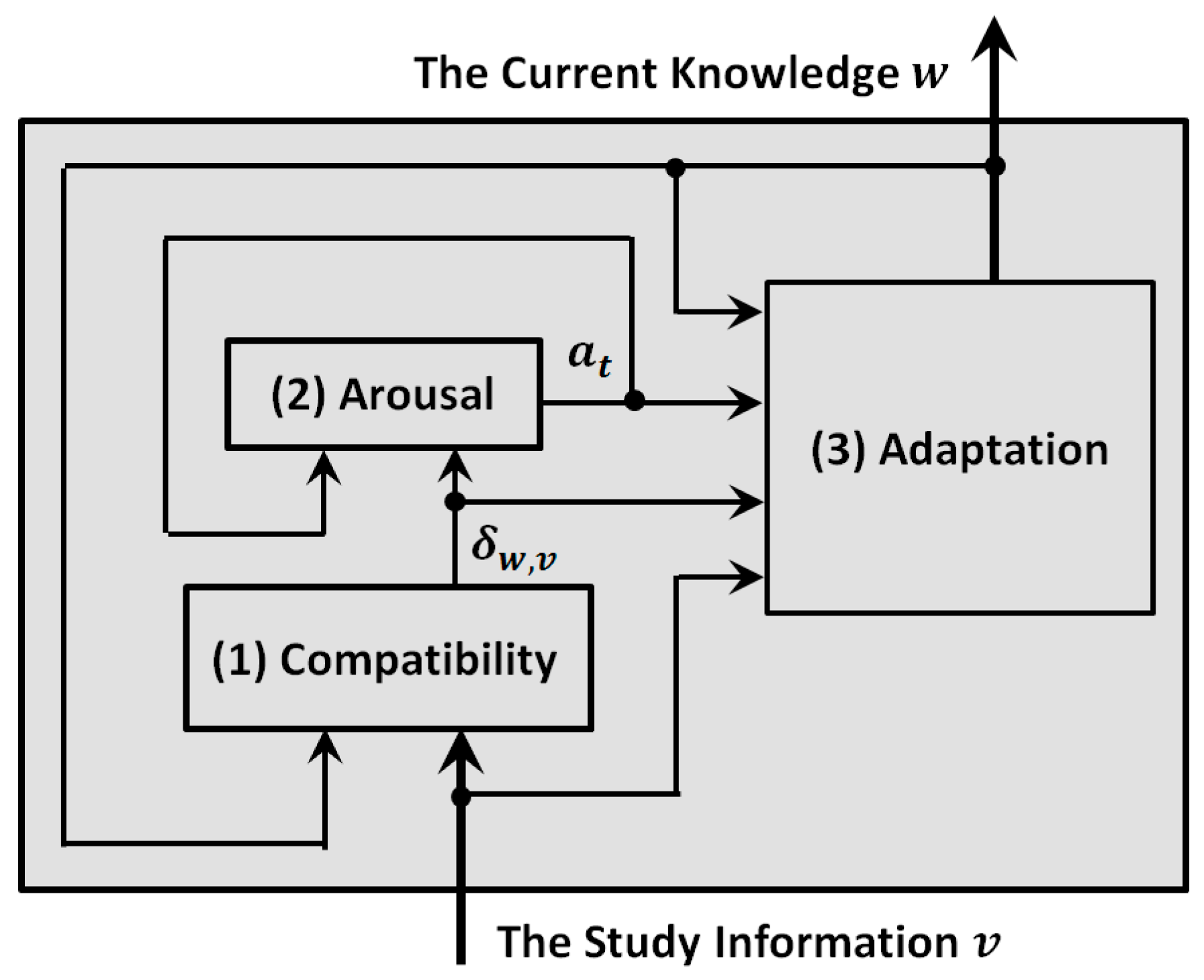
4. Solving (18) and (22) Using a Participatory Searching Algorithm (PSA)

The two proposed RBL methods both required solving a constrained optimization problem for accomplishing the RBL task. In particular, the OM approach needed to solve (18) for the translation vector and rotation matrix, while for the TM algorithm, the problem in (22) had to be solved to obtain the initial sensor position estimates in the current frame. In this work, we adopted the participatory search algorithm (PSA), an emerging population-based heuristic search algorithm, to find the optimal solutions to (18) and (22). The PSA was motivated by the participatory learning model proposed in [24,32].
The participatory learning diagram mainly consisted of the following three steps (see Figure 2), emulating the general learning process:
Step 1. Calculate the compatibility degree δ w , v between the current knowledge w ( t ) and learning information v ( t ) for the t -th iteration using
δ w , v ( t ) = 1 n = 1 N | w n ( t ) v n ( t ) | / N ,
where N is the dimensionality of the unknowns. In this work, N was equal to 6 for the problem in (18), and v 1 , , v 6 represented the elements in [ x , y , z , ϕ , φ , ψ ] . On the other hand, N was equal to K when solving (22), and v 1 , , v K were indeed y 1 , , y K .
Step 2. Update the arousal index a t based on the compatibility degree via
a t + 1 = ( 1 β ) a t + β ( 1 δ w , v ) ,
where the rate of the arousal change β ( 0 , 1 ) is a uniformly distributed random variable. The lower compatibility degree between the current knowledge and learning information was, the less confident the learning system was in the current knowledge, which led to an increased arousal index.
Step 3. Modify the current knowledge based on the compatibility degree, arousal index, the current knowledge, and the incoming information via
w ( t + 1 ) = w ( t ) + α δ w , v 1 a t + 1 [ w ( t ) v ( t ) ] ,
where the uniform random number α ( 0 , 1 ) is the basic learning rate.
The PSA algorithm followed the participatory learning paradigm presented above, and it carried out four processing stages [24], namely Pairing, Selection, Recombination, and Mutation, which are summarized in Algorithm 1. Essentially, the current population and current best individual took the role of the current knowledge in the participatory learning paradigm, while the newly produced population can be considered as the new knowledge.
The Paring operation aimed at finding each individual’s most similar mate according to (36). This encouraged that Selection and Recombination were performed between mates, from which good offspring were more likely to be produced to improve performance. The output of PSA was the individual leading to the maximum value of the associated objective function (see (17) and (21)).
Algorithm 1 Participatory Search Algorithm (PSA)
  Initialization: Randomly set v b e s t in the restricted area; a t = 0 ; t = 0 ; f is the fitness (objective) function.
  do
  Randomly generate M individuals v 1 , , v M in the restricted area and form M + 1 individuals: v = [ v 1 , , v M , v b e s t ] . Each individual contains N unknowns;
  Update v b e s t with argmax r f ( r ) ,   r v ;
  Pairing:
  For each individual v m , find its mate v m by
   v m = argmax r δ r , v m ,   r v , r v m ;
  Let v = [ v 1 , , v M + 1 ] ;
  for m = 1 : M
  Selection:
  if δ v m , v b e s t > δ v m , v b e s t then p m s = v m ;
  else p m s = v m ; end if
  Recombination:
  Choose α , β ( 0 , 1 ) randomly;
  Compute a t + 1 = ( 1 β ) a t + β [ 1 δ v m , v m ] ;
  Generate offspring p m r = v m + α δ v m , v m 1 a t + 1 ( v m v m ) ;
  Mutation:
  Get p m t = v b e s t + α δ p m s , p m r 1 a t + 1 ( p m s p m r )
  if f ( p m t ) > f ( v b e s t ) then v b e s t = p m r ; end if
  if f ( p m s ) > f ( v b e s t ) then v b e s t = p m s ; end if
  end
   t = t + 1 ;
  while t < t m a x
  return v b e s t

5. Performance Evaluation

Simulations were conducted to evaluate the performance of the proposed two algorithms, namely the OM method and TM algorithm with refinement, both of which achieved the DoA-based RBL with a single base station. Instead of comparing against the ToA-based RBL schemes, we shall investigate the DoA-based RBL performance as a function of the size of the rigid target and the DoA measurement noise level. The existing TM method without the refinement process, which was developed in [23], was simulated as a benchmark technique. The CCRB derived in Section 2.2 was included as well for the purpose of comparison. It is well-known that the CCRB gives a lower bound on the estimation variance of all the unbiased estimators of deterministic parameters with equality constraints. It has been used extensively in localization literature because of its good prediction on the performance limit over a small noise region.

5.1. Simulation Setup

The simulation setup was as follows. The single BS was deployed at the origin. K = 4 wireless sensors were mounted on the rigid body to be localized. The topology information of the sensors was given in the sensor distance vector d = D · [ 1 , 1 , 1 , 2 , 2 , 2 ] T , which indicated that the sensors were distributed on the vertices of an isosceles trirectangular tetrahedron, and D denoted the size of the rigid body. As a result, the reference frame is given by
C = [ 0 1 0 0 0 0 0 0 1 0 0 1 ] · D .
In the simulation experiments performed in the next subsection, Section 5.2, we considered the scenarios where D was equal to 1, 1.5 and 2 m.
We set the true Euler angles φ , ϕ , and ψ to be 10°, 60°, and −25°, respectively, with respect to the reference frame. The associated rotation matrix Q is thus given by, according to (3),
Q = [ 0.4532 0.211 0.8660 0.5525 0.8290 0.087 0.700 0.5178 0.4924 ] .
We assumed a translation vector t = [ 6   6   2 ] T . Accordingly, the ground truth of current frame S of the rigid target will be generated through putting the specified values of t and Q into (1).
The noise of the DoA measurements from sensors in the current frame to the single BS, Δ α k and Δ β k , had the same noise standard deviation of σ degrees. The number of ensemble runs N I t e r was equal to 500. The estimation root mean squared error (RMSE) of a parameter X was computed using:
RMSE ( X ) = 1 N I t e r n = 1 N I t e r | | X X ^ n | | 2 ,
where X ^ n was the estimate of X in the n -th ensemble run. The Euclidean norm was used when X was a vector, and the Frobenius norm applied when X was a matrix. The estimation bias of X was obtained by:
Bias ( X ) = | | 1 N I t e r n = 1 N I t e r ( X X ^ n ) | | .

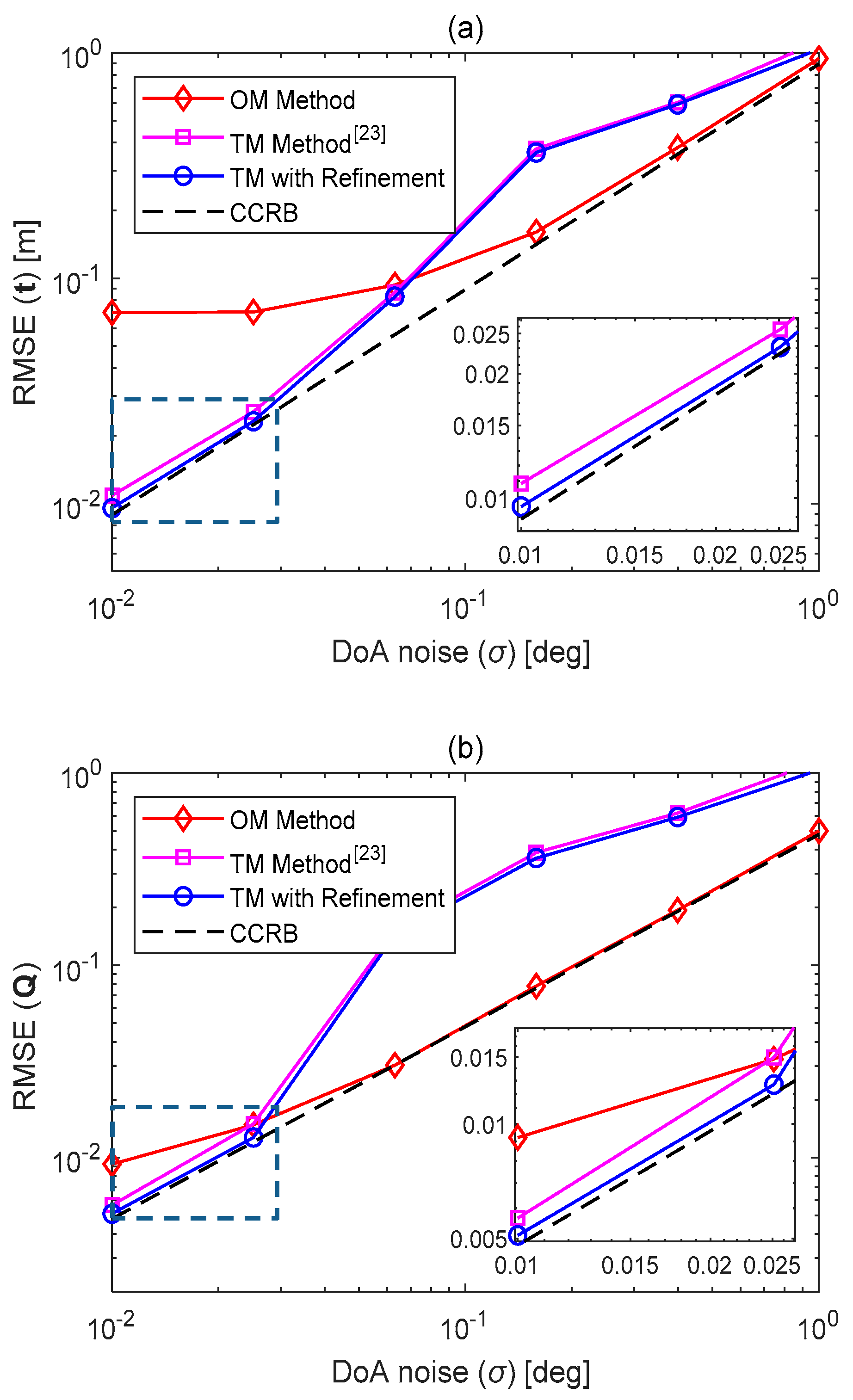
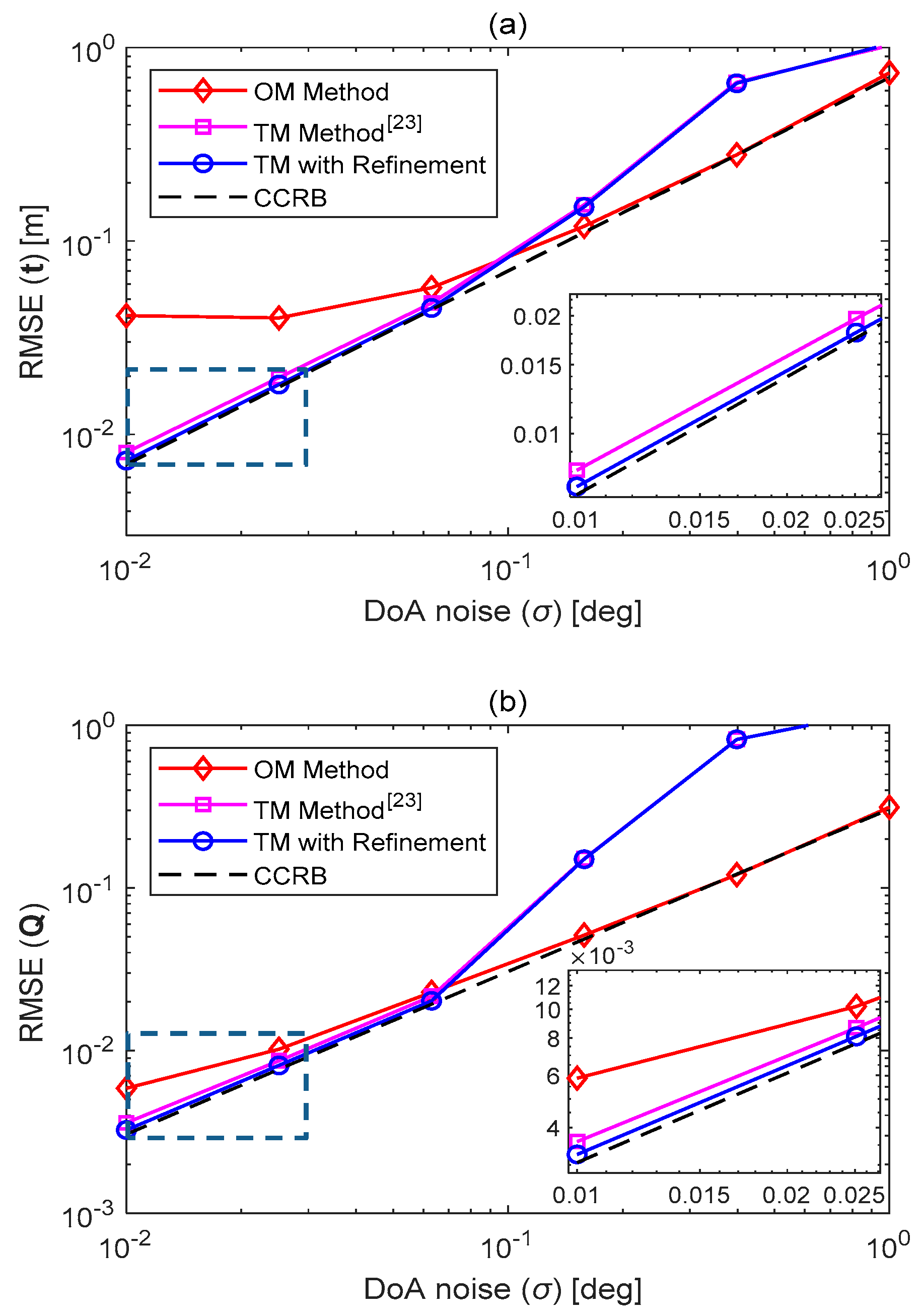
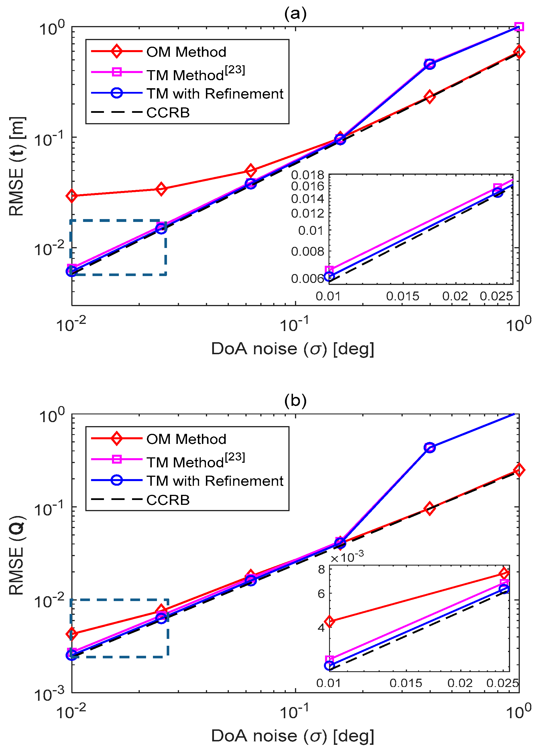
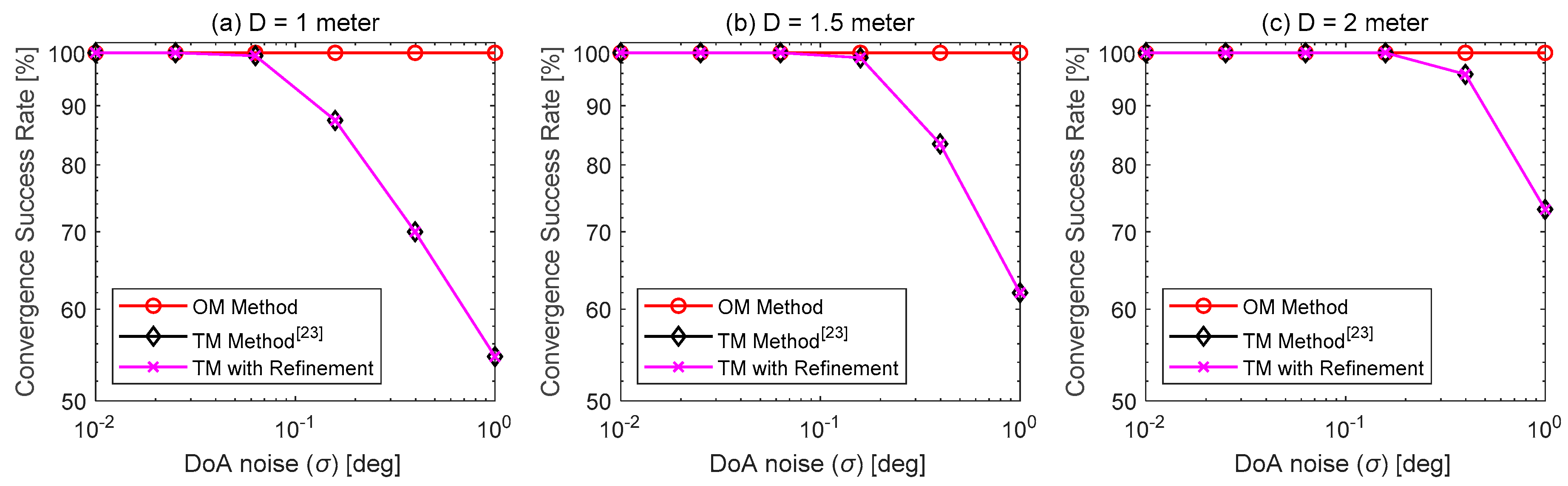
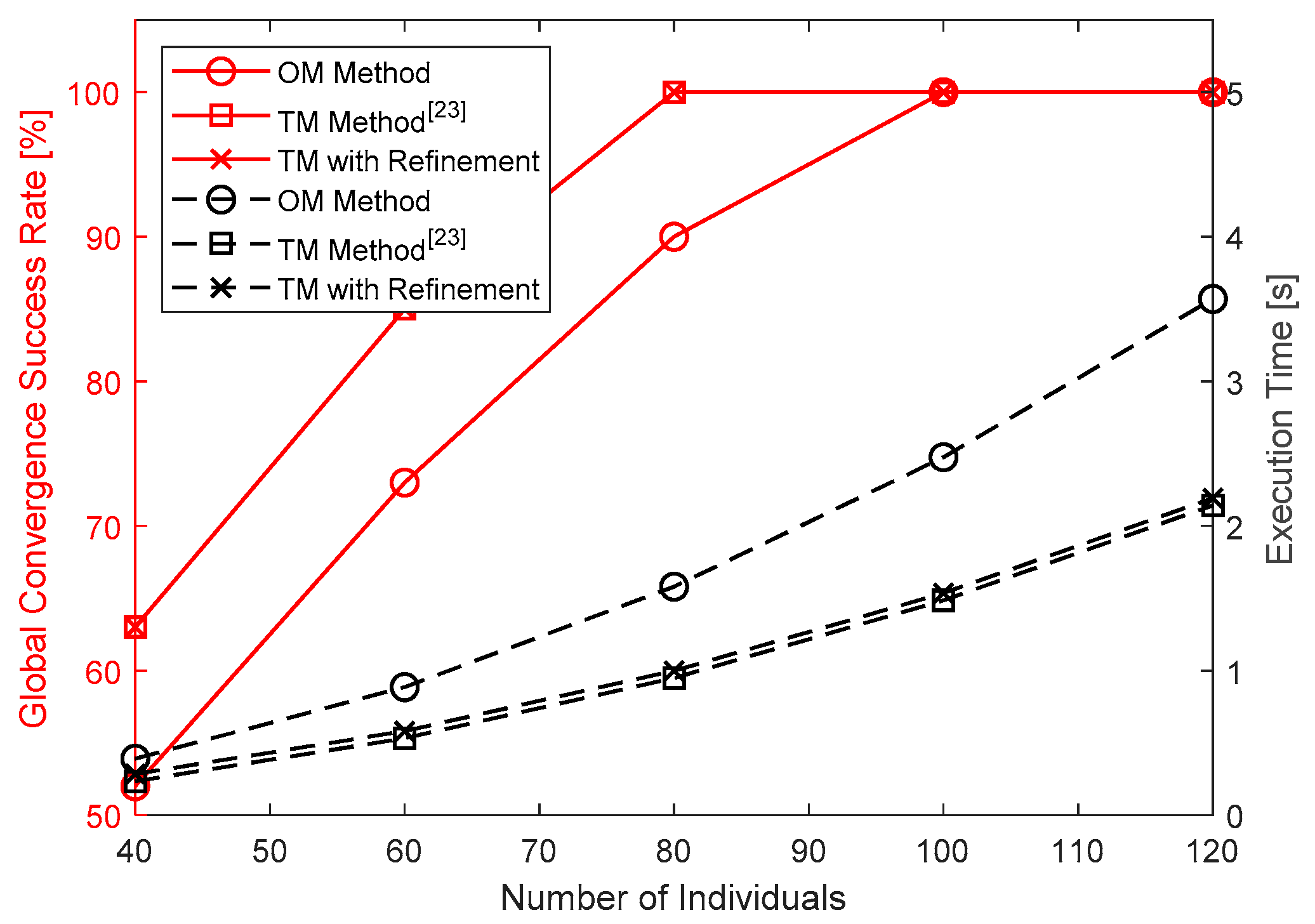
5.2. Simulation Results Evaluation

In Figure 3, Figure 4 and Figure 5, we plotted the RMSEs of the translation vector t (the location information of the rigid target) and the rotation matrix Q (the attitude information of the rigid target) estimates, when the sizes of the rigid target D were set to be 1, 1.5, and 2 m, and σ was equal to 10−2, 10−1.6, 10−1.2, 10−0.8, 10−0.4 and 1 degrees.
As we expected, the estimation RMSEs decreased as the DoA noise level reduced. In addition, increasing the size of the rigid target D enhanced RBL accuracy. The reason was that the difference between the DoAs from the wireless sensors increased with larger values of D , which mitigated the effect of DoA noise on estimation performance.
As shown in Figure 3, Figure 4 and Figure 5, under low DoA noise conditions, the two considered TM-based methods outperformed the OM-based algorithm. Meanwhile, we also observed from the ‘zoom-in’ windows in these figures that the proposed TM technique with WLS-based refinement achieved better RBL accuracy, and its performance was closer to the CCRB than that of the existing TM method in [23]. The level of performance improvement was more evident under smaller rigid body sizes and DoA noise levels. This enhancement mainly came from the improved sensor node positions resulting from the introduction of the additional processing stage, Stage 2, as shown in Table 1 where the positioned RMSEs of the wireless nodes in the current frame are provided. These results confirmed the effectiveness of the refinement stage.
When the DoA noise level became larger, the estimation performance of both the TM method from [23] and the proposed TM method with refinement exhibited apparent deviation from the CCRB, while the OM-based method offered an accuracy close to the CCRB. This was because the PSA algorithm adopted to solve the TM problem in (22) experienced a decrease in the global convergence rate. We illustrated this point in Figure 6, where the success rate of global convergence of the three methods in consideration was depicted as a function of the DoA measurement noise standard deviation σ and the rigid target size D. The proposed OM method achieved a global convergence rate very close to one, even when the rigid target size was D = 1 m and the DoA noise was as high as σ = 1 ° , which verified the robustness of the OM technique. On the other hand, the global convergence rates of the two TM techniques were sensitive to the decrease in the rigid target size and/or the increase in the DoA noises. The improved performance of the OM method was because it utilized 2 K = 8 DoA measurements for observation matching in (18), while with the TM methods, only K ( K 1 ) 2 = 6 sensor distances were used for topology matching in (22). Intuitively, the more measurements that were used, the more robust the RBL technique was to measurement noises.
Figure 7 shows the results for the estimation bias. The proposed TM method with refinement yielded the smallest bias in the case of low-level DoA measurement noise, while the proposed OM method performed better when measurement noise was large, which was expected from the obtained RMSE results.
Finally, analysis of the computational costs of the proposed techniques as conducted. The particle swarm optimization (PSO) algorithm was adopted for searching for the solution in the existing TM method [23]. Here, for fairness, we replaced it with PSA. This study was performed using MATLAB on a desktop with a 3.3 GHz CPU and 8GB RAM.
We illustrated the computational cost of the three RBL schemes in consideration when the DoA noise standard deviation was equal to σ = 10 1.6 degrees and the size of the rigid target was 1.5 m. We set the PSA iteration number to be 200, and the WLS iteration number in the TM method with refinement was 20. Figure 8 shows the global convergence success rate and execution time as a function of the number of individuals used in PSA.
To ensure convergence, the individual number should be at least 100. In this case, the execution time of the OM-based RBL method was around 2.5 s per ensemble run, and those of the TM-based RBL methods were around 1.5 s. The former technique had higher complexity because it had to jointly estimate six parameters ( x , y , z , ϕ , φ , ψ ), while the TM-based methods only needed to find four parameters. In addition, the newly introduced WLS-based refinement process did not introduce significant increases in the execution times of the TM-based RBL method.

6. Conclusions

In this paper, we considered the problem of DoA-based RBL adopting a single BS. The rigid target is mounted with wireless sensors, whose signal arriving angles can be acquired by the single BS equipped with an LSAA. The known topology information and the measured DoAs of the wireless sensors were fused to determine the position and orientation of the rigid target, with respect to the predetermined reference frame. We proposed two estimation approaches, namely the OM method and TM method with a refinement process. The PSA was adopted for the matching processes in both approaches to find the optimal parameters. We conducted simulations and compared their estimation accuracy with that of an existing benchmark, as well as the CCRB. Results show that the TM method with a refining process performed better in lower level noise conditions, while the OM method was more robust against higher level noise.

Author Contributions

B.Z. and L.Y. conceived and designed the experiments; B.Z. and S.Y. performed the experiments; X.Y., Y.K. and B.Z. analyzed the data; S.W. and L.A. contributed reagents/materials/analysis tools; B.Z. and L.Y. wrote the paper.

Funding

This work was supported in part by the National Natural Science Foundation of China (Grant No. 61703185), the 111 Project (B12018), Natural Science Foundation of Jiangsu Province (No. BK20180597), and the Jiangsu Key Construction Laboratory of IoT Application Technology (No. 18WXWL08).

Acknowledgments

We gratefully acknowledge the valuable cooperation of Sabbir Ahmed (Jiangnan University) in preparing this manuscript.

Conflicts of Interest

The authors declare no conflict of interest.

References

  1. Featherstone, R. Robot Dynamics Algorithms; Springer: Berlin/Heidelberg, Germany, 2014. [Google Scholar]
  2. From, P.J.; Gravdahl, J.T.; Pettersen, K.Y. Rigid Body Dynamics, Vehicle-Manipulator Systems; Springer: Berlin/Heidelberg, Germany, 2014; pp. 191–227. [Google Scholar]
  3. Garcia-Nieto, S.; Velasco-Carrau, J.; Paredes-Valles, F.; Salcedo, J.V.; Simarro, R. Motion Equations and Attitude Control in the Vertical Flight of a VTOL Bi-Rotor UAV. Electronics 2019, 8, 208. [Google Scholar] [CrossRef]
  4. Sauer, J.; Schömer, E. A Constraint-Based Approach to Rigid Body Dynamics for Virtual Reality Applications. In Proceedings of the ACM symposium on Virtual Reality Software and Technology, Taipei, Taiwan, 2–5 November 1998; pp. 153–162. [Google Scholar]
  5. Hua, M.D. Attitude estimation for accelerated vehicles using GPS/INS measurements. Control Eng. Pr. 2010, 18, 723–732. [Google Scholar] [CrossRef]
  6. Liu, C.; Yang, L.; Mihaylova, L. Dual-satellite source geolocation with time and frequency offsets and satellite location errors. In Proceedings of the 20th International Conference on Information Fusion (Fusion), Xi’an, China, 10–13 July 2017; pp. 1–8. [Google Scholar]
  7. Liu, L.; Zhang, X.; Chen, P. Compressed Sensing-Based DoA Estimation with Antenna Phase Errors. Electronics 2019, 8, 294. [Google Scholar] [CrossRef]
  8. Kim, Y.; Kim, N. An Enhanced 3D Positioning Scheme Exploiting Adaptive Pulse Selection for Indoor LOS Environments. Wirel. Pers. Commun. 2014, 77, 2537–2548. [Google Scholar] [CrossRef]
  9. Namvar, M.; Safaei, F. Adaptive Compensation of Gyro Bias in Rigid-Body Attitude Estimation Using a Single Vector Measurement. IEEE Trans. Autom. Control 2013, 58, 1816–1822. [Google Scholar] [CrossRef]
  10. Wu, Y.; Shi, W. On Calibration of Three-Axis Magnetometer. IEEE Sens. J. 2015, 15, 6424–6431. [Google Scholar] [CrossRef] [Green Version]
  11. Wu, Z.; Yao, M.; Ma, H.; Jia, W. Improving Accuracy of the Vehicle Attitude Estimation for Low-Cost INS/GPS Integration Aided by the GPS-Measured Course Angle. IEEE Trans. Intell. Transp. Syst. 2013, 14, 553–564. [Google Scholar] [CrossRef]
  12. Zhu, J.; Li, T.; Wang, J.; Hu, X.; Wu, M. Rate-gyro-integral constraint for ambiguity resolution in GNSS attitude determination applications. Sensors 2013, 13, 7979–7999. [Google Scholar] [CrossRef]
  13. Peng, H.M.; Chang, E.R.; Wang, L.S. Rotation method for direction finding via GPS carrier phases. IEEE Trans. Aerosp. Electron. Syst. 2000, 36, 72–84. [Google Scholar] [CrossRef]
  14. Natraj, A.; Ly, D.S.; Eynard, D.; Demonceaux, C.; Vasseur, P. Omnidirectional vision for UAV: Applications to attitude, motion and altitude estimation for day and night conditions. J. Intell. Robot. Syst. 2013, 69, 459–473. [Google Scholar] [CrossRef]
  15. Serra, P.; Cunha, R.; Hamel, T.; Cabecinhas, D.; Silvestre, C. Landing of a Quadrotor on a Moving Target Using Dynamic Image-Based Visual Servo Control. IEEE Trans. Robot. 2016, 32, 1524–1535. [Google Scholar] [CrossRef]
  16. Eggert, D.W.; Lorusso, A.; Fisher, R.B. Estimating 3-D Rigid Body Transformations: A Comparison of Four Major Algorithms. Mach. Vis. Appl. 1997, 9, 272–290. [Google Scholar] [CrossRef]
  17. Pizzo, A.; Chepuri, S.P.; Leus, G. Towards Multi-rigid Body Localization. In Proceedings of the IEEE International Conference on Acoustics, Speech and Signal Processing (ICASSP), Shanghai, China, 20–25 March 2016; pp. 3166–3170. [Google Scholar]
  18. Chepuri, S.P.; Leus, G.; van der Veen, A.-J. Rigid Body Localization Using Sensor Networks. IEEE Trans. Signal Process. 2014, 62, 4911–4924. [Google Scholar] [CrossRef]
  19. Chen, S.; Ho, K.C. Accurate Localization of A Rigid Body Using Multiple Sensors and Landmarks. IEEE Trans. Signal Process. 2015, 63, 6459–6472. [Google Scholar] [CrossRef]
  20. Jiang, J.; Wang, G.; Ho, K.C. Accurate Rigid Body Localization via Semi-definite Relaxation Using Range Measurements. IEEE Signal Process. Lett. 2018, 25, 378–382. [Google Scholar] [CrossRef]
  21. Jiang, J.; Wang, G.; Ho, K.C. Sensor Network-Based Rigid Body Localization via Semi-Definite Relaxation Using Arrival Time and Doppler Measurements. IEEE Trans. Wirel. Commun. 2019, 18, 1011–1025. [Google Scholar] [CrossRef]
  22. Zhou, B.; Jing, C.; Kim, Y. Joint ToA/AOA Positioning Scheme with IP-OFDM Systems. Wirel. Pers. Commun. 2014, 75, 261–271. [Google Scholar] [CrossRef]
  23. Zhou, B.; Ai, L.; Dong, X.; Yang, L. DoA-Based Rigid Body Localization Adopting Single Base Station. IEEE Commun. Lett. 2019, 23, 494–497. [Google Scholar] [CrossRef]
  24. Liu, Y.L.; Gomide, F. A Participatory Search Algorithm. In Evolutionary Intelligence; Springer: Berlin/Heidelberg, Germany, 2017. [Google Scholar]
  25. Diebel, J. Representing attitude: Euler angles, unit quaternions, and rotation vectors. Matrix 2006, 58, 15–16. [Google Scholar]
  26. Sun, M.; Yang, L.; Guo, F. Improving noisy sensor positions using accurate inter-sensor range measurements. Signal Process. 2014, 94, 138–143. [Google Scholar] [CrossRef]
  27. Gu, J.F.; Zhu, W.P.; Swamy, M.N.S. Joint 2-D DoA estimation via sparse L-shaped array. IEEE Trans. Signal Process. 2015, 63, 1171–1182. [Google Scholar] [CrossRef]
  28. Meng, D.; Wang, X.; Huang, M.; Shen, C.; Bi, G. Weighted Block Sparse Recovery Algorithm for High Resolution DoA Estimation with Unknown Mutual Coupling. Electronics 2018, 7, 217. [Google Scholar] [CrossRef]
  29. Kay, S.M. Fundamentals of Statistical Signal Processing: Estimation Theory; Prentice Hall: Upper Saddle River, NJ, USA, 1993. [Google Scholar]
  30. Stoica, P.; Ng, B.C. On the Cramér-Rao bound under parametric constraints. IEEE Signal Process. Lett. 1998, 5, 177–179. [Google Scholar] [CrossRef]
  31. Cox, T.; Cox, M. Multidimensional Scaling; CRC Press: Boca Raton, FL, USA, 2000. [Google Scholar]
  32. Yager, R.R. A model of participatory learning. IEEE Trans. Syst. Man Cybern. 1990, 20, 1229–1234. [Google Scholar] [CrossRef]
Figure 1. Direction of Arrival (DoA)-based rigid body localization (RBL) scheme in consideration.
Electronics 08 00622 g001
Figure 2. Diagram of the participatory learning mechanism.
Electronics 08 00622 g002
Figure 3. Comparison of root mean squared errors (RMSEs) of (a) the estimated translation vector and (b) the estimated rotation matrix, when D = 1 m. Note: OM = observation matching; TM = topology matching; and CCRB = constrained Cramér–Rao bound.
Electronics 08 00622 g003
Figure 4. Comparison of RMSEs of (a) the estimated translation vector and (b) the estimated rotation matrix, when D = 1.5 m.
Electronics 08 00622 g004
Figure 5. Comparison of RMSEs of (a) the estimated translation vector and (b) the estimated rotation matrix, when D = 2 m.
Electronics 08 00622 g005
Figure 6. Comparison of the global convergence success rate as a function of the rigid target size D and DoA noise standard deviation σ . (a) D = 1   m ; (b) D = 1.5   m ; (c) D = 2   m .
Electronics 08 00622 g006
Figure 7. Bias for (a) translation vector estimate and (b) rotation matrix estimate when D = 1.5 m.
Electronics 08 00622 g007
Figure 8. Comparison of the global convergence success rates and executed times as a function of the number of individuals used in the participatory searching algorithm (PSA).
Electronics 08 00622 g008
Table 1. Comparison of the positioned RMSEs of the wireless nodes.
Noise σ = 10 2   deg σ = 10 1.6   deg
Size
D = 1   m 11.3/8.7 (1.14 dB) 126.6/22.3 (0.77 dB)
D = 1.5   m 8.7/7.3 (0.76 dB)20.9/16.4 (1.05 dB)
D = 2   m 7.3/6.5 (0.50 dB)17.6/15.2 (0.64 dB)
1 Positioned RMSEs (in mm) of the existing TM/the proposed TM with refinement (improvement in dB).

