Machine Learning Prediction Approach to Enhance Congestion Control in 5G IoT Environment

Abstract

The 5G network is a next-generation wireless form of communication and the latest mobile technology. In practice, 5G utilizes the Internet of Things (IoT) to work in high-traffic networks with multiple nodes/sensors in an attempt to transmit their packets to a destination simultaneously, which is a characteristic of IoT applications. Due to this, 5G offers vast bandwidth, low delay, and extremely high data transfer speed. Thus, 5G presents opportunities and motivations for utilizing next-generation protocols, especially the stream control transmission protocol (SCTP). However, the congestion control mechanisms of the conventional SCTP negatively influence overall performance. Moreover, existing mechanisms contribute to reduce 5G and IoT performance. Thus, a new machine learning model based on a decision tree (DT) algorithm is proposed in this study to predict optimal enhancement of congestion control in the wireless sensors of 5G IoT networks. The model was implemented on a training dataset to determine the optimal parametric setting in a 5G environment. The dataset was used to train the machine learning model and enable the prediction of optimal alternatives that can enhance the performance of the congestion control approach. The DT approach can be used for other functions, especially prediction and classification. DT algorithms provide graphs that can be used by any user to understand the prediction approach. The DT C4.5 provided promising results, with more than 92% precision and recall.

1. Introduction

Wireless sensor networks have played a crucial role in communication in the past few decades due to their unique features (e.g., mobility and ease of connection), which make them a major carrier of data across networks [1,2,3]. Consequently, the communication revolution embraces various standard wireless networks. Numerous types of wireless networks exist, and mobile wireless communication is one of the most widespread because it offers high data bandwidth. Mobile wireless communication utilizes a transport layer to transfer data and launches a specific protocol for data transmission. The transport layer protocol uses a congestion control mechanism to ensure good network resource allocation, and the network operates optimally even when demands reach the maximum network resources and size. One of the most critical events of the transport layer protocol is congestion control over wireless networks. If this event is used in a mobile wireless communication platform such as 5G, and does not satisfy the requirements of the platform, then the performance of the wireless network will deteriorate.

Congestion control shortage is one of the main causes of the decrease in the lifetime and energy of wireless sensor network (WSN) nodes [4,5]. This decrease leads to many other issues, such as delay, packet loss, and bandwidth degradation [6]. Network resources include buffer size, queue size, throughput, link bandwidth, and packet loss of intercommunication between nodes [7]. Congestion control influences diverse applications, such as event-based, continuous sensing, query-driven, and hybrid applications [8]. Congestion control is applied in different protocols in the transport layer, such as the transmission control protocol (TCP) and stream control transmission protocol (SCTP) [9]. Many conditions, such as packet collisions, interference, channel contention, and buffer overflow, require congestion control [4], whereas slow links, buffer size shortage, and slow processors do not need congestion control [7].

Many attempts have been made to enhance—while increasing the pace of—congestion control mechanisms, such as the proposal of a scalable distributed cluster-based congestion control scheme. In this scheme, the nodes are grouped in many clusters, where each cluster estimates the optimal path through message exchange within the cluster. However, this process may result in extra overhead along with energy consumption for head nodes within clusters [10]. An optimal model for network load level was proposed based on 3-bit representation; the model produced good convergence results and effective bandwidth allocation [11]. Measures have also been proposed to address issues in resource allocation, bandwidth delay, queue size, and high throughput [12], and a set of parameters based on channel load has been developed for distributed congestion control [13]. A previous study proposed a new algorithm to maximize the utilization of a link in data networking as well as overcoming data loss when congestion occurs [14,15]. A machine learning approach was used to improve congestion control, and the approach produced a promising result for the practical and oracular measurements of path properties [16,17]. Another study developed a novel method (expert framework) to estimate the end-to-end round-trip time using a machine learning approach. The simulation of this expert framework based on machine learning could adapt to changes in round-trip time, thereby reducing the number of transmitted packets while increasing the throughput [18]. As a part of machine learning, clustering was used in congestion control for a vehicular ad-hoc network that included three parts, namely, detecting congestion, clustering messages, and controlling data congestion. Machine learning plays a vital role in improving congestion control [19,20].

The 5G environment is applied in many fields and utilized for many purposes, such as smart cities [21], e-Health [22], and environmental surveillance [23]. Many approaches have been applied to the 5G environment in order to enhance the network performance [24]. The machine learning approach is effective and widely applicable. Thus, it can be implemented with the conventional congestion control mechanism to satisfy the demands of 5G Internet of Things (IoT) nodes/sensors networks. The aim of applying the machine learning method to congestion control is to predict the optimal parametric setting and path to send/receive data. Finding the optimal node reduces data traffic and packet loss and improves throughput. In this work, a machine learning approach is utilized for prediction based on support vector regression using two parameters, namely, file transfer history and the measurement of simple path properties. This study presents a new methodology for improving the congestion control mechanism based on the machine learning decision tree (DT) approach.

The rest of this paper is organized as follows. Section 2 presents related work on machine learning utilization for network optimization and prediction, congestion control mechanisms, and studies regarding congestion control improvement. Section 3 explains the mathematical model of the proposed congestion control method. Section 4 discusses the experimental results and demonstrates the effect of specific performance factors and the use of DT prediction. Section 5 presents the conclusions and directions for future work.

2. Related Work

Regarding the approaches to congestion control in WSN IoT highlighted by many studies, Sangeetha et al. [25] proposed a reduction of energy and data loss because of congestion across the network. Mainly, the topology of sensor nodes is attuned periodically at a regular time interval and node degree in order to improve the power consumption of sensor nodes, the interference, and provide an energy-efficient congestion-aware routing technique for WSNs—namely, survivable path routing (SPR). IoT applications use this protocol in networks with high traffic, since multiple sources are simultaneously trying to send their packets to a destination, as shown by Elappila et al. [26]. Singh et al. [27] developed a new congestion control algorithm for WSNs, where the conventional algorithms had high power usage and high complexity, and obtained the optimal rate by retransmission with congestion control, using a simple Poisson process. The routing protocol to select the optimized route proposed by Shelke et al. [28], based on opportunistic theory and by integrating suitable sleep scheduling mechanisms in order to decrease congestion in the network, increases individual node life, the entire network lifetime, and decreases division in the network. Godoy et al. [29] investigated and analyzed the environments that lead to congestion of the communication channel based on node configuration parameters: transmission time intervals, data packet generation rate, and transmitter output power level.

The congestion control mechanism of the SCTP determines its performance in various environments. Many studies have mentioned that conventional SCTP congestion control algorithms over Long Term Evolution-Advanced (LTE-A) present poor performance in terms of various factors, such as congestion window size (cwnd), throughput (throu), and send/receive/lose packets. Thus, Najm et al. [30] proposed an improvement mechanism called IMP-SCTP for 4G networks based on multi-criteria decision making (MCDM). Meanwhile, Najm et al. [31] described the conventional SCTP congestion control mechanism over a high-bandwidth network such as 4G as having weak performance through a hands-on and systemic review related to SCTP congestion control. New techniques must be adopted to enhance the congestion control scheme. One of the most vital studies involved the improvement of the congestion control of TCP in wired/wireless networks by applying a supervised machine learning technique; the authors built an automatic loss classifier from a database obtained by simulations of random network topologies [32]. However, the simulation scenario was poor and simple. Furthermore, a fair and efficient distributed congestion control algorithm for tree-based communication in WSNs that seeks to adaptively assign a transmission rate to each node was developed as stated by Brahma et al. [33]. However, the validation process did not compare the proposed algorithm to a standard/traditional method or a related previous study. In research published by Jagannathan and Almeroth [34], the authors proposed a new model for multicast congestion control called TopoSense. However, a multicast sub-tree needed to be developed, and high congestion control at high rates was caused by dropping. Moreover, the link capacity calculation was poor, the interval size needed to be calculated, bursty traffic occurred, and control traffic needed to be minimized. Sunny et al. [5] proposed a generic controller that ensures the fair and efficient operation of Wireless Local Area Network (WLANs) with multiple co-channel access points, long-lived performance, TCP transfers in multi-AP WLAN, and improves performance issues of long-lived TCP transfers in multi-AP WLANs.

Subsequently, many studies have adopted the DT concept in networks for various applications. For example, Katuwal et al. [35] proposed new multiple-classifier systems for multi-class classification problems. The proposed model is a combination of DTs (random forest and oblique random forest) with an efficient neural network (random vector functional link network). The result of model evaluation on 65 multi-class datasets was better than those on medium- and large-sized datasets. The model experiment on the multi-class datasets produced good results, and the model could perform similarly on large- and medium-sized datasets. The model considers the problem of multi-class classification and provides the same training datasets for two-class datasets. The result of the proposed ensemble of classifiers was better than those of other classifiers. Furthermore, Gómez et al. [36] compared the performance of various ensemble algorithms based on DT and presented a new classifier. The computational capacity of small network devices was not a crucial limitation.

Hasan et al. [37] conducted a review of a machine-to-machine communication technology related to the system model architecture anticipated by diverse standards-developing organizations and prospective machine-to-machine communication challenges and their intended state-of-the-art solutions. Leng et al. [38] proposed a new system for solving the flow table congestion problem in a software-defined network (SDN) based on a DT algorithm (C4.5). C4.5 was used to compress the flow entries in the data flow table in order to reduce the flow matching cost and time. This machine-learning-based online process in the SDN that is the first model to utilize a DT with a flow table. Then, a new trend of localization based on adaptive cluster splitting and AP reselection was proposed; Liang et al. [39] presented a new fingerprint-based indoor wireless LAN that adopts adaptive cluster splitting and access point reflection. However, only received signal strength (RSS) RSS was considered for fingerprinting, a large area of wireless technologies was not applied, and many other factors were not considered (e.g., packet loss, information of channel state, queue size, throughput). Following this trend, research published by Liu and Wu [40] used the machine learning approach (random forest algorithm) to predict traffic congestion. Variables such as weather conditions, road quality, time period, and type of day were used to build the model. However, many other factors, such as time and type of day (holiday), influence traffic congestion, make the prediction easy, and eliminate the need for prediction.

Following the trend of models based on Bayesian neural networks, Park et al. [41] created a model based on a Bayesian neural network with gradient-boosted DTs to predict secondary incident occurrences. The model aims to reduce potential accidents by alerting drivers about events that cause accidents. However, similar to many other models, this model cannot be applied in real-time systems that predict secondary incidents because the model needs real parameters to train and build the prediction results. Following the trend of implementing methods for link quality estimation based on DT and support vector machine (SVM) to propose an improved route of data delivery over WSNs, Shu et al. [42] utilized two parameters for estimation—namely, receive signal strength and link quality indicator. DT was combined with SVM in this model because SVM can only handle problems with binary classification. For energy-saving solutions for data centers and network infrastructures, a solution that is not a base technique was proposed in [43]. Following the trend of using DTs, Soltani and Mutka [44] presented a scheme using DT cognitive routing to determine the optimal path for sending data over a mesh cognitive radio network. The model allows a node to select the best candidate after analyzing the result tree and eliminate choices that decrease the node gain. Mesh cognitive networks and cognitive routing fields require analysis and intensive research to determine the critical points.

Furthermore, Soltani and Mutka [44] used the DT approach to translate cognitive video routing in a dynamic radio network. Background induction was used from the ending branches to find the optimal path to the root node in order to receive and construct the sent video. Following the trend of using machine learning DT techniques, Adi et al. [45] built a model to prevent denial of service over the hypertext transfer protocol (HTTP2). SVM, DT, naïve Bayes, and JRip DT were used for feature selection to determine important factors that influence false alarms. Using machine learning, the results demonstrated that the model is better than other models. Stimpfling et al. [46] proposed a method based on the DT algorithm in order to overcome the drawback of memory access as well as the size of the data structure. DT is considered as the optimizing point in the model because it reduces the searching time. Furthermore, Singh et al. [47] presented a new model to predict the noise of vehicular traffic. Four methods were used to build the model: DT, neural network, random forest, and the generalized linear model. The authors found that the random forest DT approach produced better prediction results than the other methods. To improve decryption efficiency over vehicular ad-hoc networks, Xia et al. [48] proposed a delegation scheme (CP-ABE) based on DT. DT was used to optimize the joined factors utilized for estimating the overhead of vehicle decryption. The results showed that DT had higher accuracy and precision than SVM and K-nearest neighbor and was thus the best choice for prediction.

The authors of the botnet attacker detector in SDNs [49] deployed a machine learning method regardless of the packet payload reading, but the stats plan required extensive computation. Wu et al. [50] presented a scalable machine learning (ML) approach that detects and predicts video freezes online by using features extracted from network-based monitoring data; the proposed scheme determines discriminative features based on multi-scale windows by using the criterion of information gain (IG), but requests of audio segments are ignored, user interactivity is restricted, the cache between the delivery nodes and the video player is ignored, and the segment length is fixed. Chen et al. [51] presented an online data model for traffic condition prediction that is based on online open data by using DT and SVM; however, the model selected to predict a 30 min traffic condition and the former two services exceeded the set value. Abar et al. [52] predicted the quality of experience based on full-reference parameters Structural Similarity Index (SSIM) and Video Quality Model. (VQM), but they did not explain why k = 9 in a random forest was the best.

Many studies have focused on network security by using the DT concept. For example, Pham and Yeo [53] proposed a secure and flexible framework for vehicles to manage trust and privacy, but the applied flexible recognition was unclear. Following the trends of reducing the amount of data transfer from smart meters, Mohamed et al. [54] presented an adaptive framework for minimizing the amount of data transfer from smart meters, but the proposed framework did not clarify the effect of the number of model updates. Next, Kong, Zang, and Ma [17] proposed two machine learning schemes based on TCP congestion control for under-buffered bottleneck links in wired networks with a compromise loss predictor and reinforcement to achieve a better tradeoff of delay. However, the environment used was wired. Taherkhani and Pierre [19] proposed a localized and centralized data congestion control approach to control data congestion employed in roadside units at intersections. The proposed approach comprises three parts for controlling data congestion, detecting congestion, and clustering messages. Thus, the K-means machine learning method was proposed to detect data congestion in channels over a VANET. In research published by Fadlullah et al. [20], the authors emphasized and demonstrated the necessity of overviewing the scattering mechanisms on deep learning applications for several network traffic control features, the state-of-the-art deep learning architectures and algorithms related to network traffic control systems, and also the potential enablers of deep learning for network systems. However, this was without a perspective of 5G environment utilization. Furthermore, authors in [45,55] proposed techniques for detecting previously unknown attacks on networks by identifying attack features. However, the relevance of window size and the attacks were not presented clearly.

Most of the previous studies frequently used decision tree machine learning to improve the network status without considering congestion control mechanisms over the recent environments (specifically the 5G IoT environment), even though DT presents a tree-based graph for prediction and classification. Therefore, DT should be developed for the prediction of the optimal congestion control mechanism among current congestion control transport protocol mechanisms in the 5G IoT environment. Despite these proposed methods, most studies only implemented machine learning capabilities in classifiers to improve network status without considering the current mechanisms required to adapt to new environments, such as advanced 4G and 5G, which could improve throughput and reduce end-to-end delay. Thus, 5G and the Internet of Things (IoT) represent a new era of applications and infrastructures that require the use of current mechanisms and protocols. Adapting to new environments is challenging in 5G, IoT, and current transport protocol mechanisms because transported protocols comprise the core of networks, which have unique characteristics compared with other protocols in mobile communication. The SCTP was introduced as the next-generation transport protocol to facilitate traffic in a way superior to conventional TCP and User Datagram Protocol (UDP). However, standard SCTP, TCP, and other transport protocols must be modified to suit the 5G environment. For these reasons, rapid response and reduced latency should be considered when improving a congestion control mechanism within 5G IoT networks. A demonstration of new approaches to overcome the limitation of current mechanisms should be considered to score the evaluation metrics of prediction and select the optimal techniques for congestion control as a means of achieving improved WSN performance in adjusting transport protocols for the improved support of 5G IoT environments.

The purpose of this work was to develop a new method for the prediction of congestion control mechanisms to adapt to 5G and evaluate the performance factors according to the machine learning capabilities for the SCTP. An analysis of the literature indicated several parameters for assessment/evaluation or utilization as evaluation metrics. However, in this research, we used the DT concept of machine learning capabilities during the development phase to predict the best I-cwnd for selecting the optimal threshold to adapt the SCTP to 5G IoT.

3. Proposed Congestion Control Prediction Approach

The congestion control algorithm is the essential mechanism of the SCTP and functions through the transport layer. Many tasks, comprising the transmitting and drawing of messages, error detection, and the retrieval of misplaced messages, can be achieved provided that the SCTP engages throughout this layer. These functions are adjusted to the obtainable utilization of the network. The number of terminals required to accomplish these functions is examined precisely as a result of the terminals-area-used units.

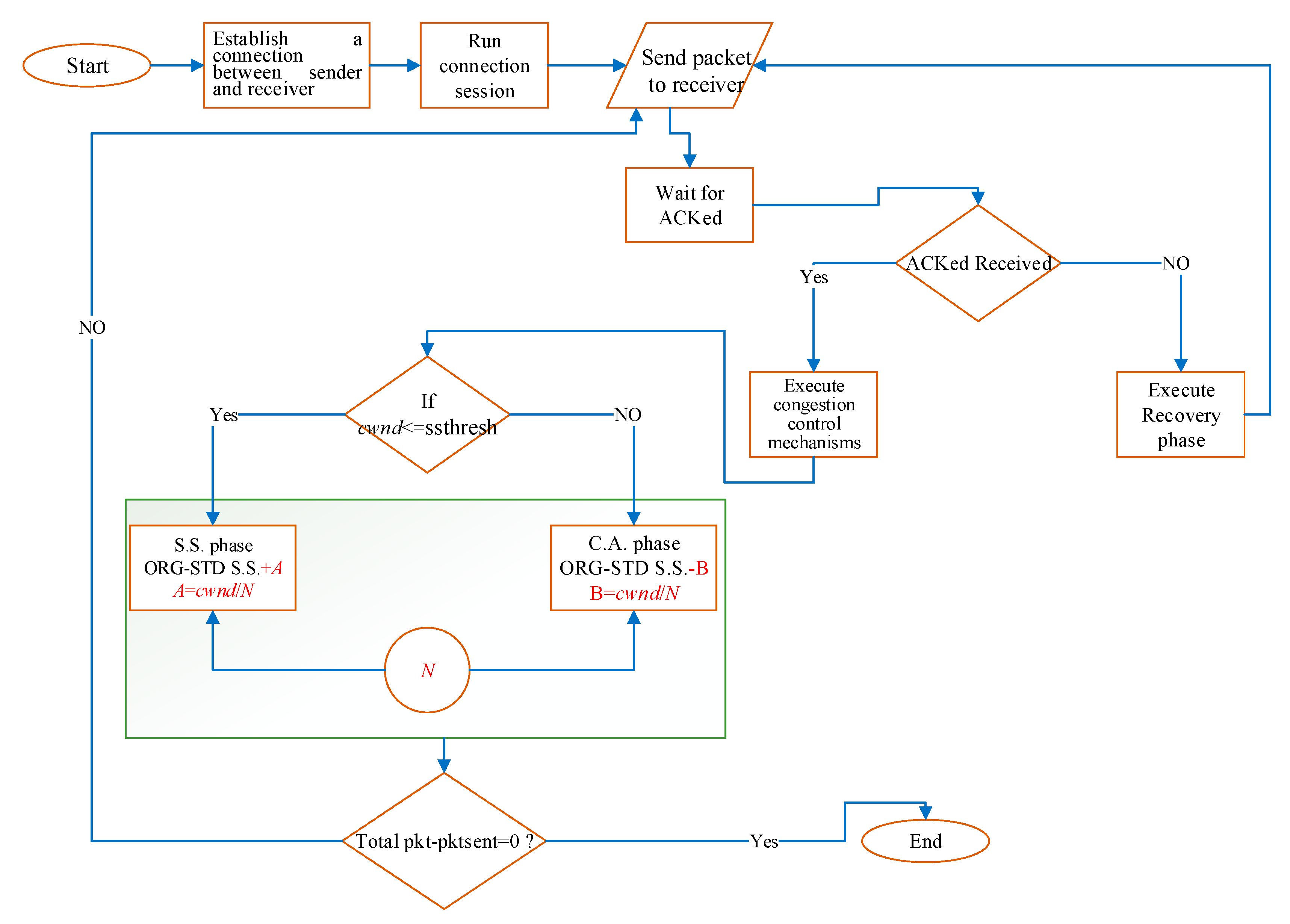
In the data transportation method, a transmitter must be linked to a recipient. The transmitter institutes a connection with a particular endpoint. It transmits the initial message and waits for acknowledgement (ACKed) to observe cwnd and ssthresh. When the recipient sends ACKed to the transmitter, cwnd and ssthresh are identified. Hence, congestion control is accomplished. If the recipient does not conduct ACKed, then the retrieval of the misplaced phase is done. If cwnd is less than or adequate to ssthresh, then the slow-start phase is established. When cwnd is larger than ssthresh, the congestion avoidance phases are executed. This process continues until all messages are delivered.

3.1. Modeling and Mathematical Formulation

Conventional or original SCTP (ORG-SCTP) was simulated in a 5G IoT environment, and the results showed that $cwnd$ grew progressively in a linear manner. It was assumed that when $cwnd\le ssthresh$, $cwnd$ would subsequently grow apiece ACKed in accordance with a specific interval. The details of the derived model and the visualization of the mathematical construction are mentioned in [30].

3.1.1. Enhanced Slow-Start

As data transmission begins, the phase of enhanced Slow-Start (S.S.) is initiated after a long period or under anonymous conditions. During this, the SCTP starts searching the whole network to estimate the capacity of the available bandwidth. To prevent the mechanisms which exceed the available resources, ssthresh is considered as the indicator to show the available bandwidth. The phase of slow-start can be detected by a retransmit timer and occurs after the reform of packet loss. When the cwnd is less than or equal to ssthresh, the cwnd will be increased after each acknowledgment. Therefore, the cwnd value will be increased exponentially. In this phase, the sender should not exceed the permitted demands by the algorithm. The following description shows the exponential enhancement of slow-start:

$$cwnd=cwnd+z,$$

where z can be considered as either the path maximum transmission unit (PMTU) of the destination or previous outstanding data chunk(s) acknowledged (data ACKed). PMTU is the destination PMTU and ACKed is the total size of chunks of the previous outstanding acknowledged data [45,46,47].

The standard equation of slow-start is shown as follows:

$$\mathsf{\Delta }cwnd slow start=min\left(Data acked,PMTU\right),$$

(1)

where the proposed equation of slow-start is written as follows:

$$\mathsf{\Delta }cwnd slow start = min\left(Data ACKed,PMTU\right)+A, where A=\frac{cwnd}{I}.$$

(2)

The parameter I is an integer that ranges from 1 to 100, determined depending on several performance factors. These factors are: number of packets received per period, number of sent packets per time unit, congestion window, number of dropped packets, and network throughput. The selection process intends to find the factor with high effective performance that affects the congestion control mechanism. The optimal I is chosen by replacing the value of I with the proposed equation. The outcomes of the performance factors determine the best value of I. The ideal outcome is determined as follows: maximum congestion window, maximum utilization of queue size, maximum number of received and sent packets, maximum throughput, and least packet loss. When the value of I exceeds 9, the packet loss will be aggravated. The queue size is affected by this occurrence. Based on these considerations, the outcomes of the performance factor, and the experimental results, the value of I ranges from 1 to 100 in enhanced slow-start.

3.1.2. Enhanced Congestion Avoidance

The establishment of Congestion Avoidance (C.A.) enhancement occurs when either the cwnd value or the amount of transmitted data exceeds the threshold. Thus, the congestion avoidance will enhance cwnd by 1 × MTU per round-trip time (RTT) when cwnd > ssthresh. The sender has either the transmitted data which is greater than the outstanding amount to the transport address or the cwnd value. The congestion avoidance mechanism works simultaneously with slow-start since cwnd is always compared with ssthresh. When the cwnd is less than or equal to ssthresh, the slow-start will be established; otherwise, the congestion avoidance phase is predominant. However, the interaction among these phases occurs especially when cwnd routes are varied in order to be occupied by particular phases. The PMTU is measured by the PMTU of the destination for each one multiplied by MTU per RTT, when cwnd > ssthresh [54,55,56,57,58].

The standard equation of congestion avoidance is written as:

$$\mathsf{\Delta }cwnd CA = \left(1 \times PMTU per RTT\right),$$

(3)

where the proposed equation of congestion avoidance is expressed as:

$$\mathsf{\Delta }cwnd CA = \left(1 \times PMTU per RTT\right)-B, where B \ne 0 and B =\frac{cwnd}{I}.$$

(4)

The proposed congestion avoidance equation subtracts B based on the value of I and the selected mechanism discussed previously. Congestion avoidance reduction to this amount can accelerate the congestion control process instead of slowing it down, as in the standard congestion avoidance equation. Furthermore, this decrease in congestion avoidance and the increase in slow-start can refine and optimize the congestion control of SCTP [56,59,60]. Thus, as explained previously, the proposed congestion avoidance equation should be converted into a non-homogeneous equation after undergoing the total average change.

3.2. Development Phase

This research discusses the improved SCTP (IMP-SCTP) congestion control mechanism of sensors in the 5G IoT environment. To achieve the third objective, improved slow-start and congestion avoidance techniques must be implemented. The improved approaches were used to solve the limitation of conventional congestion control in the 5G IoT environment. Various development processes were applied to create the final shape of IMP-SCTP based on an improved congestion control mechanism that uses DT capabilities. Two-stage testing with different scopes was implemented to develop IMP-SCTP. In the first stage, IMP-SCTP congestion control provided optimal window management according to the best I-selection. In the second stage, I-selection was led by DT. The evaluation criteria of DT techniques were queue size, throughput, packet loss, and cwnd. The improved approaches implement optimal window management through congestion avoidance and slow-start mechanisms, as shown in Figure 1.

At this point, all possible experiments, including related scenarios, have been covered and presented. Figure 1 depicts the stages of the IMP-SCTP congestion control mechanism. Based on these stages, two experiments were designed and developed. The details of these experiments are discussed in the next section. The improved mechanisms of congestion control utilize adapted approaches associated with slow-start and congestion avoidance mechanisms. Figure 2 demonstrates the processes of the proposed approaches and clarifies that each step relates to the congestion control model of the improved SCTP. To achieve the optimal I value, a machine learning approach is applied using C4.5, which is an algorithm utilized to accomplish DT that was proposed by Quinlan in 1970 [61]. J48 is an open-source implementation of the C4.5 algorithm. Thus, J48 obtains the optimal alternative and predicts the new optimal alternative based on the training table, which consists of a composite of specific performance factors. J48 generates a DT through the following steps.

3.3. Preparing the Training Dataset

The first stage involves preparing a dataset for the model to implement the model with a machine learning approach. C4.5 is used to generate a DT, which requires the feeding of a dataset to predict which I value exhibits the best performance and substitute it into the improved congestion control mechanism. The dataset was constructed from a specific set of performance factors and utilizes four performance factors, namely, cwnd, throughput (throu), queue size (que), and packet loss (pkt loss). The model aims to rank and predict optimal alternatives. In our case, I is a number ranging from 1 to 100 that denotes the substitutes to be classified. Thus, to select the utmost influential performance operators that affect the mechanisms of congestion control, the optimal I was determined by exchanging I into the improved approaches. The optimal I is based on the conduct of the performance metrics. The best performance is indicated by the maximization of throu, cwnd, que, number of pkt sent and received, and minimized pkt loss. However, once I-cwnd surpassed the values of 9 to 25, there was increased packet loss. This appearance aggravated queue size utilization. The optimization and prediction processes apply the rules accordingly. The following rule examines the optimal I based on an equation in which the supplied dataset is in the range of 1 to 100, and each represents an alternative related to its own (cwnd, throu, que, and pktloss).

The rule condition is built based on the IF statement below:

$$\begin{gathered} IF\{\left(\left(CWND>\overline{cwnd}\right) and \left(Throu>\overline{Throu}\right) and \left(Que> \overline{Que}\right) and (Pktloss \\ <\overline{Pkt loss})), then Optimal=“O”, else Optimal=“N”\right\}. \end{gathered}$$

(5)

The classifier rule indicates that all examined alternatives of the table categorized by Equation (1) are optimal when they satisfy the condition; that is, each true alternative is optimal (or “O”). Otherwise, it is not optimal (or “N”) because it does not achieve the effect threshold of the best performance based on the selected factors. The classified optimal alternatives that establish the DT preparation are shown in

Table 1. Classified optimal alternatives. CWND: congestion window size; O: optimal; N: non-optimal.

N	CWND	Throughput	Queue Size	Packet Loss	Optimal
1	120	9,881,687	48424	209	N
.	.	.	.	.	.
.	.	.	.	.	O
.	.	.	.	.	.
100	cwnd	throu	que	pkt loss	N

.

3.3.1. Applying the Machine Learning Approach

This phase of model implementation generates J48. Different machine learning approaches (e.g., clustering) are used in many fields for applications such as enhancing the performance of network nodes using clustering [19] and classifying the academic performance of students [62]. Compared with other data mining approaches, the DT approach plays numerous roles. The DT approach, as a part of machine learning [63], shows promising performance according to previous studies [64,65,66] that applied the approach in numerous fields, including medicine [67,68,69], e-government [70], wireless sensor networking [71], mobile authentication systems [72,73], and intrusion detection [57,74]. The DT algorithm builds an oriented tree graph based on training data for classification and regression. The tree graph comprises the root node, which branches to a subtree and ends with a leaf node. The path from the root to the leaf node passes through nodes that represent the attributes of the dataset. This path can be considered for the prediction of future cases. IF condition statements are used to build and translate the resulting tree [75]. DT is a robust and convenient machine learning approach that can be utilized in knowledge discovery to find hidden patterns in small and large datasets. Creating a tree involves three stages: construction, computation of information gain, and pruning. The construction stage includes the following basic steps [76,77]:

• Verify if all issues belong to the same class. Thus, a tree is a leaf that is labeled according to class.
• Compute the information gain and the information for a piece of the attribute.
• On the basis of the present selection criterion, locate the optimal splitting attribute.

The calculated information gain of entropy is used. Entropy is the measure of the uncertainty of a random variable. The entropy of Q is measured as follows:

$$Entropy\left(q\right)=-{{\displaystyle \sum }}_{i=1}^n\frac{\left|qi\right|}{\left|q\right|}log\left(\frac{\left|qi\right|}{\left|q\right|}\right),$$

(6)

where the conditional entropy is

$$Entropy\left(i|q\right)=-{{\displaystyle \sum }}_{i=1}^n\frac{\left|qi\right|}{\left|q\right|}log\left(\frac{\left|qi\right|}{\left|q\right|}\right),$$

(7)

where information gain is calculated as

$$Gain\left(q,i\right)=Entropy\left(p-Entropy\left(i|q\right)\right).$$

(8)

If the split is based on high gain, then the resulting tree will be small and efficient. In the final stage, a pruning technique is implemented to address overfitting and outliers. Pruning is used to classify datasets with poorly defined instances. Pruning is made up of two types. Online pruning is performed during tree creation, and post-pruning is performed after tree creation. Pruning implementation is based on separate-and-conquer rule schema. For the separate and conquer technique for P instances, the pruning steps are presented in

Table 2. Pruning algorithm steps.

Sequence	Step
1	K: = empty set of rules
2	while not P is empty
3	k: = best single rule for P
4	K: = add k to P
5	remove those instances from P that are covered by k
6	return K

.

3.3.2. Model Evaluation

The following criteria were used to evaluate DT performance and determine if the model is suitable for prediction [61,65,68,78]. The true positive (TP) instances represent the correctly predicted cases. The TP rate can be calculated as:

$$T{P}_{rate}=\frac{TP}{TP+FN}*100.$$

(9)

The true negative (TN) instances represent the correct prediction of negative cases. The false positive (FP) instances represent the incorrect prediction of positive cases, whereas false negative (FN) instances represent the incorrect prediction of negative cases. The FP rate can be calculated as follows:

$$F{P}_{rate}=\frac{FP}{FP+TN}*100\%.$$

(10)

The recall criterion generally represents the same values of TP rate, and this criterion is used with precision to estimate the relevance percentage. Precision can be measured as follows:

$$Precision=\frac{TP}{TP+FP}*100\%.$$

(11)

DT provides several benefits to machine learning, and these include easy comprehension by the end user and capability to address various input data (e.g., numerical, textual, and nominal). It also possesses the capability to process erroneous datasets or missing values. DT achieves a crucial accomplishment through simple efforts, and is applicable and scalable over diverse platforms. General DT virtualization consists of many nodes—namely, root and leaf nodes—that characterize many classes. The check condition augmented inside the internal node that is applied to attributes is shown in Figure 3.

4. Performance Evaluation

In this section, we discuss the experiments we conducted using the millimeter-wave (mmWave) model in the network simulator ns-3 [79,80] to evaluate the performance of the proposed DT in predicting the optimal parametric settings of sensors’ transport protocols over 5G IoT. In the evaluation of the improved SCTP IMP-SCTP versus ORG-SCTP, we specifically focused on two parts, namely, the setup for machine learning and the simulation results. We also compared the findings with those of state-of-the-art DTs and predictions of optimal sensors’ SCTP congestion control mechanisms over 5G IoT. We conducted a paired-sample t-test to show the significant variance between standard mechanism results and those of improved congestion control approaches.

4.1. Simulation Setup

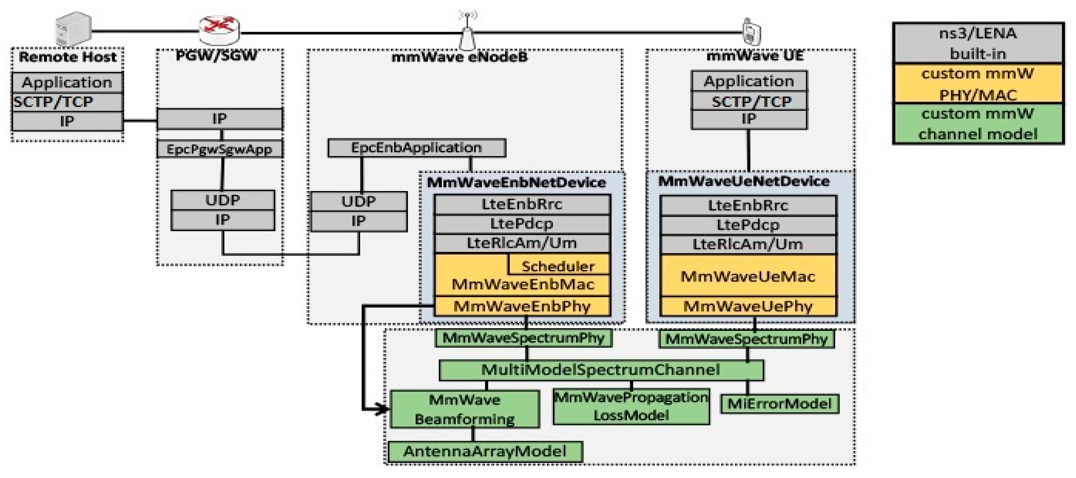
We employed the mmWave ns–3 module and mmWave protocols to evaluate network protocols, such as TCP and SCTP throughout the 5G mmWave environment. The attributes were configured accordingly as needed in the simulation. The details of attributes concerning the mmWave are found in the file named “mmWaveAttributesList”, whereas the objects are illustrated in the file named “MmWaveHelper”, where the method is provided [79,80]. mmWave was stacked through ns-three endpoints that included “UEs” and “eNBs”. The UEs were connected to E-UTRAN Node B (eNB), where both TCP and SCTP generated traffic throughout connections. The bandwidth uplink was 500 Mbps, and the downlink was 1Gpbs where the “UEs” delay was 1 ms. Then, the message transmission unit (MTU) size was 1500 bytes and the chunk size was 1468 bytes. Next, each eNB was connected to a group of 20–30 UEs. The eNBs were linked to Serving Gateway (SGW) and the core gateway Packet Data Network Gateway (PGW), the bandwidth of the upload link was 5 Gbps, with 5 ms delay. Both bandwidth and delay for the download link had the same upload link. PGW was employed as an HTTP cache server. It was connected to the remote host over a bidirectional connection. The bandwidth connection was 10 Gbps with a 10 ms delay. The drop-tail was used for the queue management scheme and active queue management. The mmWave carrier frequency was 28 GHz, and the mmWave bandwidth was 1 GHz, as presented in Figure 4.

4.2. Machine Learning Implementation

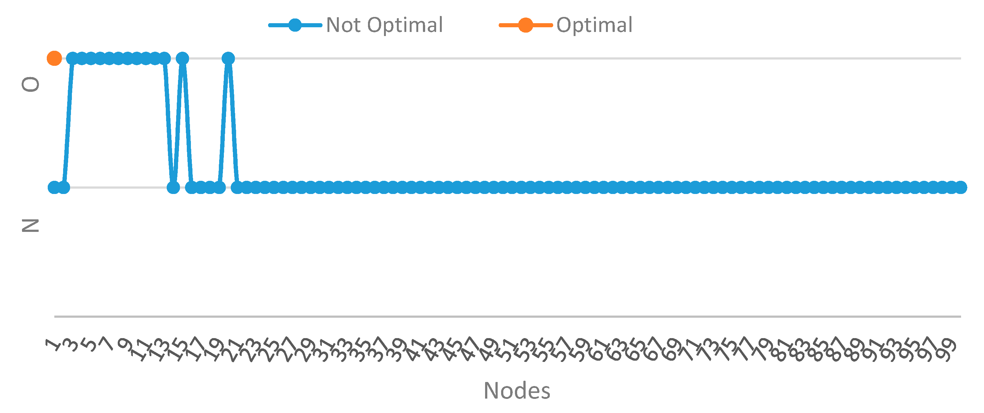
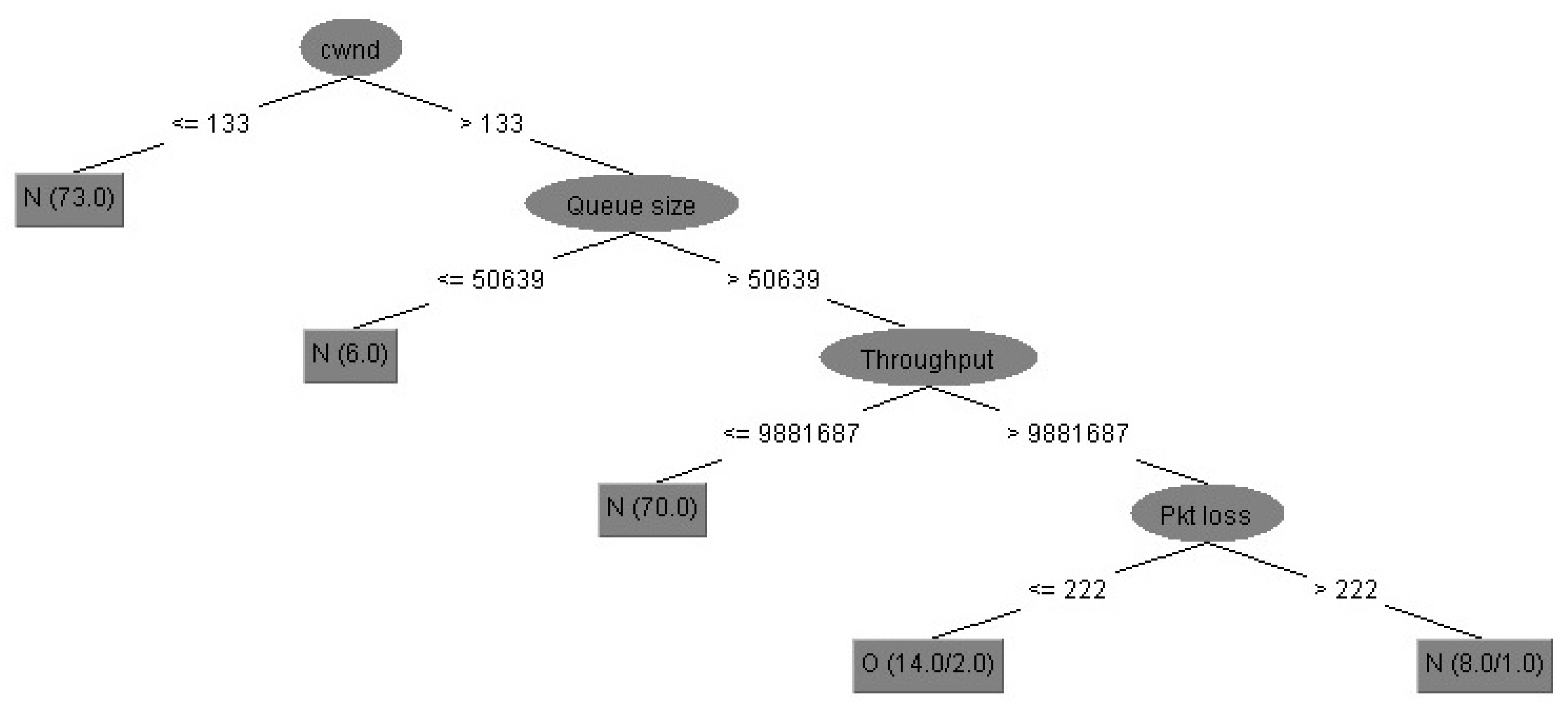
The model was implemented and tested using the Weka 3.8 tool. Weka 3.8 is an open-source machine learning tool that can be used to test and implement data mining tasks, such as prediction, analysis, and classification. Weka 3.8 offers wide flexibility in applying and listing predicted values. It enables the implementation of nearly all algorithms of data mining functions, such as clustering, association rules, regression, classification, and data pre-processing. The C4.5 DT algorithm is one of the commonly used algorithms for prediction and classification. C4.5 (J48) is used in Weka 3.8 for prediction and has proven accurate in different disciplines, such as education, medicine, sports, and economics. In our model, C4.5 was used to predict the optimal node in a 5G environment to help in congestion control. The first step in the model evaluation was DT/ML evaluation to determine if it covered all the training datasets and if the reader could visually determine the optimal node. Figure 5 shows the optimum alternatives whereas Figure 6 shows the result of the DT of congestion control based on the training dataset with predefined optimal nodes. The tree graph can provide the optimal node based on four factors (cwnd, que, throu, and pkt loss).

4.3. Effect of DT Prediction

The prediction concept is based on substituting a specific I-cwnd into the improved approaches. The selection of the optimal I is based on the conduct of the performance factors, where maximum cwnd, throu, and que represent the ideal outcome, in addition to a limited packet loss. Each I represents one of the I-alternative congestion control parameters. The branches below each node can define the conditions to determine the optimal and non-optimal nodes, where N refers to non-optimal and O refers to optimal in Figure 5.

The DT prediction in Figure 6 presents a tree graph after applying the J48 (C4.5) DT algorithm on the enhanced SCTP congestion control alternative. The root node is cwnd, and the arches represent the conditions of value comparison to determine the optimal node. The N leaf represents a non-optimal node, and optimal nodes are represented by “O”. If cwnd was less than or equal to 133, then the node was considered as N. Besides, the N represents the number of nodes that match the condition. If cwnd was greater than 133 and the queue size was less than or equal to 50,639, then six cases that matching this condition were considered as N nodes. If que was greater than 50,639 and throu was less than or equal to 9,881,687, then 70 cases were considered as N nodes. If throu was greater than 9,881,687 and pkt loss was less than or equal to 222, then the nodes would be considered as O.

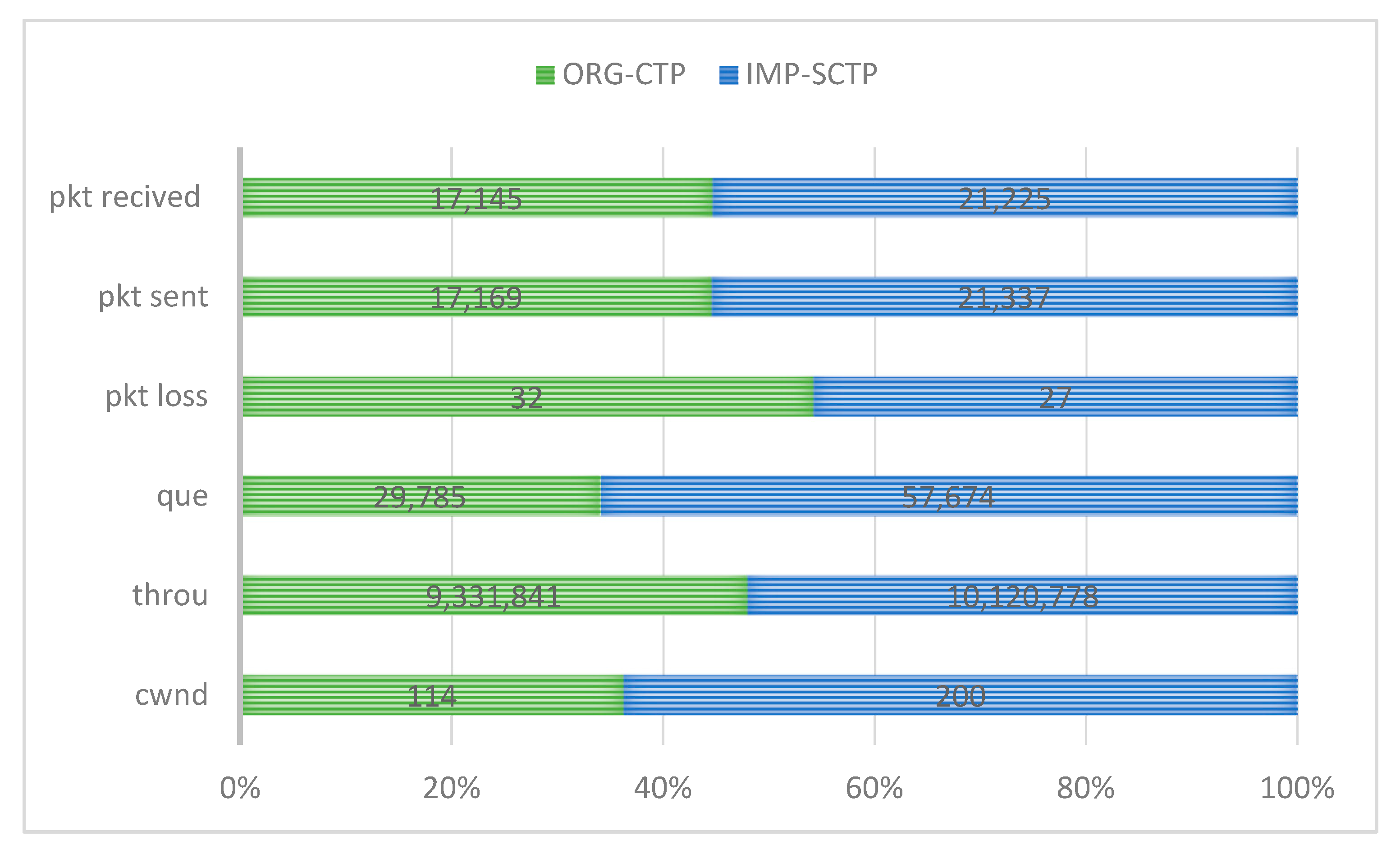
Fourteen cases satisfied this condition, and two cases were misclassified. In the final leaf branch, when the packet loss was less than 22, eight cases were considered non-optimal, and one case was misclassified. Based on this road map of DT and the IF–THEN statement used to find the optimal node, the best optimal nodes among all nodes were 3 and 4. I = 3 had a cwnd of 145, a throu of 9,905,462, a que of 53,788, and a pkt loss of 24. I = 4 had a cwnd of 200, a throu of 10,120,778, a que of 57,674, and a pkt loss of 27. These nodes satisfied all conditions and achieved the optimal factors that determine the optimal node among all nodes. The roadmap in the figure is helpful for manually detecting the optimal nodes by dropping the parameter readings on the tree.

After 80% of the dataset was divided into a training set and the remaining 20% as test set, the model was reevaluated to find the prediction margin in order to prove the accuracy of the DT prediction model. Figure 7 shows the margin score, which is a number that measures the accuracy of the predicted alternative, the prediction margin of each predicted node, and the accuracy measure of the prediction model. Margin scores range between 0 and 1; when the score is near 1 it means that the prediction is 100% accurate and when it nears 0 it indicates an incorrectly predicted alternative. Actual alternative (AA) represents whether an alternative is optimal or non-optimal. Predicted alternative (PA) represents the predicted case of the alternative after applying the DT algorithm. The figure demonstrates the accuracy of the DT prediction model, where the y-axis shows the margin scope of the prediction margin, and the x-axis represents the test alternatives by which the alternatives are shown as the actual alternatives and the predicted alternatives above them. These actual cases of alternatives were taken from the test set by which the alternatives were either O or N. The predicted alternatives represent the result of DT prediction by which the model predicted the alternative as either N or O. The prediction margin is a value that falls between 1 and −1. If the prediction value is 1, it means that the predicted value is 100% correct. When the value reaches 1, the prediction accuracy becomes perfect, and when the values reaches −1, it means that the predicted value is incorrect. The DT prediction model predicted the optimal node with 100% accuracy. The non-optimal alternatives were predicted with an average rate of 96%.

Table 3. DT evaluation. FP: false positive; PRC Area: area under the precision–recall curve; ROC Area: area under the receiver operating characteristic curve; TP: true positive.

Machine Learning	Algorithm	TP Rate	FP Rate	Precision	Recall	ROC Area	PRC Area
	C4.5	0.924	0.205	0.927	0.924	0.889	0.915
DT	RepTree	0.913	0.207	0.919	0.913	0.891	0.916
	Random Tree	0.913	0.207	0.919	0.913	0.891	0.916
Clustering	Simple K Means	0.891	0.018	0.939	0.891	0.937	0.923
	Hierarchical Clustering	0.857	0.870	0.752	0.857	0.527	0.771
Stacking	Zero + Decision Table	0.859	0.859	0.737	0.859	0.413	0.737

illustrates a comparison among three selected machine learning decision tree algorithms based on six performance criteria (TP rate, FP rate, precision, recall, receiver operating characteristic (ROC), and precision–recall curve (PRC)). The performance results of decision tree algorithms (C4.5, RepTree, and random tree) are presented. Additionally, in the clustering field of machine learning, the performance results simple K means and hierarchical clustering algorithms are listed, where the final section of the table presents the performance results of stacking, where many classifiers can be combined to predict the results.

The true positive (TP) rate represents the percentage of correct predictions as positive cases, and the false positive (FP) rate represents the percentage of incorrect predictions as positive cases of different selected classifiers and machine learning algorithms. Precision is the result of all correctly predicted cases divided by all cases. Recall or sensitivity is the result of correct predictions divided by the total positive cases. The area under the receiver operating characteristic curve (ROC) and area under the precision–recall curve (PRC) represent the general performance of the machine learning algorithm. While the TP rate is considered as optimal when its value is equal to 1, the optimal FP rate is reached when it is equal to zero. Moreover, the ideal value of precision and recall is 1.0, the ideal value of recall and precision is 1.0, where the worst value is 0. The area under the ROC curve represents the relationship between recall and specificity, where specificity represents the precision of truly predicted cases as negative when they are negative. Area under the PRC is where the relationship between recall and precision is estimated. Higher rates of ROC and PRC represent a better classifier.

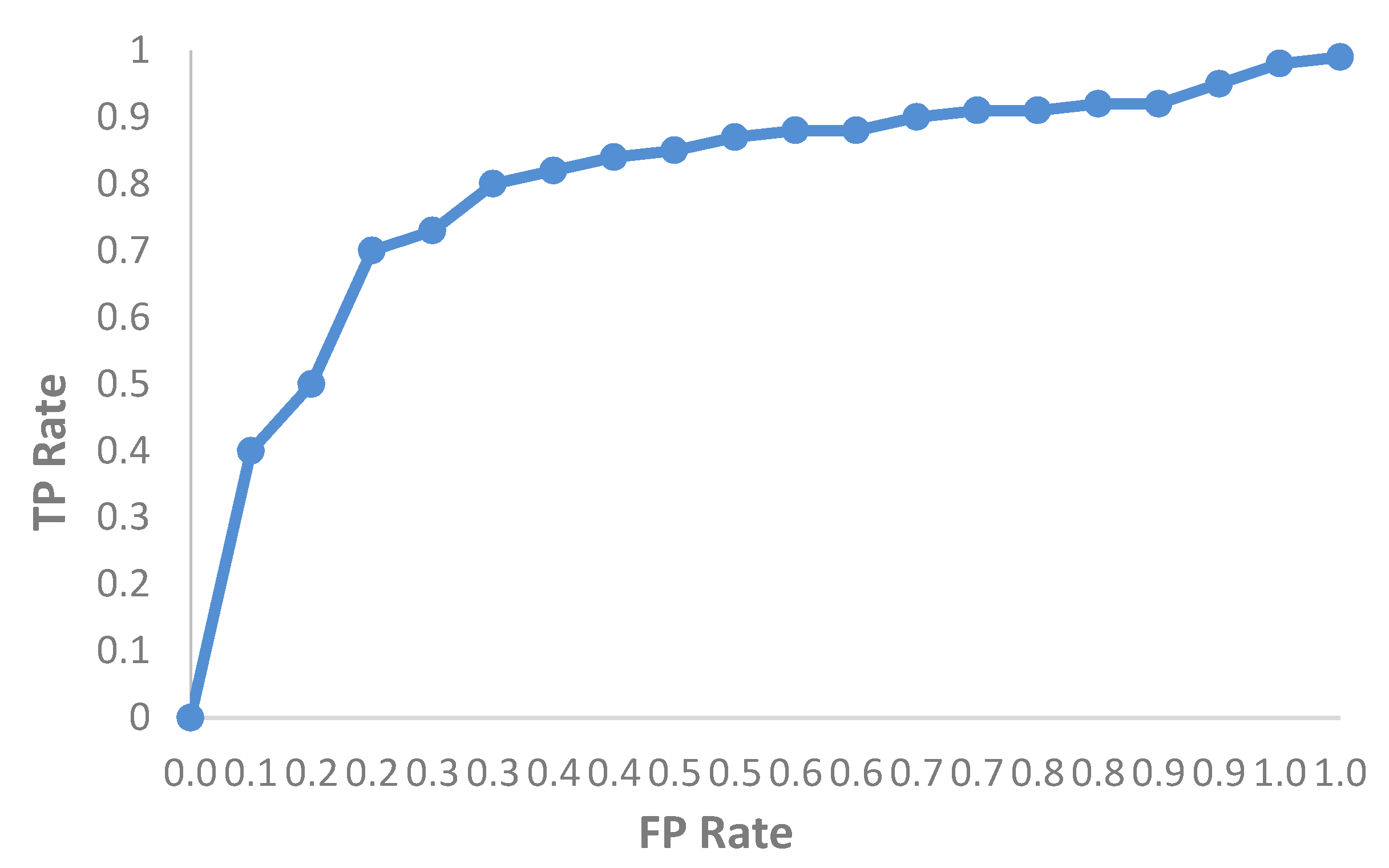
The congestion control dataset was divided into 10% of instances as a test dataset and 90% of all data as a training dataset. The experimental congestion control dataset was comprised of 13% optimal class and 87% non-optimal class. The extraordinary outcome of DT (C4.5) observed from Table 3 shows that C4.5 was the best among the selected algorithms. The optimal TP rate is 1.0, and the TP rate of DT C4.5 was near 0.924—better than both RepTree and random tree. The closer the FP rate is to zero, the more optimal the result. The C4.5 DT FP rate satisfied this condition. Precision and recall values were optimistic because they were close to the optimal value of 1.0. In respect of the extraordinary DT C4.5 performances observed in Table 3, the goal of this research to enhance the network performance by utilizing DT C4.5 was achieved. Additionally, the tree graph of the decision tree allows characterization with simplicity and ease, making it the best choice for analyzing prediction results. Furthermore, ROC was used to clarify the classifier accuracy. Some datasets may achieve a prediction of 92% of instances and result in a non-preferable classifier. The ROC curve can determine whether or not the classifier is appropriate for prediction. The nearer the curve is to 1.0, the better the classifier is. Figure 8 shows that the model was suitable and reliable for prediction. The area under the ROC curve was 0.889, which is a reasonable and optimal value.

4.4. Effect of Delay

Simulations using network topology were conducted to clarify the effect of delay on SCTP congestion control. Delay represents how long it can take for a bit of data to be transmitted across the network from one node to the destination over a specific data link. Delay is presented in multiples or fractions of seconds.

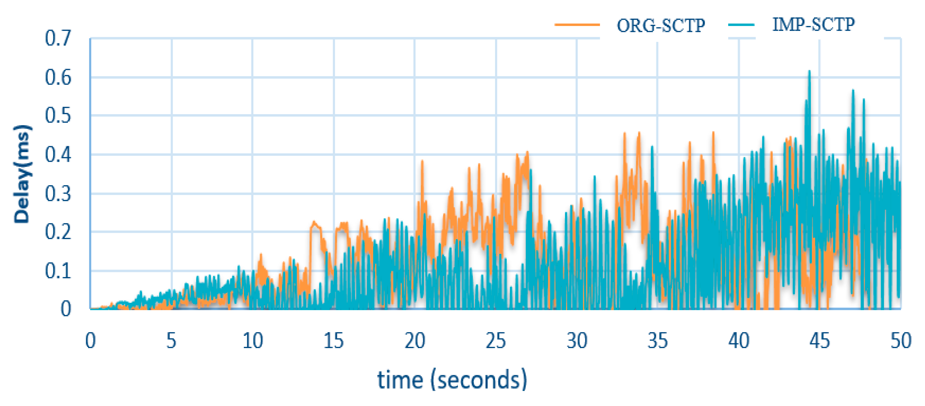
Figure 9 displays the delay up to 50 s. The favorable performance of the proposed congestion control mechanism is clearly reflected in Figure 9. The simulation time was set to 50 s. Given the lack of a congestion control mechanism in ORG-SCTP, the delay was prominent in the high-traffic-load environment. The total delay rates of SCTPs differed significantly within the period of 50 s. The performance of ORG-SCTP deteriorated (high delay indicates poor performance). The proposed congestion control of IMP-SCTP performed 14.5% better than that of ORG-SCTP. The performance of ORG-SCTP showed consistent degradation (Figure 9). ORG-SCTP and IMP-SCTP experienced a slight increase in performance from 1 to 10 s. Beyond 10 s, the delay for ORG-SCTP declined continuously, whereas the delay for IMP-SCTP was less significant. Furthermore, the throughput for ORG-SCTP was minimized from 14 to 26 s and showed the highest drawback at 33–38 s. The delay of ORG-SCTP increased again and continued to fluctuate until the end of the experiment. Thus, IMP-SCTP outperformed ORG-SCTP in terms of delay from 11 to 35 s. IMP-SCTP showed a high delay rate at 45 and 47 s; nevertheless, the delay of IMP-SCTP was less than that of ORG-SCTP. The data in Figure 9 were measured at a time step of 0.05 s. This period was derived from the overall simulation time. Furthermore, the sample was taken from one connection between a specific UE and an eNB across a high-load-traffic bottleneck. The result of the paired sample t-test demonstrates the significant difference between the delays of ORG-SCTP and IMP-SCTP. The mean of the delay for ORG-SCTP (m = 1118.023) was greater than that for IMP-SCTP (m = 971.849). Again, the equation t(df) = t state, p ≤ 0.05, was used to determine the significance of the difference between the two SCTPs, t(1275) = 2.93, p ≤ 0.05. The p-value was 0.003 at 50 s. Given that 0.003 ≤ 0.5, the difference between the delays of ORG-SCTP and IMP-SCTP was significant. Overall, the proposed enhancement improved the delay of IMP-SCTP.

4.5. Effect of Jitter

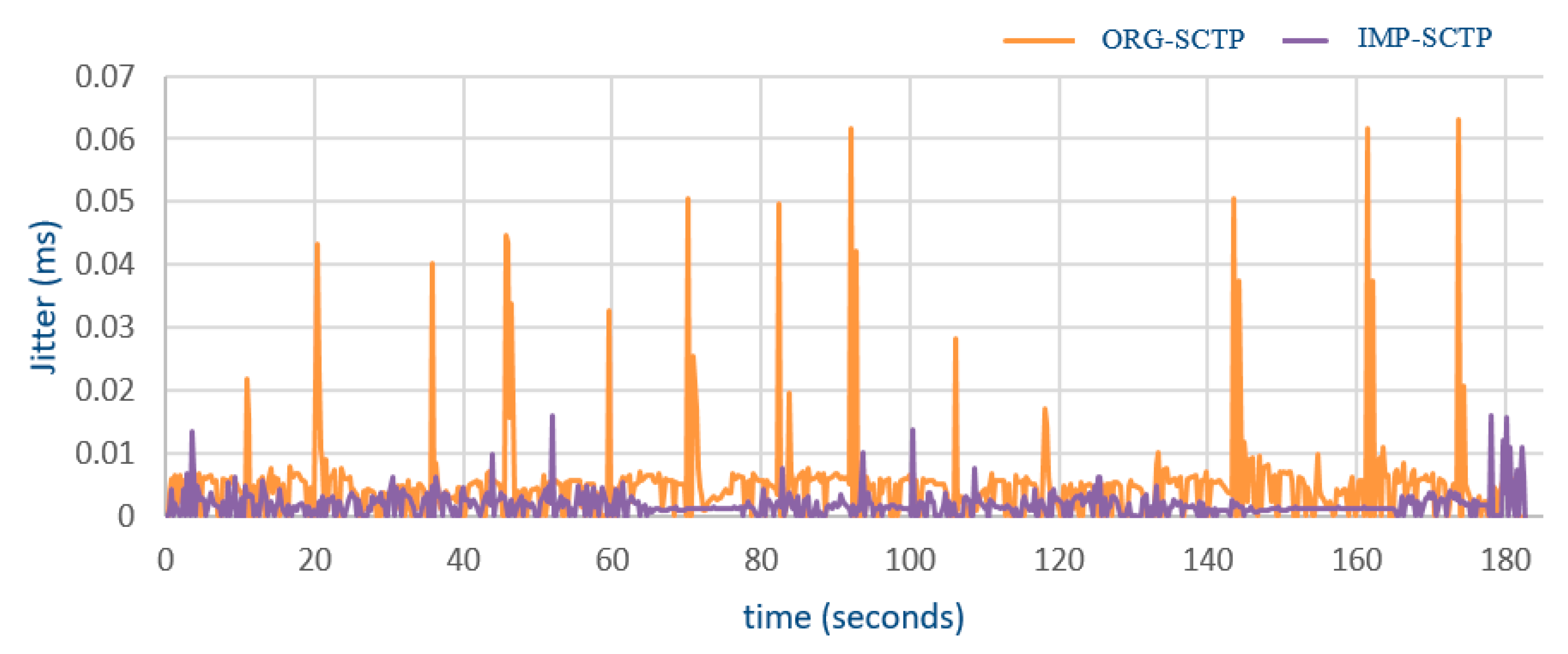
This part shows effect of jitter on the proposed SCTP congestion control. Jitter can be defined as the difference in delay of the received packets. The transmitting side sends packets in a continuous flow and spaces them equally as a variation in the delay of received packets. Due to congestion control, the received packets are either received or dropped. Jitter is used as an impacted utilization to evaluate the performance of the enhanced congestion control mechanism in the post-simulation stage. The average rate of jitter for each flow can represent the router resource management. Figure 10 shows the difference between ORG-SCTP and IMP-SCTP.

This performance parameter was assessed for 180 s. The scale of milliseconds was used as a rate for evaluation. The two SCTPs were started at 0.3 s, and then jitter of ORG-SCTP was maximized from 0.4 to 9 s. It was observed that the performance of IMP-SCTP oscillated slightly but did not reach a higher level than ORG-SCTP. It was observed that although the performance of IMP-SCTP was unstable throughout the simulation period, it was better than that of ORG-SCTP by 64%. Although the performance of IMP-SCTP declined (the rising level in jitter indicates degrading performance), IMP-SCTP was still better than ORG-SCTP. The performance degradations of the latter were evident in the following periods: 13–18 s, 61–69 s, 133–143 s, and 163–172 s. Meanwhile, the lowest performance degradations were observed at 11, 20, 35, 46, 59, 70, 82, 92, 106, 118, 144, 161, 162, and 173 s. Moreover, the jitter utilization of IMP-SCTP increased at 3, 43, 52, 100, 108, and 178–180 s. The performance of IMP-SCTP was better and more stable than that of ORG-SCTP from 10 s to the end of the simulation period, and rarely reached the maximum level. Throughout the 180 s, the behaviors were independent of elapsed time. Since the behaviors were independent of time, the result records are reported in the 180 s. A paired-sample t-test was implemented to calculate the significant difference between jitter levels of IMP-SCTP and ORG-SCTP. The mean of jitter for IMP-SCTP (mean = 0.0017) was less than the mean of ORG-SCTP (mean = 0.005). To determine the significant difference, the equation t(df) = t state (p ≤ 0.05) was used again between two SCTPs, t(703) = 11.65, p ≤ 0.05. The p-values reached 0.0 at 180 s, and since 0.0 ≤ 0.5, the jitter level of IMP-SCTP and ORG-SCTP differed significantly. Therefore, the proposed enhancements improved IMP-SCTP’s jitter.

The improved congestion control based on DT C4.5 machine learning presented superior outcomes to original SCTP in the 5G environment. The new mathematical approaches that were incorporated for the prediction were developed for an improved congestion control approach to acquire the optimal values from the proposed equations. Figure 11 provides the outcomes showing that the throughput, packet loss, cwnd, and queue size were enhanced by 8.5%, 16%, 75%, and 93%, respectively, as compared to conventional SCTP variants. In addition, the jitter was improved, being decreased by 64%, delay was decreased by 14.5%, and the packet send/receive was increased by 20%. It can be concluded that the proposed approach is efficient for wide-bandwidth networks such as 5G IoT.

5. Conclusions

The congestion control problem in all network generations faced by many models necessitates the improvement of network performance through enhanced mechanisms or combinatorial algorithms. This study addressed the congestion control problem in 5G IoT environments by proposing a new model constructed based on a machine learning DT approach to predict the optimal node in 5G IoT environments. The proposed approach can help to improve congestion control and enhance overall network performance. The optimal congestion window management can be determined based on specific conditions, such as high throughput, high queue size, high congestion window, and low packet loss. A table of node readings was adopted to determine the optimal parameter values, and the resulting table was used for the machine learning model to make future predictions of optimal nodes.

The C4.5 DT approach showed superior performance to other ML algorithms; it presents a tree-based graph that helps in finding the optimal alternative and the best path for congestion control. The resulting decision graph is an effective method to make a decision due to its clear presentation of all cases and highly scalable route selection. Many factors, such as low packet loss, high throughput, high queue size, and high congestion window, can affect the determination of optimal nodes in a network. The size of the training dataset can increase the accuracy rate of the results. The larger the training dataset size is, the more accurate the results are. The (C4.5) DT algorithm proved its effectiveness in prediction and classification based on this model. The DT graph can provide a simplified plan to visually determine optimal and non-optimal nodes based on assigned values. Compared with other models that adopt the machine learning approach for improving the performance of congestion control, the proposed model presented promising results, with an accuracy of 92% in terms of predicting the optimal node. The results prove the model’s efficiency and accuracy.

In future work, we will compare three machine learning techniques in congestion control in 5G IoT environments for optimization and enhancement. Further, we will attempt to implement the optimal machine learning prediction techniques on hardware and test it in a real test-bed environment. Machine learning and 5G environments are promising research trends related to the development of prediction and optimization network protocol layers. Other aspects may also be considered for autonomous systems in optimal network utilization improvement, where integration will present a multi-objective domain and obtain multidisciplinary domains like AI and human control and deliver the best network performance.

References

1. Najm, A.; Ismail, M.; Rahem, T.; Al Razak, A. Wireless implementation selection in higher institution learning environment. J. Theor. Appl. Inf. Technol. 2014, 67, 477–484. [Google Scholar]
2. Rahem, A.A.T.; Ismail, M.; Najm, I.A.; Balfaqih, M. Topology sense and graph-based TSG: Efficient wireless ad hoc routing protocol for WANET. Telecommun. Syst. 2017, 65, 739–754. [Google Scholar] [CrossRef]
3. Aalsalem, M.Y.; Khan, W.Z.; Gharibi, W.; Khan, M.K.; Arshad, Q. Wireless Sensor Networks in oil and gas industry: Recent advances, taxonomy, requirements, and open challenges. J. Netw. Comput. Appl. 2018, 113, 87–97. [Google Scholar] [CrossRef]
4. Flora, D.J.; Kavitha, V.; Muthuselvi, M. A survey on congestion control techniques in wireless sensor networks. In Proceedings of the 2011 International Conference Emerging Trends in Electrical and Computer Technology (ICETECT), Nagercoil, India, 23–24 March 2011; pp. 1146–1149. [Google Scholar]
5. Sunny, A.; Panchal, S.; Vidhani, N.; Krishnasamy, S.; Anand, S.; Hegde, M.; Kuri, J.; Kumar, A. A generic controller for managing TCP transfers in IEEE 802.11 infrastructure WLANs. J. Netw. Comput. Appl. 2017, 93, 13–26. [Google Scholar] [CrossRef]
6. Karunakaran, S.; Thangaraj, P. A cluster based congestion control protocol for mobile ad hoc networks. Int. J. Inf. Technol. Knowl. Manag. 2010, 2, 471–474. [Google Scholar]
7. Jain, R. Congestion Control in Computer Networks: Issues and. IEEE Netw. Mag. 1990, 4, 24–30. [Google Scholar] [CrossRef]
8. Kafi, M.A.; Djenouri, D.; Ben-Othman, J.; Badache, N. Congestion control protocols in wireless sensor networks: A survey. IEEE Commun. Surv. Tutor. 2014, 16, 1369–1390. [Google Scholar] [CrossRef]
9. Floyd, S. Congestion Control Principles. 2000. [Google Scholar] [CrossRef]
10. Firoiu, V.; Borden, M. A study of active queue management for congestion control. In Proceedings of the INFOCOM 2000, Nineteenth Annual Joint Conference of the IEEE Computer and Communications Societies, Tel Aviv, Israel, 26–30 March 2000; pp. 1435–1444. [Google Scholar]
11. Qazi, I.A.; Znati, T. On the design of load factor based congestion control protocols for next-generation networks. Comput. Netw. 2011, 55, 45–60. [Google Scholar] [CrossRef] [Green Version]
12. Katabi, D.; Handley, M.; Rohrs, C. Congestion control for high bandwidth-delay product networks. Acm Sigcomm Comput. Commun. Rev. 2002, 32, 89–102. [Google Scholar] [CrossRef]
13. Subramanian, S.; Werner, M.; Liu, S.; Jose, J.; Lupoaie, R.; Wu, X. Congestion control for vehicular safety: Synchronous and asynchronous MAC algorithms. In Proceedings of the ninth ACM International Workshop on Vehicular Inter-Networking, Systems, and Applications, Low Wood Bay, Lake District, UK, 25 June 2012; pp. 63–72. [Google Scholar]
14. Wang, Y.; Rozhnova, N.; Narayanan, A.; Oran, D.; Rhee, I. An improved hop-by-hop interest shaper for congestion control in named data networking. Acm Sigcomm Comput. Commun. Rev. 2013, 43, 55–60. [Google Scholar] [CrossRef] [Green Version]
15. Wischik, D.; Raiciu, C.; Greenhalgh, A.; Handley, M. Design, Implementation and Evaluation of Congestion Control for Multipath TCP. NSDI 2011, 11, 8. [Google Scholar]
16. Mirza, M.; Sommers, J.; Barford, P.; Zhu, X. A machine learning approach to TCP throughput prediction. IEEE/ACM Trans. Netw. (Ton) 2010, 18, 1026–1039. [Google Scholar] [CrossRef]
17. Kong, Y.; Zang, H.; Ma, X. Improving TCP Congestion Control with Machine Intelligence. In Proceedings of the 2018 Workshop on Network Meets AI & ML, Budapest, Hungary, 24 August 2018; pp. 60–66. [Google Scholar]
18. Nunes, B.A.; Veenstra, K.; Ballenthin, W.; Lukin, S.; Obraczka, K. A machine learning approach to end-to-end rtt estimation and its application to tcp. In Proceedings of the 20th International Conference on Computer Communications and Networks (ICCCN), Maui, HI, USA, 31 July–4 August 2011; pp. 1–6. [Google Scholar]
19. Taherkhani, N.; Pierre, S. Centralized and localized data congestion control strategy for vehicular ad hoc networks using a machine learning clustering algorithm. IEEE Trans. Intell. Transp. Syst. 2016, 17, 3275–3285. [Google Scholar] [CrossRef]
20. Fadlullah, Z.; Tang, F.; Mao, B.; Kato, N.; Akashi, O.; Inoue, T.; Mizutani, K. State-of-the-art deep learning: Evolving machine intelligence toward tomorrow’s intelligent network traffic control systems. IEEE Commun. Surv. Tutor. 2017, 19, 2432–2455. [Google Scholar] [CrossRef]
21. González-Landero, F.; García-Magariño, I.; Lacuesta, R.; Lloret, J. PriorityNet App: A mobile application for establishing priorities in the context of 5G ultra-dense networks. IEEE Access 2018, 6. [Google Scholar] [CrossRef]
22. Lloret, J.; Parra, L.; Taha, M.; Tomas, J. An architecture and protocol for smart continuous eHealth monitoring using 5G. Comput. Netw. 2017, 129, 340–351. [Google Scholar] [CrossRef]
23. Taha, M.; Parra, L.; Garcia, L.; Lloret, J. An Intelligent handover process algorithm in 5G networks: The use case of mobile cameras for environmental surveillance. In Proceedings of the 2017 IEEE International Conference on Communications Workshops (ICC Workshops), Paris, France, 21–25 May 2017; pp. 840–844. [Google Scholar]
24. Khan, I.; Zafar, M.H.; Jan, M.T.; Lloret, J.; Basheri, M.; Singh, D. Spectral and Energy Efficient Low-Overhead Uplink and Downlink Channel Estimation for 5G Massive MIMO Systems. Entropy 2018, 20, 92. [Google Scholar] [CrossRef]
25. Sangeetha, G.; Vijayalakshmi, M.; Ganapathy, S.; Kannan, A. A Heuristic Path Search for Congestion Control in WSN. Ind. Int. Innov. Sci. Eng. Technol. 2018, 11, 485–495. [Google Scholar]
26. Elappila, M.; Chinara, S.; Parhi, D.R. Survivable path routing in WSN for IoT applications. Pervasive Mob. Comput. 2018, 43, 49–63. [Google Scholar] [CrossRef]
27. Singh, K.; Singh, K.; Aziz, A. Congestion control in wireless sensor networks by hybrid multi-objective optimization algorithm. Comput. Netw. 2018, 138, 90–107. [Google Scholar] [CrossRef]
28. Shelke, M.; Malhotra, A.; Mahalle, P.N. Congestion-Aware Opportunistic Routing Protocol in Wireless Sensor Networks. Smart Comput. Inf. 2018, 77, 63–72. [Google Scholar]
29. Godoy, P.D.; Cayssials, R.L.; Garino, C.G.G. Communication channel occupation and congestion in wireless sensor networks. Comput. Electr. Eng. 2018, 72, 846–858. [Google Scholar] [CrossRef]
30. Najm, I.A.; Ismail, M.; Lloret, J.; Ghafoor, K.Z.; Zaidan, B.; Rahem, A.A.R.T. Improvement of SCTP congestion control in the LTE-A network. J. Netw. Comput. Appl. 2015, 58, 119–129. [Google Scholar] [CrossRef]
31. Najm, I.A.; Ismail, M.; Abed, G.A. High-performance mobile technology LTE-A using the stream control transmission protocol: A systematic review and hands-on analysis. J. Appl. Sci. 2014, 14, 2194–2218. [Google Scholar] [CrossRef]
32. Geurts, P.; El Khayat, I.; Leduc, G. A machine learning approach to improve congestion control over wireless computer networks. In Proceedings of the Fourth IEEE International Conference on Data Mining (ICDM’04), Brighton, UK, 1–4 November 2004; pp. 383–386. [Google Scholar]
33. Brahma, S.; Chatterjee, M.; Kwiat, K. Congestion control and fairness in wireless sensor networks. In Proceedings of the 8th IEEE International Conference on Pervasive Computing and Communications Workshops (PERCOM Workshops), Mannheim, Germany, 29 March–2 April 2010; pp. 413–418. [Google Scholar]
34. Jagannathan, S.; Almeroth, K.C. Using tree topology for multicast congestion control. In Proceedings of the International Conference on Parallel Processing, Valencia, Spain, 3–7 September 2001; p. 313. [Google Scholar]
35. Katuwal, R.; Suganthan, P.; Zhang, L. An ensemble of decision trees with random vector functional link networks for multi-class classification. Appl. Soft Comput. 2018, 70, 1146–1153. [Google Scholar] [CrossRef]
36. Gómez, S.E.; Martínez, B.C.; Sánchez-Esguevillas, A.J.; Callejo, L.H. Ensemble network traffic classification: Algorithm comparison and novel ensemble scheme proposal. Comput. Netw. 2017, 127, 68–80. [Google Scholar] [CrossRef]
37. Hasan, M.; Hossain, E.; Niyato, D. Random access for machine-to-machine communication in LTE-advanced networks: Issues and approaches. IEEE Commun. Mag. 2013, 51, 86–93. [Google Scholar] [CrossRef]
38. Leng, B.; Huang, L.; Qiao, C.; Xu, H. A decision-tree-based on-line flow table compressing method in software defined networks. In Proceedings of the 2016 IEEE/ACM 24th International Symposium on Quality of Service (IWQoS), Beijing, China, 20–21 June 2016; pp. 1–2. [Google Scholar]
39. Liang, D.; Zhang, Z.; Peng, M. Access Point Reselection and Adaptive Cluster Splitting-Based Indoor Localization in Wireless Local Area Networks. IEEE Internet Things. J. 2015, 2, 573–585. [Google Scholar] [CrossRef]
40. Liu, Y.; Wu, H. Prediction of Road Traffic Congestion Based on Random Forest. In Proceedings of the 2017 10th International Symposium on Computational Intelligence and Design (ISCID), Hangzhou, China, 9–10 December 2017; pp. 361–364. [Google Scholar]
41. Park, H.; Haghani, A.; Samuel, S.; Knodler, M.A. Real-time prediction and avoidance of secondary crashes under unexpected traffic congestion. Accid. Anal. Prev. 2018, 112, 39–49. [Google Scholar] [CrossRef]
42. Shu, J.; Liu, S.; Liu, L.; Zhan, L.; Hu, G. Research on link quality estimation mechanism for wireless sensor networks based on support vector machine. Chin. J. Electron. 2017, 26, 377–384. [Google Scholar] [CrossRef]
43. Riekstin, A.C.; Januário, G.C.; Rodrigues, B.B.; Nascimento, V.T.; Carvalho, T.C.; Meirosu, C. Orchestration of energy efficiency capabilities in networks. J. Netw. Comput. Appl. 2016, 59, 74–87. [Google Scholar] [CrossRef]
44. Soltani, S.; Mutka, M.W. Decision tree modeling for video routing in cognitive radio mesh networks. In Proceedings of the IEEE 14th International Symposium on “A World of Wireless, Mobile and Multimedia Networks” (WoWMoM), Madrid, Spain, 4–7 June 2013; pp. 1–9. [Google Scholar]
45. Adi, E.; Baig, Z.; Hingston, P. Stealthy Denial of Service (DoS) attack modelling and detection for HTTP/2 services. J. Netw. Comput. Appl. 2017, 91, 1–13. [Google Scholar] [CrossRef]
46. Stimpfling, T.; Bélanger, N.; Cherkaoui, O.; Béliveau, A.; Béliveau, L.; Savaria, Y. Extensions to decision-tree based packet classification algorithms to address new classification paradigms. Comput. Netw. 2017, 122, 83–95. [Google Scholar] [CrossRef]
47. Singh, D.; Nigam, S.; Agrawal, V.; Kumar, M. Vehicular traffic noise prediction using soft computing approach. J. Environ. Manag. 2016, 183, 59–66. [Google Scholar] [CrossRef]
48. Xia, Y.; Chen, W.; Liu, X.; Zhang, L.; Li, X.; Xiang, Y. Adaptive multimedia data forwarding for privacy preservation in vehicular ad-hoc networks. IEEE Trans. Intell. Transp. Syst. 2017, 18, 2629–2641. [Google Scholar] [CrossRef]
49. Tariq, F.; Baig, S. Machine Learning Based Botnet Detection in Software Defined Networks. Int. J. Secur. Appl. 2017, 11, 1–11. [Google Scholar] [CrossRef]
50. Wu, T.; Petrangeli, S.; Huysegems, R.; Bostoen, T.; De Turck, F. Network-based video freeze detection and prediction in HTTP adaptive streaming. Comput. Commun. 2017, 99, 37–47. [Google Scholar] [CrossRef]
51. Chen, Y.-y.; Lv, Y.; Li, Z.; Wang, F.-Y. Long short-term memory model for traffic congestion prediction with online open data. In Proceedings of the 2016 IEEE 19th International Conference Intelligent Transportation Systems (ITSC), Rio de Janeiro, Brazil, 1–4 November 2016; pp. 132–137. [Google Scholar]
52. Abar, T.; Letaifa, A.B.; El Asmi, S. Machine learning based QoE prediction in SDN networks. In Proceedings of the 13th International Wireless Communications and Mobile Computing Conference (IWCMC), Valencia, Spain, 26–30 June 2017; pp. 1395–1400. [Google Scholar]
53. Pham, T.N.D.; Yeo, C.K. Adaptive trust and privacy management framework for vehicular networks. Veh. Commun. 2018, 13, 1–12. [Google Scholar] [CrossRef]
54. Mohamed, M.F.; Shabayek, A.E.-R.; El-Gayyar, M.; Nassar, H. An adaptive framework for real-time data reduction in AMI. J. King Saud Univ. Comput. Inf. Sci. 2018. [Google Scholar] [CrossRef]
55. Tierney, B.; Kissel, E.; Swany, M.; Pouyoul, E. Efficient data transfer protocols for big data. In Proceedings of the IEEE 8th International Conference on E-Science, Chicago, IL, USA, 8–12 October 2012; pp. 1–9. [Google Scholar]
56. Brennan, R.; Curran, T. SCTP congestion control: Initial simulation studies. In Proceedings of the International Teletraffic Congress (ITC 17), Salvador da Bahia, Brazil, 2–7 December 2001. [Google Scholar]
57. Louvieris, P.; Clewley, N.; Liu, X. Effects-based feature identification for network intrusion detection. Neurocomputing 2013, 121, 265–273. [Google Scholar] [CrossRef]
58. Chen, J. Congestion control mechanisms of transport protocols. In Proceedings of the ACM/IEEE Conference on Supercomputing, New York, NY, USA, 8–12 June 2009. [Google Scholar]
59. Ahmed, I.; Yasuo, O.; Masanori, K. Improving performance of SCTP over broadband high latency networks. In Proceedings of the 28th Annual IEEE International Conference on Local Computer Networks, 2003, LCN’03, Bonn/Konigswinter, Germany, 20–24 October 2003; pp. 644–645. [Google Scholar]
60. Ye, G.; Saadawi, T.; Lee, M. SCTP congestion control performance in wireless multi-hop networks. In Proceedings of the MILCOM 2002, Proceedings, Anaheim, CA, USA, 7–10 October 2002; pp. 934–939. [Google Scholar]
61. Witten, I.H.; Frank, E.; Hall, M.A.; Pal, C.J. Data Mining: Practical Machine Learning Tools and Techniques; Morgan Kaufmann: Cambridge, MA, USA, 2016. [Google Scholar]
62. HAMOUD, A.K. Classifying Students’ Answers Using Clustering Algorithms Based on Principle Component Analysis. J. Theor. Appl. Infor. Technol. 2018, 96, 1813–1825. [Google Scholar]
63. Verma, P.K.; Verma, R.; Prakash, A.; Agrawal, A.; Naik, K.; Tripathi, R.; Alsabaan, M.; Khalifa, T.; Abdelkader, T.; Abogharaf, A. Machine-to-Machine (M2M) communications: A survey. J. Netw. Comput. Appl. 2016, 66, 83–105. [Google Scholar] [CrossRef]
64. Ibrahim, Z.; Rusli, D. Predicting students’ academic performance: Comparing artificial neural network, decision tree and linear regression. In Proceedings of the 21st Annual SAS Malaysia Forum, Shangri-La Hotel, Kuala Lumpur, Malaysia, 5 September 2007; pp. 1–6. [Google Scholar]
65. Hamoud, A.K. Selection of Best Decision Tree Algorithm for Prediction and Classification of Students’ Action. Am. Int. J. Res. Sci. Technol. Eng. Math. 2016, 16, 26–32. [Google Scholar]
66. Hamoud, A.K.; Hashim, A.S.; Awadh, W.A. Predicting Student Performance in Higher Education Institutions Using Decision Tree Analysis. Int. J. Interact. Multimed. Artif. Intell. 2018, 5, 26–31. [Google Scholar] [CrossRef]
67. Hamoud, A.K. Applying Association Rules and Decision Tree Algorithms with Tumor Diagnosis Data. Int. Res. J. Eng. Technol. 2017, 3, 27–31. [Google Scholar]
68. Lavanya, D.; Rani, K.U. Ensemble decision tree classifier for breast cancer data. Int. J. Inf. Technol. Converg. Serv. 2012, 2, 17. [Google Scholar] [CrossRef]
69. Polat, K.; Güneş, S. Classification of epileptiform EEG using a hybrid system based on decision tree classifier and fast Fourier transform. Appl. Math. Comput. 2007, 187, 1017–1026. [Google Scholar] [CrossRef]
70. Rajput, A.; Aharwal, R.P.; Dubey, M.; Saxena, S.; Raghuvanshi, M. J48 and JRIP rules for e-governance data. Int. J. Comput. Sci. Secur. (Ijcss) 2011, 5, 201. [Google Scholar]
71. Cayirci, E.; Tezcan, H.; Dogan, Y.; Coskun, V. Wireless sensor networks for underwater survelliance systems. Ad Hoc Netw. 2006, 4, 431–446. [Google Scholar] [CrossRef]
72. Feng, T.; Liu, Z.; Kwon, K.-A.; Shi, W.; Carbunar, B.; Jiang, Y.; Nguyen, N. Continuous mobile authentication using touchscreen gestures. In Proceedings of the 2012 IEEE Conference on Technologies for Homeland Security (HST), Waltham, MA, USA, 13–15 November 2012; pp. 451–456. [Google Scholar]
73. Stein, G.; Chen, B.; Wu, A.S.; Hua, K.A. Decision tree classifier for network intrusion detection with GA-based feature selection. In Proceedings of the 43rd annual Southeast regional conference, Kennesaw, Georgia, 18–20 March 2005; pp. 136–141. [Google Scholar]
74. Sahu, S.; Mehtre, B.M. Network intrusion detection system using J48 Decision Tree. In Proceedings of the 2015 International Conference on Advances in Computing, Communications and Informatics (ICACCI), Kochi, India, 10–13 August 2015; pp. 2023–2026. [Google Scholar]
75. Wilkinson, L. Classification and regression trees. Systat 2004, 11, 35–56. [Google Scholar]
76. Bhargava, N.; Sharma, G.; Bhargava, R.; Mathuria, M. Decision tree analysis on j48 algorithm for data mining. Int. J. Adv. Res. Comput. Sci. Softw. Eng. 2013, 3, 1114–1119. [Google Scholar]
77. Korting, T.S. C4. 5 Algorithm and Multivariate Decision Trees. Image Processing Division, National Institute for Space Research; INPE: Sao Jose dos Campos, SP, Brazil, 2006. [Google Scholar]
78. Hamoud, A.; Humadi, A.; Awadh, W.A.; Hashim, A.S. Students’ Success Prediction based on Bayes Algorithms. Int. J. Comput. Appl. 2017, 178, 6–12. [Google Scholar]
79. Mezzavilla, M.; Zhang, M.; Polese, M.; Ford, R.; Dutta, S.; Rangan, S.; Zorzi, M. End-to-end simulation of 5g mmwave networks. IEEE Commun. Surv. Tutor. 2018, 20, 2237–2263. [Google Scholar] [CrossRef]
80. Rebato, M.; Polese, M.; Zorzi, M. Multi-Sector and Multi-Panel Performance in 5G mmWave Cellular Networks. In Proceedings of the 2018 IEEE Global Communications Conference (GLOBECOM), Abu Dhabi, United Arab Emirates, 9–13 December 2018. [Google Scholar]
Figure 1. Understanding of the development phase. DT: decision tree.
Electronics 08 00607 g001
Figure 2. Flowchart of the proposed congestion control mechanism. ACKed: acknowledgement; ORG-SCTP: original stream control transmission protocol.
Electronics 08 00607 g002
Figure 3. DT visualization.
Electronics 08 00607 g003
Figure 4. Simulation setup. mmWave: millimeter wave; PGW: core gateway; SCTP: stream control transmission protocol; TCP: transmission control protocol.
Electronics 08 00607 g004
Figure 5. Determination of optimal alternatives.
Electronics 08 00607 g005
Figure 6. Congestion control DT.
Electronics 08 00607 g006
Figure 7. Prediction margin of optimal alternatives. AA: actual alternative; PA: predicted alternative.
Electronics 08 00607 g007
Figure 8. Receiver operating characteristic (ROC) curve for the C4.5 DT classifier.
Electronics 08 00607 g008
Figure 9. Delay of ORG-SCTP and improved SCTP (IMP-SCTP).
Electronics 08 00607 g009
Figure 10. Jitter of ORG-SCTP and IMP-SCTP.
Electronics 08 00607 g010
Figure 11. ORG-SCTP versus IMP-SCTP.
Electronics 08 00607 g011