Photovoltaic Module Array Global Maximum Power Tracking Combined with Artificial Bee Colony and Particle Swarm Optimization Algorithm

Abstract

In this study, the output characteristics of partial modules in a photovoltaic module array when subject to shading were first explored. Then, an improved particle swarm optimization (PSO) algorithm was applied to track the global maximum power point (MPP), with a multi-peak characteristic curve. The improved particle swarm optimization algorithm proposed, combined with the artificial bee colony (ABC) algorithm, was used to adjust the weighting, cognition learning factor, and social learning factor, and change the number of iterations to enhance the tracking performance of the MPP tracker. Finally, MATLAB software was used to carry out a simulation and prove the improved that the PSO algorithm successfully tracked the MPP in the photovoltaic array output curve with multiple peaks. Its tracking performance is far superior to the existing PSO algorithm.

1. Introduction

Since the output power of the photovoltaic module array is influenced by external factors such as the current amount of sunlight, ambient temperature, and stains, the output power presents a non-linear change. Therefore, a maximum power tracker must be used to control the output power and maintain it at the maximum power point (MPP). At present, the more commonly used maximum power tracking methods include voltage feedback [1], constant voltage [2], power feedback [3], perturb and observe (P&O) [4], incremental conductance (INC) [5], etc. Among them, voltage feedback is suitable for relatively stable regions. Firstly, the voltage size of the MPP of the photovoltaic module array under specific sunlight intensity and temperature is measured. Then, by adjusting the terminal voltage of the photovoltaic module array to the same voltage as the previously measured MPP, maximum power tracking can be achieved [1]. One advantage of this method is that it facilitates simple judgment; however, a disadvantage is that, when the atmospheric conditions substantially change, the new MPP cannot be instantly tracked. On the other hand, the constant voltage tracking method [2] uses the MPP of the characteristic curve of respective output powers and voltages, which generally corresponds to a constant voltage and then achieves maximum power tracking. It also has the advantage of simple control without complicated calculations, but its disadvantage is that, when the atmospheric environment substantially changes, the new MPP cannot be tracked. Power feedback [3] on the other hand uses the output power and voltage change ratio dP/dV of the photovoltaic module array for logical judgement. This method can reduce energy loss and enhance overall efficiency. The disadvantage is that the sensing component in the actual circuit cannot achieve a precise measurement, and the likelihood of the system operating at the power and voltage curve gradient of zero is extremely low. As for P&O [4], fixed cycles are used to increase or decrease the terminal voltage of the photovoltaic module array. If the voltage perturbance increases the output power of the photovoltaic module array, perturbance in the same direction is performed the next time; if not, perturbance in the opposite direction is performed. The advantage is that the architecture is simple, and only a few measurement parameters are needed, but the disadvantage is that the MPP cannot be precisely tracked, resulting in oscillation occurrence near the maximum power output point and increased tracking loss. The incremental conductance method [5] uses the power–voltage gradient when the photovoltaic module array is at the MPP as the judgement basis. It has the advantages of precise control and fast responses, but it also has drawbacks, such as a large amount of calculation and high controller costs. The existing maximum power tracking methods above are not applicable for photovoltaic module arrays with partial module shading or malfunctioning work conditions. In a photovoltaic module array with partial shading or malfunction, the non-linear output characteristic curve features multiple peaks [6]. Hence, if the traditional maximum power tracking methods are adopted, it is unlikely to skip a local solution to find the actual global optimum solution.

In recent years, many scholars engaged in studies targeting the maximum power tracking method when the multi-peak phenomenon occurs due to the shading of partial models in the module array. The most common smart metaheuristic algorithms at present include fuzzy control (FC) [7], genetic algorithm (GA) [8], neural network (NN) [9], and artificial bee colony (ABC) algorithms [10]. However, as far as FC and NN are concerned, the control process is complex with a large amount of calculation; thus, the actualization difficulty. As for GA and ABC, their applications are limited to the maximum power tracking of a photovoltaic module array with a single-peak value output characteristic curve or without module shading [11]. Compared to traditional maximum power tracking methods, it has a higher success rate in searching global MPPs.

Although the geometric algorithm of the Lipschitz optimization method [12] can accurately track to the global optimal value, it needs complex calculations and it needs to set a lot of parameters. The global optimization technique based on an iterative adaptive efficient partition algorithm (EPA) [13] was proposed to demonstrate that it can obtain the optimal solution in a significantly fewer number of function trials than a conventional GA. However, its calculation is just as complex, and it also needs more parameters; it even needs a preliminary understanding of and experience with the system. In the past, when we solved the optimization problem, deterministic techniques based on the mathematical programming method were often used; however, with the increase of the demand in the real world, it was no longer possible to only use the mathematical programming method to find the optimal solution. Instead, the metaheuristic techniques are used to shorten the calculation time for solving the optimization problem. Although the deterministic optimization algorithm proposed in References [14,15] has a smaller number of iterations than the traditional PSO and ABC methods, it is more complex in design and not easy to implement. Furthermore, for the traditional PSO and ABC optimization methods, their parameters are fixed; thus, the number of iterations will be greater.

In view of the above maximum power tracking methods, maximum power tracking can only be applied in photovoltaic module arrays with a single-peak value output characteristic curve. This paper implements the ABC, with improvements made to successfully skip the local MPP when the module is subject to different shading ratios, producing a P–V characteristic curve with two-peak, three-peak, and four-peak values, thereby quickly and stably tracking the global MPP. This paper uses the ABC optimization method to adjust the parameters of the traditional PSO. In this way, the number of iterations can be reduced and then the time of the maximum power point tracking can be shortened. Moreover, the combined method of PSO and ABC can reduce the standard deviations of the needed number of iterations and even exceed the deterministic techniques.

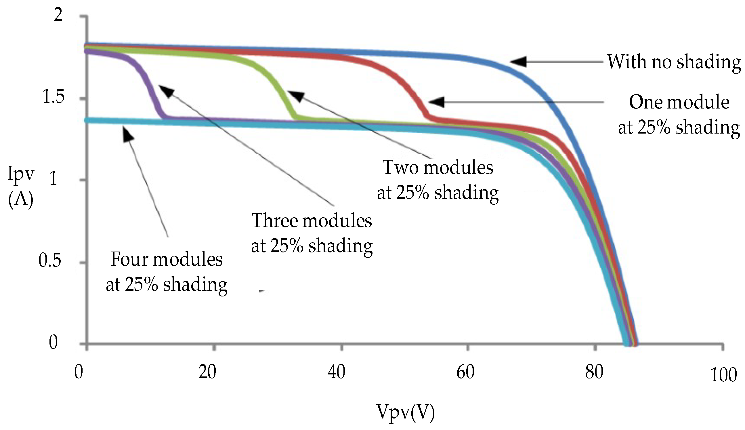
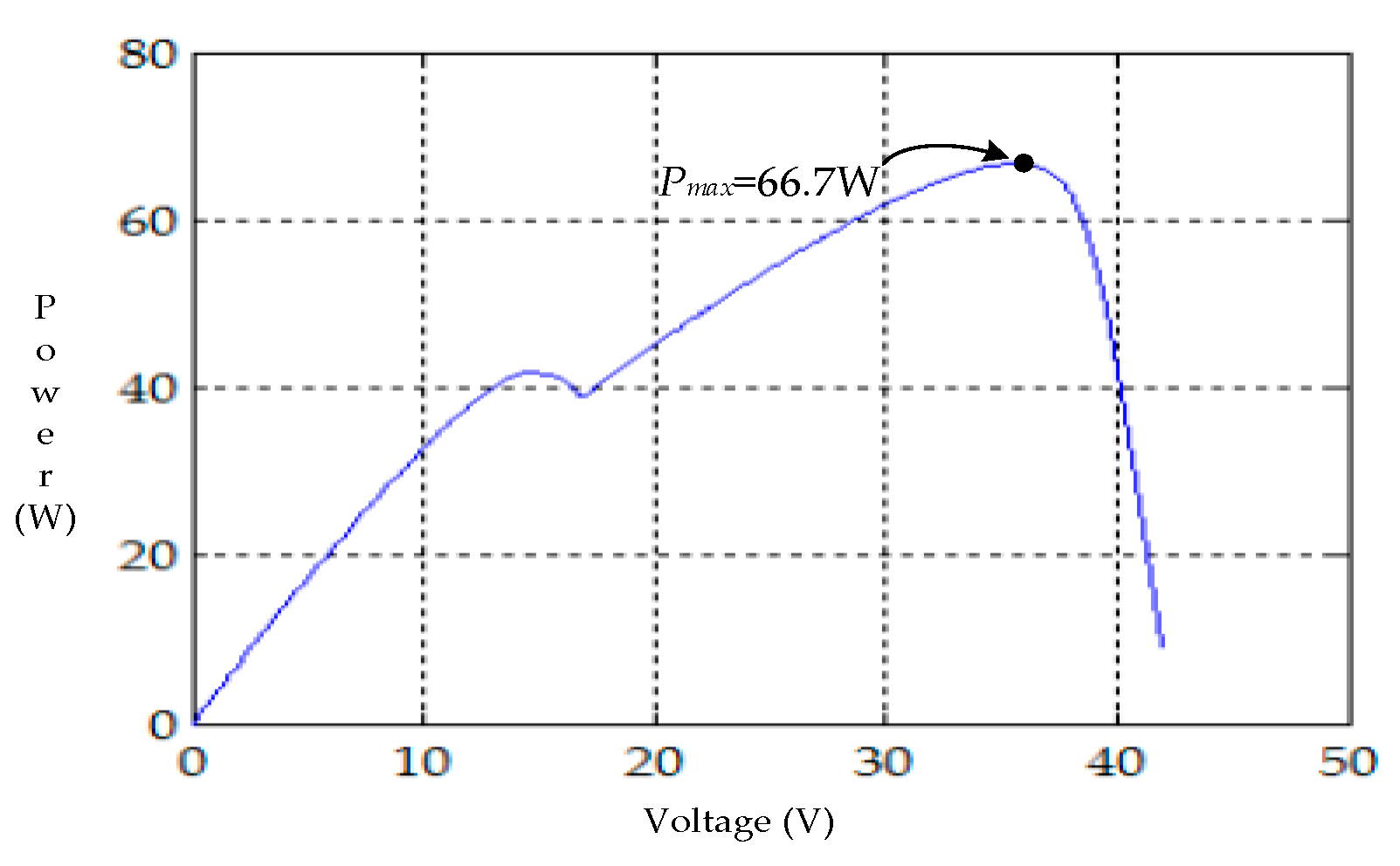
2. The Characteristics of a Photovoltaic Module Array

In a photovoltaic power generation system, in order to obtain a larger output power, photovoltaic modules are usually connected in series or parallel into a module array. However, when the photovoltaic module array is shaded by external factors, such as clouds, trees, buildings, or stains, the output power curve shows non-linear changes and multi-peak values.

In order to explore the output characteristics of photovoltaic module arrays when partial modules connected in series and parallel are shaded, this paper used the HIP2717 module manufactured by SANYO as the research target, which forms a photovoltaic module array connected in four series and one parallel. Figure 1 and Figure 2 show the use of Solar Pro software [16] to simulate the I–V output characteristic curve and P–V output characteristic curve when the one-module, two-module, three-module, and four-module shading ratio was 25% in the module array. An observation of the figures shows that, when partial modules in the array are shaded, not only are multi-peak values produced in the output characteristic curves, but the maximum output power point also has a greater extent of decrease as the number of shaded modules increases.

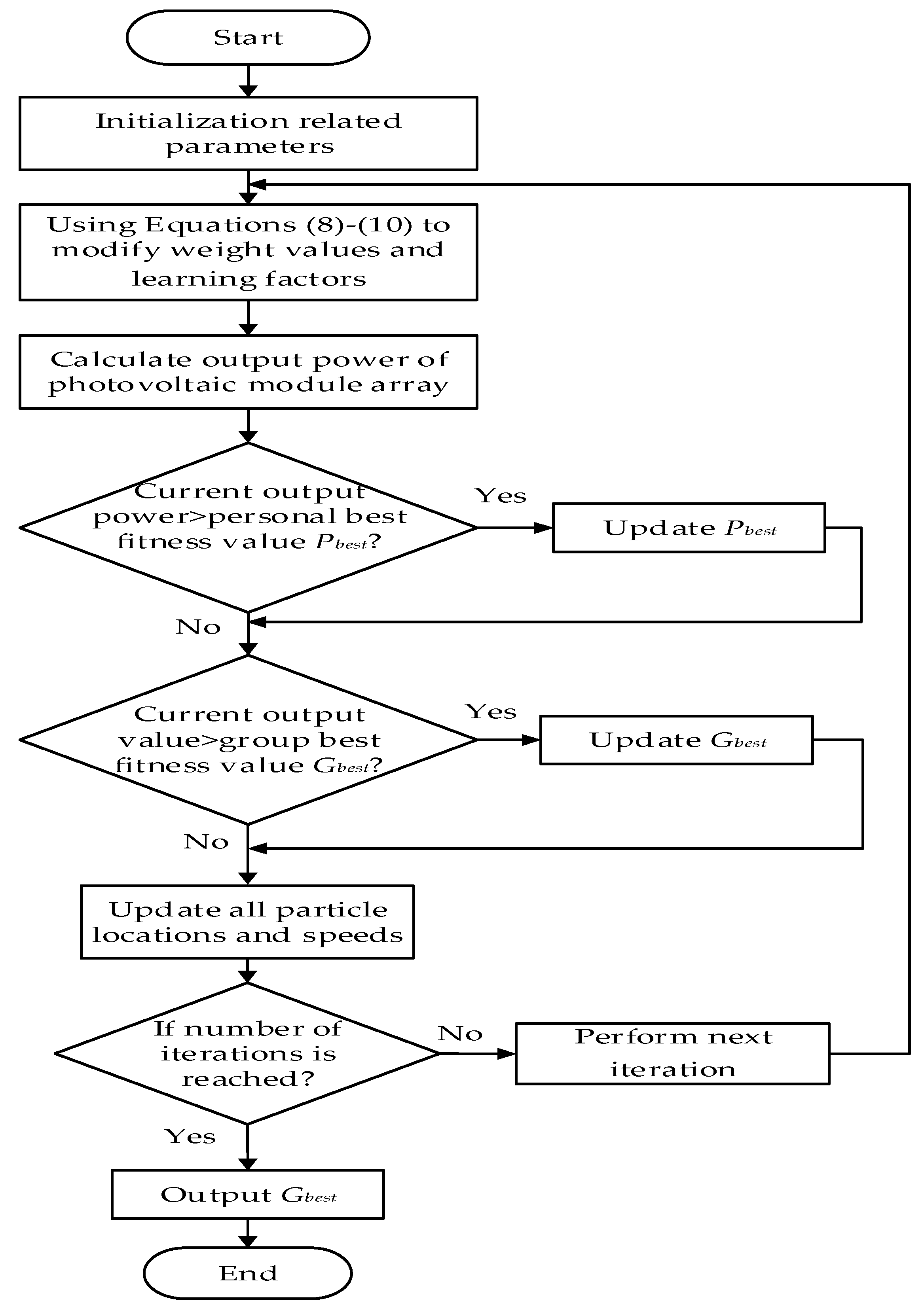
3. Particle Swarm Optimization Algorithm

Particle swarm optimization (PSO) is a type of artificial intelligence (AI)-based algorithm proposed by Eberhart and Kennedy in 1995 [17], who were inspired by observing messages transmitted among birds in search of food. The algorithm is applied in solving search- and optimization-related problems [18,19]. Each bird flying in the space is called a particle, and all the particles moving in the space have a fitness value mapped by the objective function. Each particle has its own velocity, which determines the direction and distance from which each of the particles moves. Particles moving in the space are influenced by two memory values, and each particle stores the current best location found in the best memory location in the individual. At the same time, the memory intercommunication feature exists among the particles, and the particle swarm compares the best location and stores it in the best location in the group. The particle swarm continues to correct the moving direction and speed through this model, thereby rapidly converging to the global optimum solution.

3.1. Traditional Particle Swarm Optimization Algorithm

The flow of the traditional PSO algorithm is as follows:

• Set the number of particles, the maximum number of iterations, weight values, and learning factors.
• Initialize the particle swarm, and randomly set the location and speed of each particle.
• Substitute the initialization location into the objective function to evaluate the fitness function value of the particles.
• The fitness function values of each particle are compared to each other to select a best value $P_{best,j}$. If this best value is larger than the one $(P_{best,j-1})$ we got in the previous iteration, it will be used to replace the optimal value obtained the last time.
• $P_{best}$ and the swarm’s best memory value are compared. If $P_{best}$ is superior to $G_{best}$, it is updated.
• The core formula of the PSO is used to update the particle speed and location. The formula is as shown in Equations (1) and (2).

  $$V_i^{j+1}=W\times V_i^j+C_1\times rand1(·)\times (P_{best,i}-P_i^j)+C_2\times rand2(·)\times ({\mathit{G}}_{\mathit{best}}-P_{\mathit{i}}^j).$$

  (1)

  $$P_i^{j+1}=V_i^{j+1}+P_i^j.$$

  (2)
• If the termination conditions are met, tracking stops; otherwise, repeat Step 4 through Step 6, and the termination condition is to reach the highest number of iterations.

The relevant parameters used in the traditional PSO are described below.

• Weight value (W): Represents the correlation with the last moving distance of its own particles.
• Cognition learning factor (C₁): Represents the learning parameters related to its own particles.
• Social learning factor (C₂): Represents the learning parameters related to other particles.
• $V_i^j$: Represents the moving speed of i number of particles at j number of iterations.
• $P_i^j$: Represents the location of i number of particles at j number of iterations.
• rand1($•$): Represents the first set of random number generator, which produces values between 0 and 1.
• rand2($•$): Represents the second set of random number generator, which produces values between 0 and 1.
• $P_{best,i}$: Represents the personal best solution of i number of particles.
• $G_{best}$: Represents the best solution of the group.

The weight value and learning factor setting value in PSO influence the success rate and tracking efficiency [20]. When the weight value is too small, the particle is too small when moving, resulting in a multi-peak problem, and failing to precisely skip the local best solution; on the contrary, when the weight value setting is too large, the particle is too large when moving, resulting in failure to precisely search the target function. Thus, the selection of a weight value usually depends on the target function. In addition, if the learning factor setting is too large, the iteration time spent increases, resulting in reduced overall tracking efficiency. Therefore, in consideration of the benefits, C₁ and C₂ values set must not be too large.

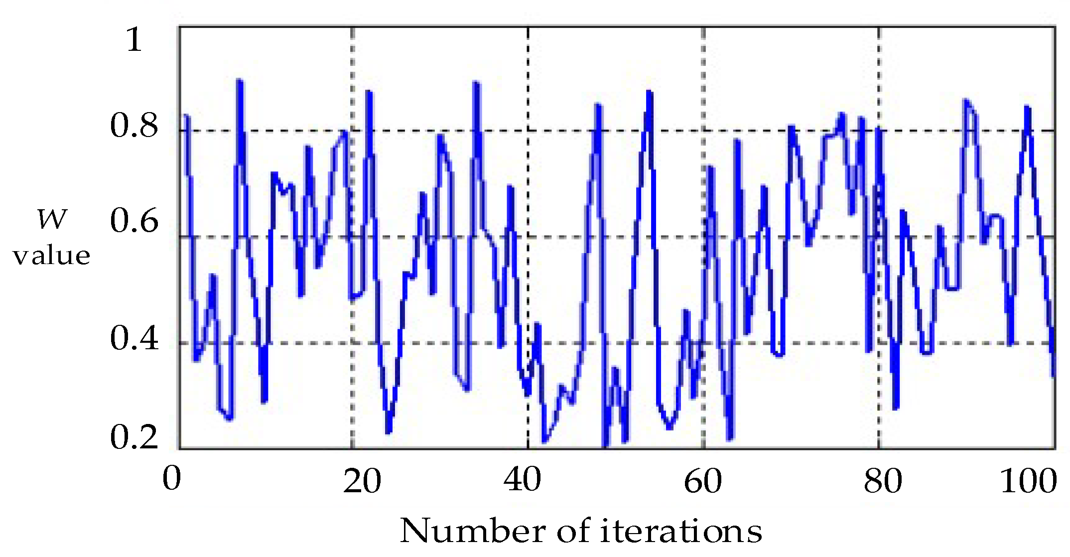
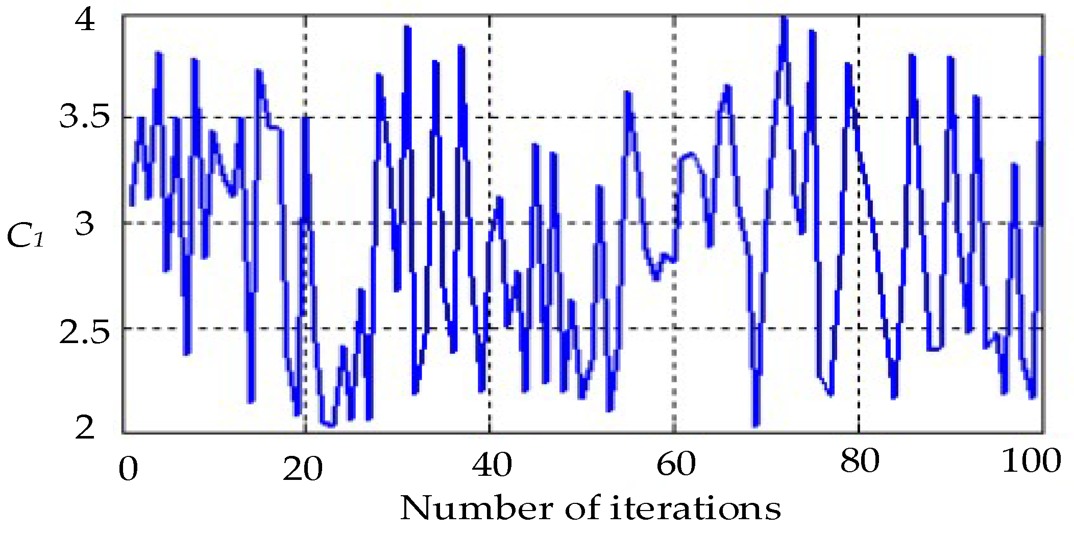
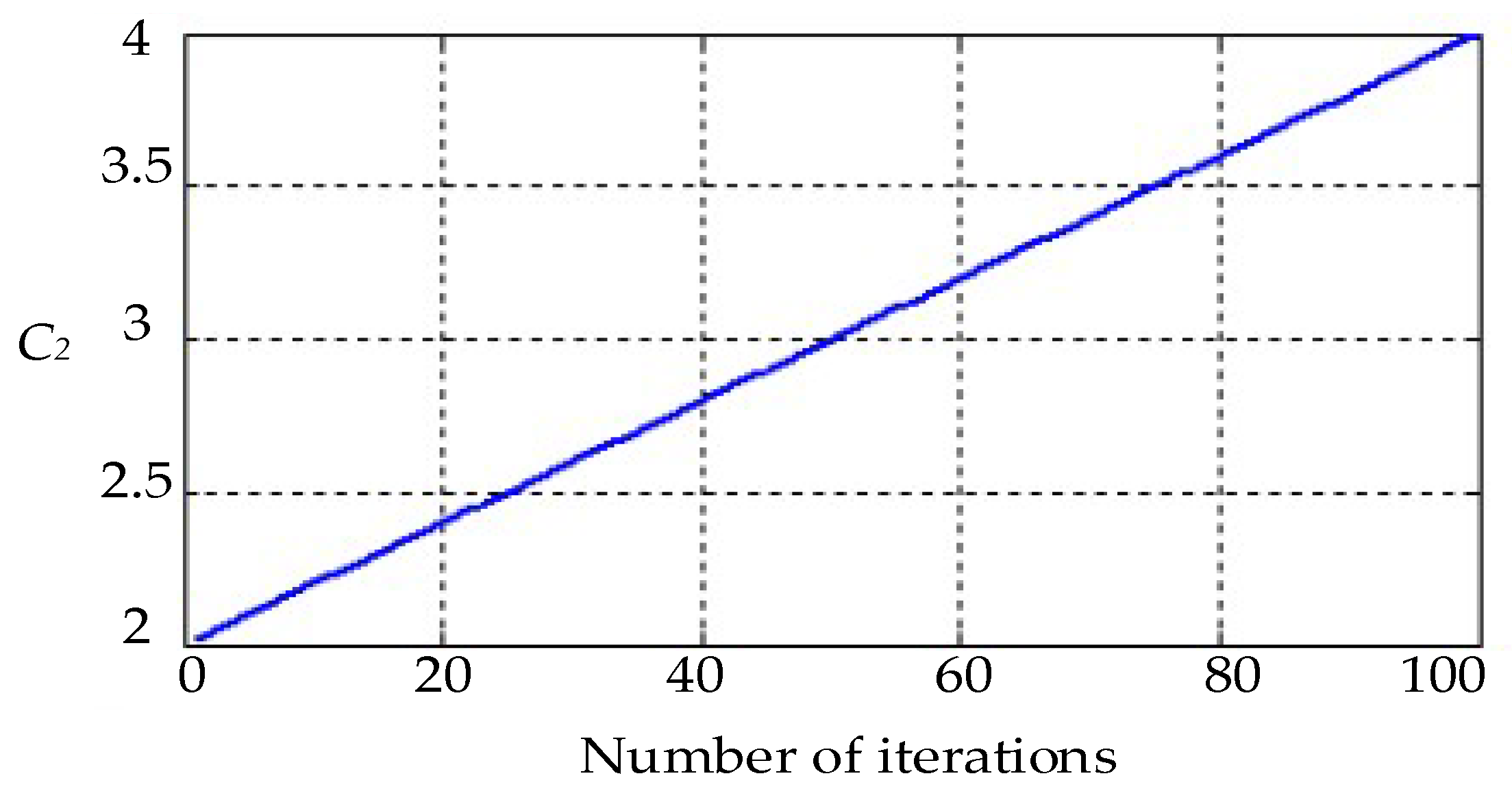
3.2. Improved Article Swarm Optimization Algorithm

The existing improved PSO [21] targets the weight value W of the traditional PSO. The modification method in Equation (3) enables particles to use larger moves in the early phase of iteration to perform the search, preventing it from failing to skip the local best solution due to overly small moves. However, as the number of iterations increases, since particles approximate the search of the actual MPP, if particle moves can be reduced, they can more precisely track the MPP. This modification method features the advantage of requiring fewer iterations compared to the traditional PSO and accurate tracking. However, it also has the disadvantage of failing to approximate the actual MPP in the early phase of iteration, resulting in a substantial increase in the number of iterations required [21].

$$W=W_{max}-\left(\left(W_{max}-W_{min}\right)\times {\left(\frac{j}{n}\right)}^2\right)$$

(3)

The weight value W parameters are described below.

• Upper limit of weight value (W_max): Represents the upper limit of the correlation with the moving distance of its own particles.
• Lower limit of weight value (W_min): Represents the lower limit of the correlation with the moving distance of its own particles.
• $j$: Represents the current number of iterations.
• n: Represents the highest number of iterations.

In terms of learning factors, since cognition learning factor C₁ uses Equation (4) to decrease the number of iterations, it means that, as the number of iterations increases, the best location value of its own particles as reference decreases; C₂ uses Equation (5) to increase the number of iterations, which means that, as the number of iterations increases, the global best location value of the particle is emphasized [21].

$$C_1=C_{1,max}-\left(\left(C_{1,max}-C_{1,min}\right)\times {\left(\frac{j}{n}\right)}^2\right)$$

(4)

$$C_2=C_{2,max}+\left(\left(C_{2,max}-C_{2,min}\right)\times {\left(\frac{j}{n}\right)}^2\right)$$

(5)

The learning factor parameters are described below.

• Upper limit of cognition learning factor (C_1,max): Represents the upper limit of the learning parameters related to its own particles.
• Lower limit of cognition learning factor (C_1,min): Represents the lower limit of the learning parameters related to its own particles.
• Upper limit of social learning factor (C_2,max): Represents the upper limit of the learning parameters related to other particles.
• Lower limit of social learning factor (C_2,min): Represents the lower limit of the learning parameters related to other particles.

3.3. Combining Artificial Bee Colony Algorithm

The ABC and PSO proposed in this study target the weight value W of PSO, which is modified using Equation (6). The advantage is that, during the particle search period, consistent moves will not cause convergence to slow down. The trend of the weight value W change is shown in Figure 3.

$$W=W_{\mathit{min}}+\left[\left(W_{\mathit{max}}-W_{\mathit{min}}\right)\times \mathit{rand}(•)\right]$$

(6)

where the definition of the weight value W parameters is the same as in the PSO proposed in Reference [21].

In terms of learning factors, cognition learning factor (C₁) is regarded as each individual bee, which, combined with ABC [22], is modified using Equation (7). During the tracking period, particles constantly calculate if a new solution is superior to the existing one. If so, the new solution is selected; if not, the existing solution is retained until the global best solution is found. On the other hand, C₂ is regarded as a bee colony, which is modified using Equation (8). The bees pass information to one another during the period of search in order to find the location of the best solution at the time, rather than searching blindly.

$$C_1=C_{1,max}-\left[\left(C_{1,max}-C_{1,min}\right)\times rand(•)\right]$$

(7)

$$C_2=C_{2,min}+\left[\left(C_{2,max}-C_{2,min}\right)\times \frac{j}{n}\right]$$

(8)

The trends of learning factor change are shown in Figure 4 and Figure 5. In terms of the parameter setting of the traditional PSO, the existing improved PSO, and the PSO proposed in this study, in order to avoid the three having overly similar parameters that affect subsequent experimental judgment, this paper set the upper limit and lower limit of weight value, cognition learning factor, and social learning as a two-fold difference, as shown in

Table 1. Parameter setting value of traditional particle swarm optimization (PSO).

Parameter Name	Parameter Setting Value
Number of particles	4
Number of iterations	100
Weight value W	0.4
Cognition learning factor C1	2
Social learning factor C2	2

and

Table 2. Parameter setting value of improved PSO proposed in Reference [21] and that proposed in this study.

Parameter Name	Parameter Setting Value
Number of particles	4
Number of iterations	100
Upper limit of weight value Wmax	0.9
Lower limit of weight value Wmin	0.2
Upper limit of cognition learning factor C1,max	4
Lower limit of cognition learning factor C1,min	2
Upper limit of social learning factor C2,max	4
Lower limit of social learning factor C2,min	2

. The definition of the learning factor parameters is also same as that in the PSO proposed in Reference [21]. Figure 6 shows the flowchart of the combined method of PSO and ABC.

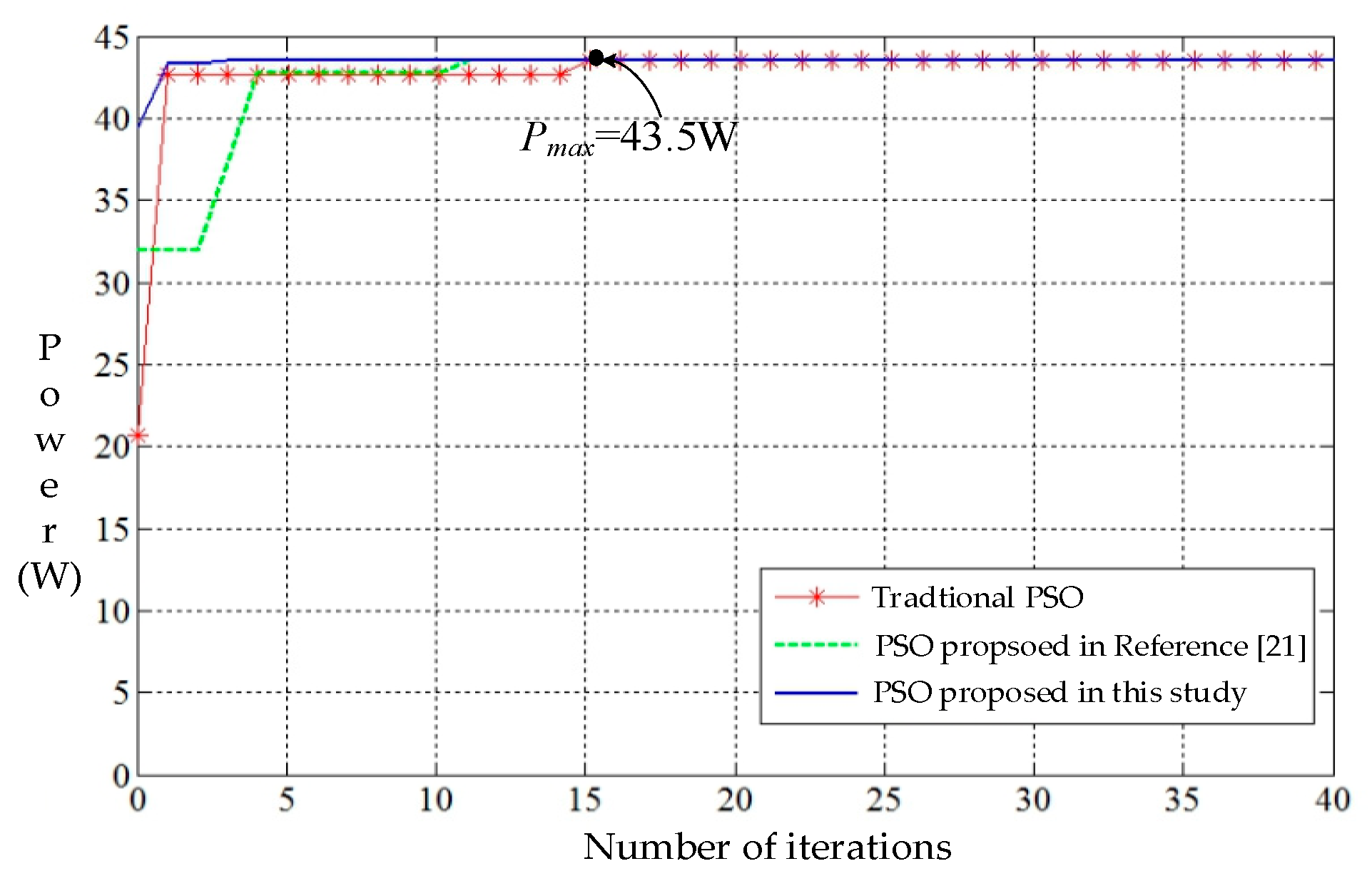
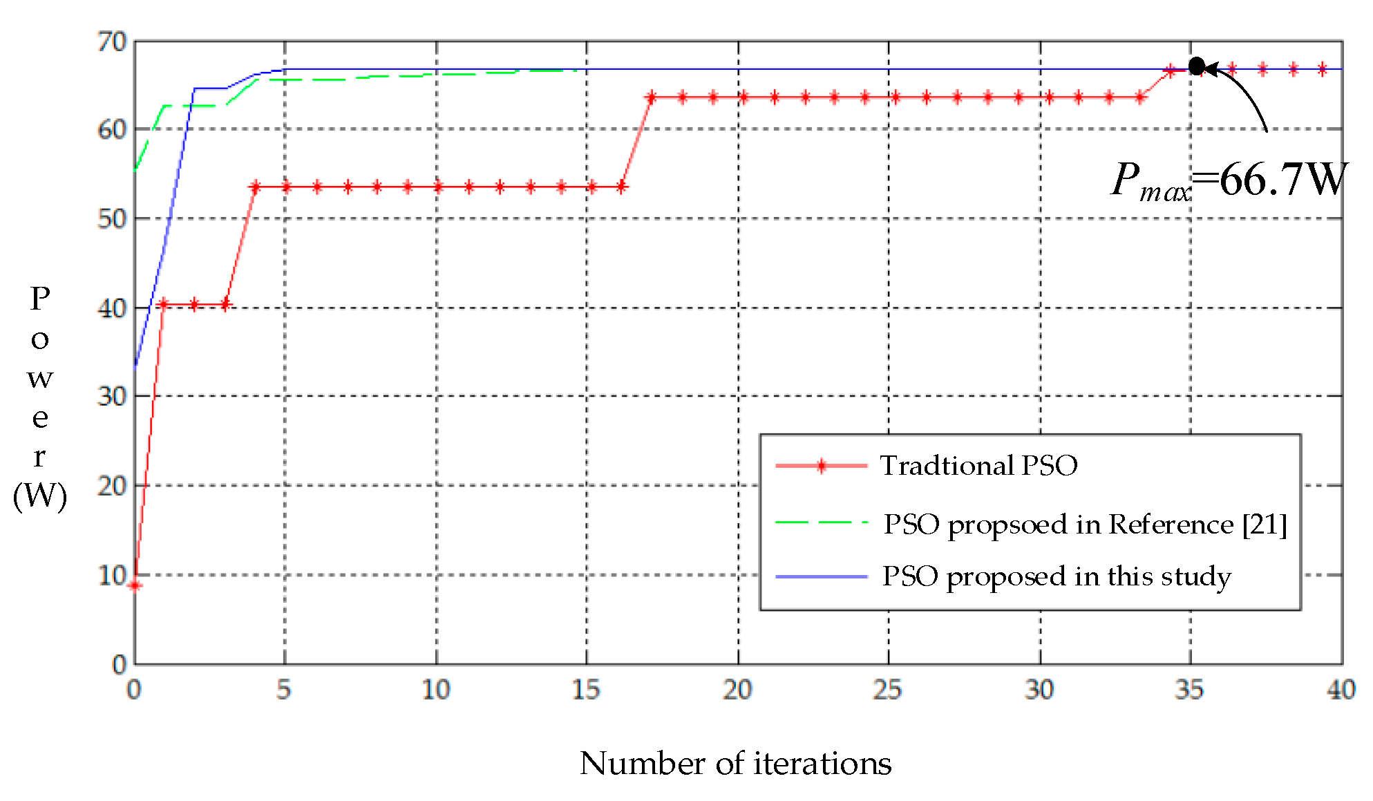
4. Simulation Results

The electric parameter specifications of the photovoltaic module adopted in this study are shown in

Table 3. Specifications of Sanyo HIP2717 Module.

Parameter	Value
Rated maximum output power ($P_{mp}$)	27.8 W
Current at maximum output power point ($I_{mp}$)	1.63 A
Voltage at maximum output power point ($V_{mp}$)	17.1 V
Short-circuit current ($I_{sc}$)	1.82 A
Open-circuit voltage ($V_{oc}$)	21.6 V

. Firstly, the HIP2717 photovoltaic module produced by SANYO (Moriguchi, Osaka, Japan) through the use of Solar Pro simulation software was used to form a characteristic curve with different parallel and series configurations and arrays in different shading ratios, as shown in

Table 4. Four shading conditions chosen.

Case	Shading Condition	P–V Curve Peaks
1	One-series, one-parallel connected: shading 0%	One peak
2	Two-series, one-parallel connected: shading 0% + shading 40%	Two peaks
3	Three-series, one-parallel connected: shading 0% + shading 30% + shading 70%	Three peaks
4	Four-series, one-parallel connected: shading 0% + shading 30% + shading 50% + shading 70%	Four peaks
5	Two-series, two-parallel connected: (shading 30% + shading 0%)//(shading 0% + shading 50%)	Two peaks

Note: Symbol “+” represented series connected; symbol “//” represents parallel connected.

. Then, MATLAB software was employed to simulate the traditional PSO, improved PSO proposed in Reference [21], and the combined ABC and PSO proposed in this study to carry out maximum power tracking and perform 100 maximum power tracking simulations. Finally, the average number of iterations using the three methods was calculated, and their strengths and weaknesses were compared.

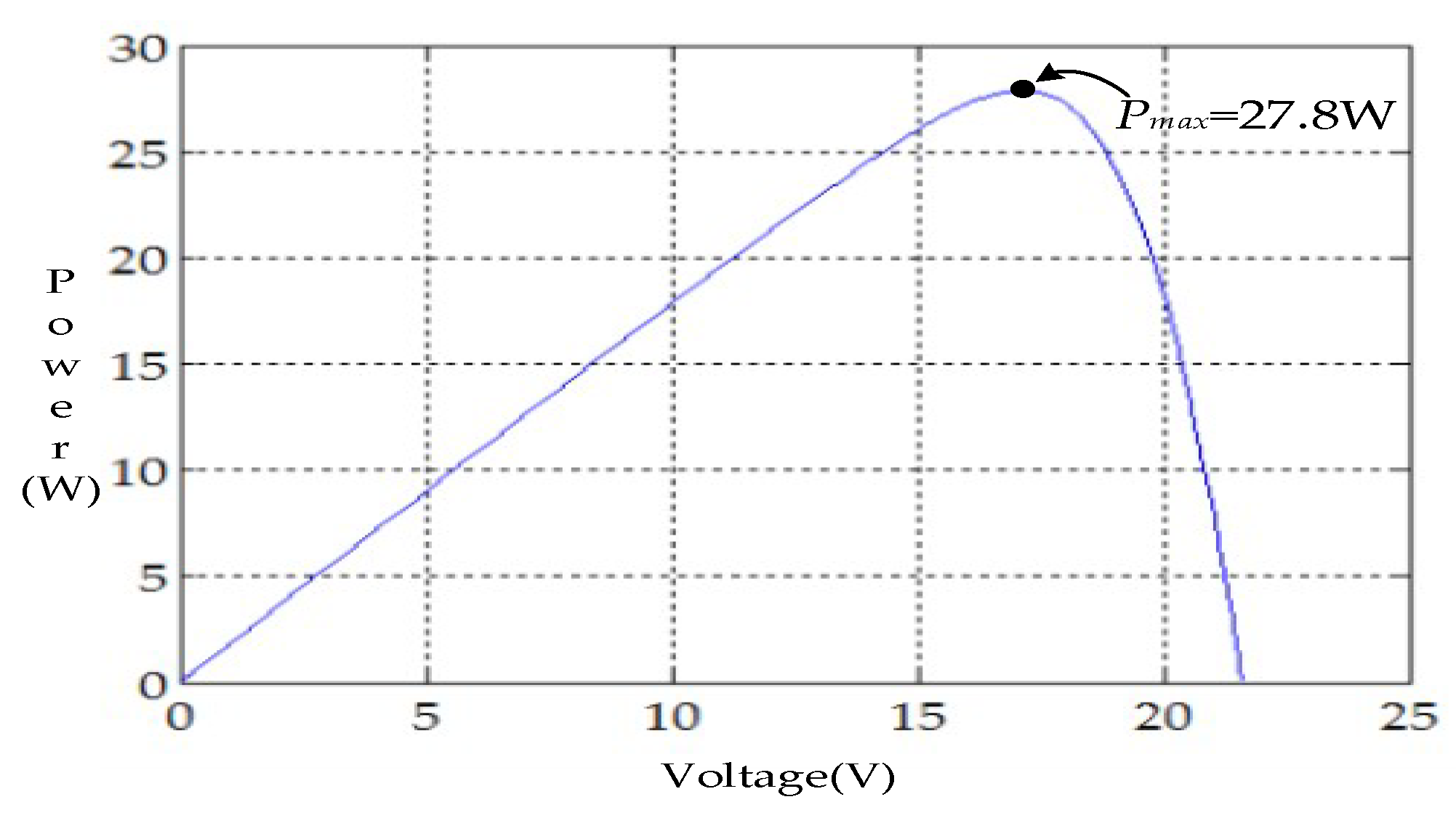
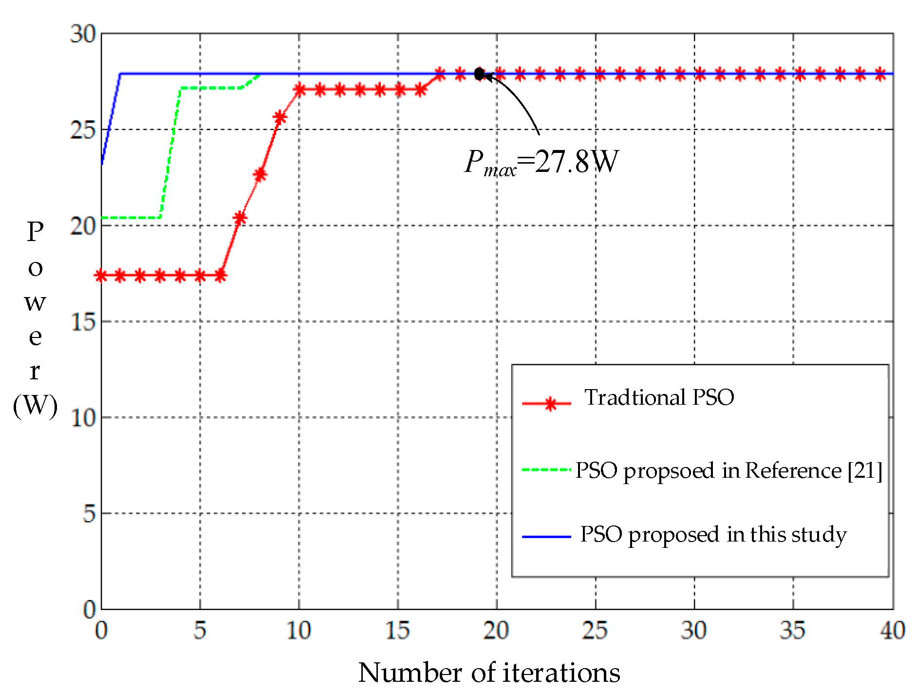
4.1. Case 1 (One-Series, One-Parallel: Shading 0%)

Figure 7 shows the P–V characteristic curve simulation of Case 1. When the photovoltaic module array is normal without shading, the maximum output power is about 27.8 W. Under this situation, the traditional PSO, the PSO proposed in Reference [21], and the PSO proposed in this study underwent maximum power tracking, and the tracking performance was compared. Based on the simulation results in Figure 8 using the three maximum power tracking methods, it was observed that the PSO proposed in this study had a faster tracking speed compared to the traditional PSO and the PSO proposed in Reference [21].

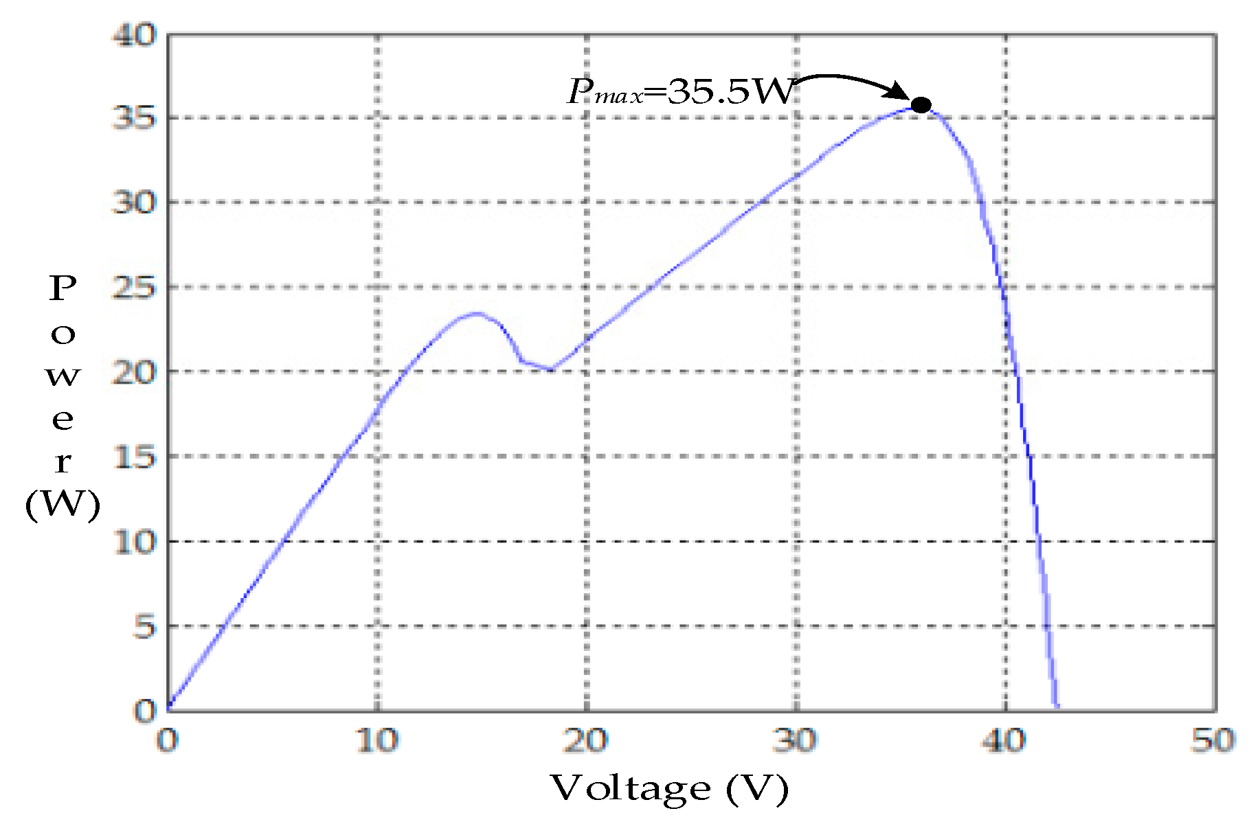
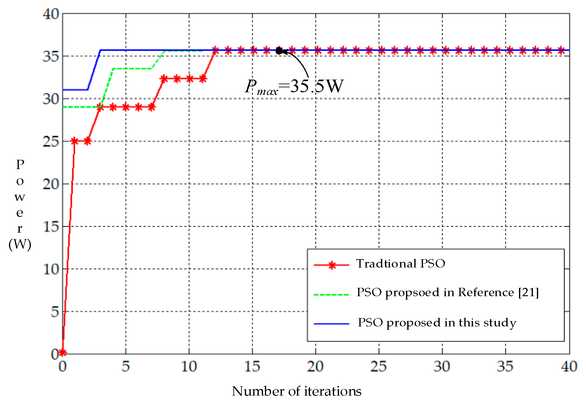
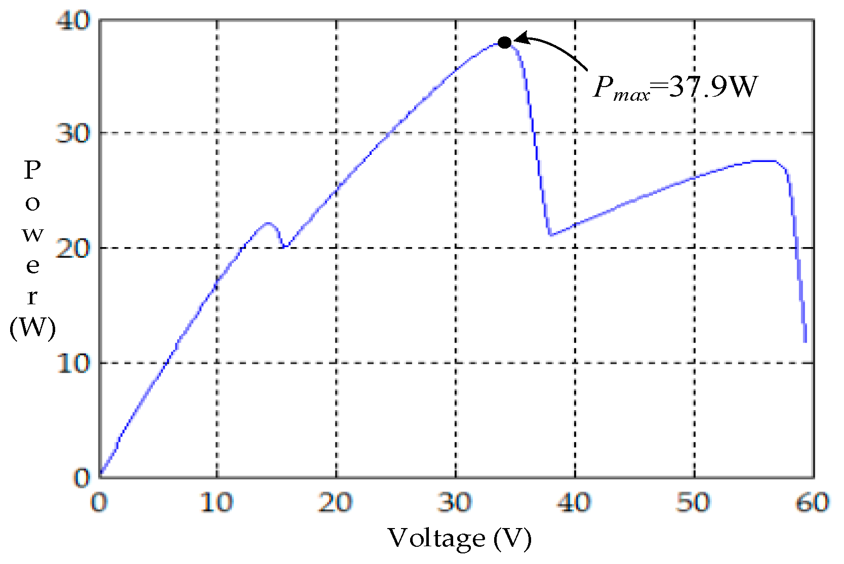
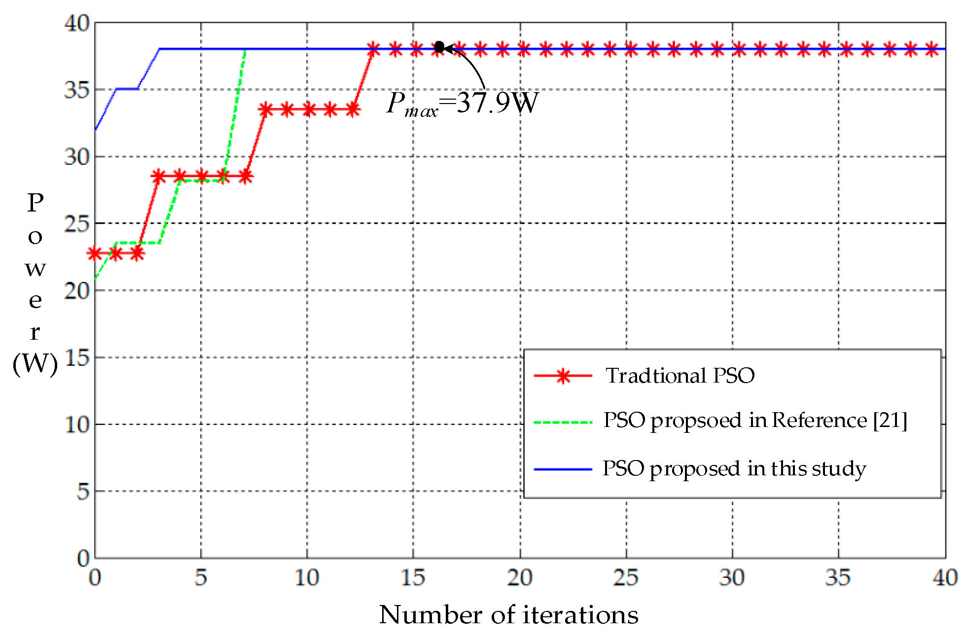
4.2. Case 2 (Two-Series One-Parallel: Shading 0% + Shading 40%)

Figure 9 shows the P–V characteristic curve of Case 2. One module in the photovoltaic module array is subject to 40% shading, resulting in a two-peak value in the P–V characteristic curve. The actual MPP is 35.5 W on the right side. Figure 10 shows the simulation results of maximum power tracking using three methods, namely the traditional PSO, the PSO proposed in Reference [21], and the PSO proposed in this study. Figure 10 shows that, although the three can track the actual MPP, they varied significantly in the number of iterations. The method proposed in this study can more quickly track the actual MPP.

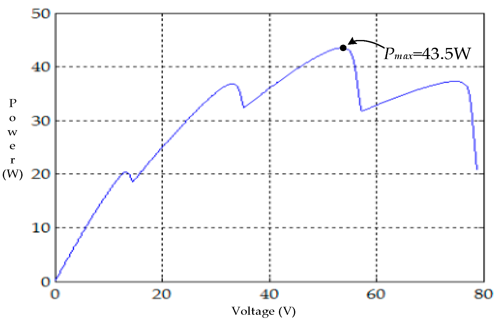
4.3. Case 3 (Three-Series One-Parallel: Shading 0% + Shading 30% + Shading 70%)

Figure 11 shows the simulation of the P–V characteristic curve in Case 3. Two modules in the photovoltaic module array are subject to 30% and 70% shading, resulting in a three-peak value in the characteristic curve. The actual maximum point is 37.9 W in the middle. Figure 12 shows the simulation results using maximum power tracking methods, namely the traditional PSO, the PSO in Reference [21], and the PSO proposed in this study. Figure 12 shows that, when the traditional PSO is adopted, the speed of skipping from the local solution is slower, and more time is needed to track the actual MPP (37.9 W); meanwhile, although the improved PSO proposed in Reference [21] has a faster tracking speed compared to the traditional PSO, it has the tendency to be trapped in the local solution. As for the PSO proposed in this study, in addition to faster skipping from the local solution, the MPP tracking precision (37.9 W) and speed are also better compared to the other two methods.

4.4. Case 4 (Four-Series One-Parallel: Shading 0% + Shading 30% + Shading 50% + Shading 70%)

Figure 13 shows the implementation of the P–V characteristic curve of Case 4. Due to an increase in the number of parallel and series connections in the photovoltaic module array, three modules were subject to 30%, 50%, and 70% shading, resulting in a four-peak value in the P–V characteristic curve. The actual MPP is at the third peak value. Figure 14 shows the simulation results using the maximum tracking methods, namely the traditional PSO, the PSO proposed in Reference [21], and the PSO proposed in this study. Figure 14 shows that, when the traditional PSO is adopted, although the MPP can be tracked, it is trapped in the local solution, resulting in a slow tracking speed. As for the PSO proposed in Reference [21], trapping in the local solution also occurred. The PSO proposed in this study was not trapped in the local solution. Hence, its tracking speed is significantly superior to the traditional PSO and the PSO proposed in Reference [21].

4.5. Case 5 (Two-Series Two-Parallel: (Shading 30% + Shading 0%)//(Shading 0% + Shading 50%))

Figure 15 shows the simulation of the P–V characteristic curve in Case 5. Two modules in the photovoltaic module array are subject to 30% and 50% shading, resulting in a two-peak value in the P–V characteristic curve. The actual MPP is 66.7 W on the right side. Figure 16 shows the simulation results using maximum tracking methods, namely the traditional PSO, the PSO proposed in Reference [21], and the PSO proposed in this study. Figure 16 shows that the traditional PSO requires a higher number of iterations to track the actual maximum power point, while the PSO proposed in Reference [21] and the PSO proposed in this study can quickly track the actual MPP. The tracking performance of the proposed method is also superior to the method proposed in Reference [21].

4.6. Case Simulation Result Comparison and Analysis

The stable values shown in Figure 8, Figure 10, Figure 12, Figure 14, and Figure 16 are all the optimal solutions using the traditional PSO, the PSO proposed in Reference [21], and the PSO proposed in this study, and they were all obtained within the highest number of iterations we set (100). The number of iterations for the three optimization methods to obtain the optimal value in each case is listed in

Table 5. Number of iterations for various optimization methods to obtain the optimal values for the five cases.

Case	Number of Iterations
	Traditional PSO	PSO Proposed in Reference [21]	PSO Proposed in this Study
1	17	5	2
2	12	6	3
3	11	7	2
4	15	11	3
5	34	15	5

. As can be seen in Table 5, the optimal values obtained using different optimization methods are within the set number of iterations in each case.

The five cases selected in this study underwent 100 simulations using the traditional PSO, the PSO proposed in Reference [21], and the PSO proposed in this study. Then, the number of iterations was tallied and compiled, as shown in

Table 6. Comparison of simulation results of five case simulations selected.

Case	Number of P–V Curve Peaks	Average Number of Iterations/Standard Deviation
		Traditional PSO	PSO Proposed in Reference [21]	PSO Proposed in this Study
1	One peak	8.58/3.95	7.2/3.16	6.45/2.80
2	Two peaks	18.63/9.21	11.5/6.54	8.4/3.42
3	Three peaks	31.14/12.21	24.94/6.60	14.05/4.2
4	Four peaks	31.27/12.99	18.3/8.69	14.38/4.99
5	Two peaks	22.7/5.66	17.48/4.42	10.8/3.13

. The number of iterations required by the proposed PSO in multiple simulations of the cases was less than that of the traditional PSO and the PSO proposed in Reference [21].

In addition, it was also found that the traditional PSO and the PSO proposed in Reference [21] had an unideal average number of iterations in multiple simulations of Case 3, mainly because the multi-peak values had a highly approximate local solution, resulting in the traditional PSO and the PSO proposed in Reference [21] failing to skip the local solution; thus, a higher number of iterations were needed to track the actual MPP. The standard deviations of the needed number of iterations for five cases using the traditional PSO, the PSO proposed in Reference [21], and the PSO proposed in this study are shown in Table 6. It can be observed that the standard deviation of the PSO proposed in this study is smaller than the traditional PSO method and the PSO proposed in Reference [21]. It indicates that the number of iterations of the proposed method was almost the same each time it reached the actual MPP, which means that the time tracked by the proposed method to fall into the local MPP is very short. Therefore, it can provide a faster tracking speed.

5. Conclusions

This paper modified the algorithm proposed in the traditional PSO and that in Reference [21], combining it with ABC to give rise to the development of an optimized PSO algorithm used to perform the maximum power tracking of a photovoltaic module array. The PSO weight values, cognition learning factors, and swarm factor parameters proposed in this study changed with the number of iterations. Therefore, the number of iterations could be reduced. The simulation results prove that, for the photovoltaic module array with partial module shading, the ABC combined with PSO can more precisely and quickly track the actual MPP of the photovoltaic module array compared to the traditional PSO and the PSO proposed in Reference [21]. Moreover, the combined method of ABC and PSO can reduce the standard deviation under different shading cases of photovoltaic module arrays, resulting in an even smaller value than the deterministic techniques.

From the simulation results, it can be seen that the optimization method proposed in this paper needs fewer iterations to track the global MPP under different shading conditions. In addition, the number of iterations required in different shading conditions is not significantly different. It means that the optimization method proposed in this study prevents it from falling easily into a local MPP; thus, it can provide a faster tracking speed.

References

1. Masoum, M.A.S.; Sarvi, M. Voltage and current based MPPT of solar arrays under variable insolation and temperature conditions. In Proceedings of the 43th International Universities Power Engineering Conference (UPEC), Padova, Italy, 1–4 September 2008; pp. 39–43. [Google Scholar]
2. Masoum, M.A.S.; Dehbonei, H.; Fuchs, E.F. Theoretical and experimental analyses of photovoltaic systems with voltage and current-based maximum power-point tracking. IEEE Trans. Energy Conver. 2002, 17, 514–522. [Google Scholar] [CrossRef]
3. Esram, T.T.; Chapman, P.L. Comparison of photovoltaic array MPP tracking techniques. IEEE Trans. Energy. Conver. 2007, 22, 439–449. [Google Scholar] [CrossRef]
4. Femia, N.; Granozio, D.; Petrone, G.; Vitelli, M. Predictive and adaptive MPPT perturb and observe method. IEEE Trans. Aero. Elec. Sys. 2007, 43, 934–950. [Google Scholar] [CrossRef]
5. Liu, F.; Duan, B.; Kang, Y. A variable step size INC MPPT method for PV systems. IEEE Trans. Ind. Electron. 2008, 55, 2622–2628. [Google Scholar]
6. Wang, Y.J.; Hsu, P.C. Analytical modeling of partial shading and different orientation of photovoltaic modules. IET. Renew. Power. Gen. 2010, 4, 272–282. [Google Scholar] [CrossRef]
7. Kottas, T.L.; Boutalis, Y.B.; Karis, A.D. New MPP tracker for PV arrays using fuzzy controller in close cooperation with fuzzy cognitive networks. IEEE Trans. Energy. Conver. 2006, 21, 793–803. [Google Scholar] [CrossRef]
8. Ramaprabba, R.; Gothandaraman, V.; Kanimozhi, K.; Divya, R.; Mathur, B.L. Maximum power point tracking using GA-optimized artificial neural network for solar PV system. In Proceedings of the 1st International Conference on Electrical Energy Systems (ICEES), Newport Beach, CA, USA, 3–5 January 2011; pp. 264–268. [Google Scholar]
9. Veerachary, T.; Senjyu, T.; Uezato, K. Neural-network-based maximum-power-point tracking of coupled-inductor interleaved-boost-converter-supplied PV system using fuzzy controller. IEEE Trans. Ind. Electron. 2003, 50, 749–758. [Google Scholar] [CrossRef]
10. Sundareswaran, K.; Senjyu, T.; Nayak, P.S.R.; Simon, S.P.; Palani, S. Enhanced energy output from a PV system under partial shaded conditions through artificial bee colony. IEEE Trans. Energy. Conver. 2015, 6, 198–209. [Google Scholar] [CrossRef]
11. Chao, K.H.; Chiu, C.L. Design and implementation of an intelligent maximum power point tracking controller for photovoltaic systems. Int. Rev. Electr. Eng. 2012, 7, 3759–3768. [Google Scholar]
12. Kvasov, D.E.; Menniti, D.; Pinnarelli, A.; Sergeyev, Y.D.; Sorrentino, N. Tuning fuzzy power-system stabilizers in multi-machine systems by global optimization algorithms based on efficient domain partitions. Electr. Power Syst. Res. 2008, 78, 1217–1229. [Google Scholar] [CrossRef]
13. Kvasov, D.E.; Sergeyev, Y.D. Lipschitz global optimization methods in control problems. Automat. Rem. Contr. 2013, 78, 1435–1448. [Google Scholar] [CrossRef]
14. Kvasov, D.E.; Mukhametzhanov, M.S. Metaheuristic vs. deterministic global optimization algorithms: The univariate case. Appl. Math. Comput. 2018, 318, 245–259. [Google Scholar] [CrossRef]
15. Sergeyev, Y.D.; Kvasov, D.E.; Mukhametzhanov, M.S. On the efficiency of nature-inspired metaheuristics in expensive global optimization with limited budget. Sci. Rep. 2018, 8, 453. [Google Scholar] [CrossRef] [PubMed]
16. Solar Pro official website. Available online: https://www.lapsys.co.jp/english/products/download.html (accessed on 12 April 2019).
17. Kennedy, J.; Eberhart, R.C. Particle swarm optimization. In Proceedings of the IEEE International Conference on Neural Networks (ICNN), Perth, Australia, 27 November–1 December 1995; pp. 1942–1948. [Google Scholar]
18. Eberhart, R.C.; Kennedy, J. A new optimizer using particle swarm theory. In Proceedings of the sixth International Symposium on Micro Machine and Human Science (MHS), Nagoya, Japan, 4–6 October 1995; pp. 39–43. [Google Scholar]
19. Srinivasan, D.; Loo, W.H.; Cheu, R.L. Traffic incident detection using particle swarm optimization. In Proceedings of the IEEE International Conference on Swarm Intelligence Symposium (SIS), Indianapolis, IN, USA, 26 April 2003; pp. 144–151. [Google Scholar]
20. Han, W.H.; Yang, P.; Ren, H.; Sun, J. Comparison study of several kinds of inertia weights for PSO. In Proceedings of the IEEE International Conference on Progress in Informatics and Computing (PIC), Shanghai, China, 10–12 December 2010; pp. 280–284. [Google Scholar]
21. Chang, L.Y.; Chung, Y.N.; Chao, J.J. Smart global MPP tracking controller of photovoltaic module arrays. Energies 2018, 11, 567. [Google Scholar] [CrossRef]
22. Liu, Y.; Ling, X.; Liang, Y. Improved artificial bee colony algorithm with mutual learning. J. Syst. Eng. Electron. 2012, 2, 265–275. [Google Scholar] [CrossRef]
Figure 1. Simulated I–V characteristic curve when different modules in the four-series and one-parallel connected module array have 25% shading.
Electronics 08 00603 g001
Figure 2. Simulated P–V characteristic curve when different modules in the four-series and one-parallel connected module array have 25% shading.
Electronics 08 00603 g002
Figure 3. Trend of weight W change combining artificial bee colony (ABC) and particle swarm optimization (PSO).
Electronics 08 00603 g003
Figure 4. Trend of cognition learning factor C1 combining ABC and PSO.
Electronics 08 00603 g004
Figure 5. Trend of social learning factor C2 combining ABC and PSO.
Electronics 08 00603 g005
Figure 6. Flowchart combining ABC and PSO.
Electronics 08 00603 g006
Figure 7. Simulation of P–V characteristic curve in Case 1.
Electronics 08 00603 g007
Figure 8. Comparison reuslts of maximum power tracking in Case 1 using the traditional PSO, the improved PSO in Reference [21], and the PSO proposed in this study.
Electronics 08 00603 g008
Figure 9. Simulation of P–V characteristic curve in Case 2.
Electronics 08 00603 g009
Figure 10. Comparison reuslts of maximum power tracking in Case 2 using the traditional PSO, the improved PSO in Reference [21], and the PSO proposed in this study.
Electronics 08 00603 g010
Figure 11. Simulation of P–V characteristic curve in Case 3.
Electronics 08 00603 g011
Figure 12. Comparison results of maximum power tracking in Case 3 using the traditional PSO, the improved PSO proposed in Reference [21], and the PSO proposed in this study.
Electronics 08 00603 g012
Figure 13. Simulation of P–V characteristic curve in Case 4.
Electronics 08 00603 g013
Figure 14. Comaprison resutls of maximum power tracking in Case 4 using the traditional PSO, the PSO in Reference [21], and the PSO proposed in this study.
Electronics 08 00603 g014
Figure 15. Simulation of P–V characteristic curve in Case 5.
Electronics 08 00603 g015
Figure 16. Comparison reuslts of maximum tracking in Case 5 using the traditional PSO, the improved PSO proposed in Refference [21], and the PSO proposed in this study.
Electronics 08 00603 g016