Time Series Analysis to Predict End-to-End Quality of Wireless Community Networks ^†

Abstract

Community Networks have been around us for decades being initially deployed in the USA and Europe. They were designed by individuals to provide open and free “do it yourself” Internet access to other individuals in the same community and geographic area. In recent years, they have evolved as a viable solution to provide Internet access in developing countries and rural areas. Their social impact is measurable, as the community is provided with the right and opportunity of communication. Community networks combine wired and wireless links, and the nature of the wireless medium is unreliable. This poses several challenges to the routing protocol. For instance, Link-State routing protocols deal with End-to-End Quality tracking to select paths that maximize the delivery rate and minimize traffic congestion. In this work, we focused on End-to-End Quality prediction by means of time-series analysis to foresee which paths are more likely to change their quality. We show that it is possible to accurately predict End-to-End Quality with a small Mean Absolute Error in the routing layer of large-scale, distributed, and decentralized networks. In particular, we analyzed the path ETX behavior and properties to better identify the best prediction algorithm. We also analyzed the End-to-End Quality prediction accuracy some steps ahead in the future, as well as its dependency on the hour of the day. Besides, we quantified the computational cost of the prediction. Finally, we evaluated the impact of the usage for routing of our approach versus a simplified OLSR (ETX + Dijkstra) on an overloaded network.

1. Introduction

Community Networks (CNs) are large-scale, distributed, and decentralized networking infrastructures composed of several nodes, links, and services, where the resources are made available to a group of people living in the same area. Sometimes, these networks are referred to as “the Internet by the People for the People” [1], and offer a solution to the critical problem of closing the digital divide in the developing world [2]. CNs [3] are structured to be open, free, and to respect network neutrality. Such networks rely on the active participation of local communities in the design, development, deployment, and management of shared infrastructure as a common resource, owned by the community, and operated in a democratic fashion. Community networks can be operationalized, entirely or partly, through individuals and local stakeholders, NGOs, private sector entities, and/or public administrations.

This kind of networks are extremely diverse and dynamic, because they are composed of decentralized nodes and they mix wired and wireless technologies, several routing schemes, and diverse services and applications [4]. In addition, they grow dynamically with regards to the number of links, their capacity, and services provided. Some relevant examples of CNs include guifi.net [5], FunkFeuer [6], or AWMN [7]. Among many others, the guifi.net CN exemplifies how communities can develop their own network infrastructures as a commons [8], using several interconnected Wireless Mesh Networks. This results in a large-scale and heterogeneous network which uses diverse routing protocols in several network zones.

Community Networks characteristics (large, heterogeneous, dynamic, and decentralized) raise multiple challenges of interest for researchers [9]. One of the most important challenges is the effect of the asymmetrical features and unreliability of wireless communications on network performance and routing protocols. Many metric-based routing protocols for wireless mesh networks that track Link Quality (LQ) and select higher-quality links have been proposed to minimize traffic congestion and maximize delivery rate [10,11,12,13]. Hence, when routing packets through an unreliable network, LQ tracking is definitely a key method to apply. Moreover, routing algorithms should avoid weak links as soon as possible [14], and whenever possible [15]. LQ estimation [16] (or prediction [17]) approach increases the improvements achieved by LQ tracking in routing performance. Usually, real-time metrics do not provide enough information to detect the degradation or activation of a link at the right time. Therefore, prediction techniques are needed to foresee LQ changes and take the appropriate measures.

Path Awareness [18] is a new Internet architectural-property proposal. The evolution of Internet allows different paths with diverse properties. The endpoints must be aware of these path properties (provided by the network), to make informed decisions about the paths to use. Prediction of path changes can improve local node routing decisions, since it can provide the node with an estimation about the future local and remote events.

End-to-End Quality (EtEQ) or Path Quality extends the Link Quality concept to the full communication path (between sender and receiver) and it is computed based on the quality of the individual links that conform the communication path. In [19], we analyzed if our previous work on LQ [20] is applicable to the full communication path (EtEQ tracking and prediction) and we determined what differences exist between individual LQ and EtEQ. To the best of our knowledge, no previous work has explored EtEQ prediction in the routing layer of large-scale, distributed, and decentralized systems. In this paper, we extend our previous work [19] by analyzing the Path and Link behavior and determining the computational cost of the EtEQ prediction.

Our proposal focuses on reducing the computational cost of EtEQ prediction in order to allow direct execution in the routers, contrary to other works that use Machine Learning and Deep Learning to predict routing information and routing tables [21,22]. To the best of our knowledge, all previous works have a high computational cost and require dedicated hardware. Routers, particularly those used in community networks, have very limited hardware. Additionally, many of the proposed computation techniques (Machine Learning and Deep Learning based) are offline, outside the network, and there is an important cost of moving the information from the network to the computing resources. Some works [23] allow them to execute online Machine Learning algorithms inside a router with low computational cost, but we believe that these algorithms are devoted to compete in CPU with the routing algorithms. Conversely, we prioritize routing decision over machine learning training for faster response times. Our samples show small topology changes, so we can arrange the machine learning training over a longer period of time, resulting in low effective computational cost.

The main contributions of this work are the following:

• A detailed analysis of path properties behavior in Wireless Mesh Community Networks (WMCNs) shows that Path Quality prediction is possible and meaningful.
• Time-Series analysis is used to estimate EtEQ in the routing layer of real-world WMCNs.
• Clear evidence that EtEQ values computed through Time-Series algorithms can make accurate predictions in WMCNs is provided.
• A detailed analysis of the prediction accuracy for the next step considering also the hour of the day, and for some steps ahead in the future is presented.
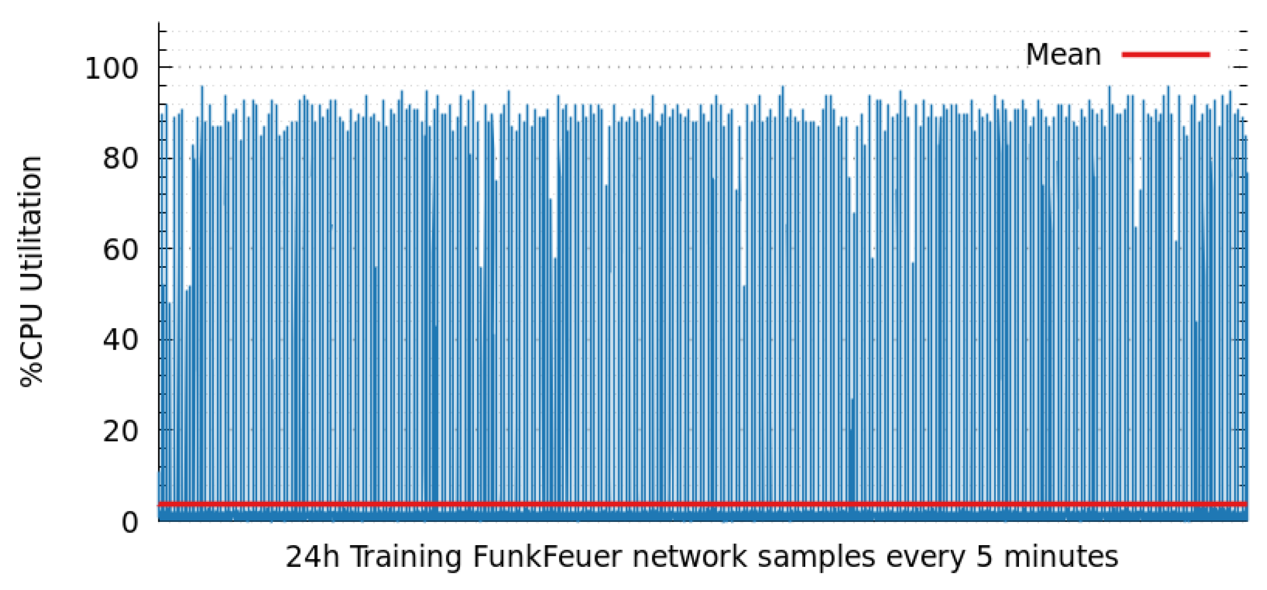
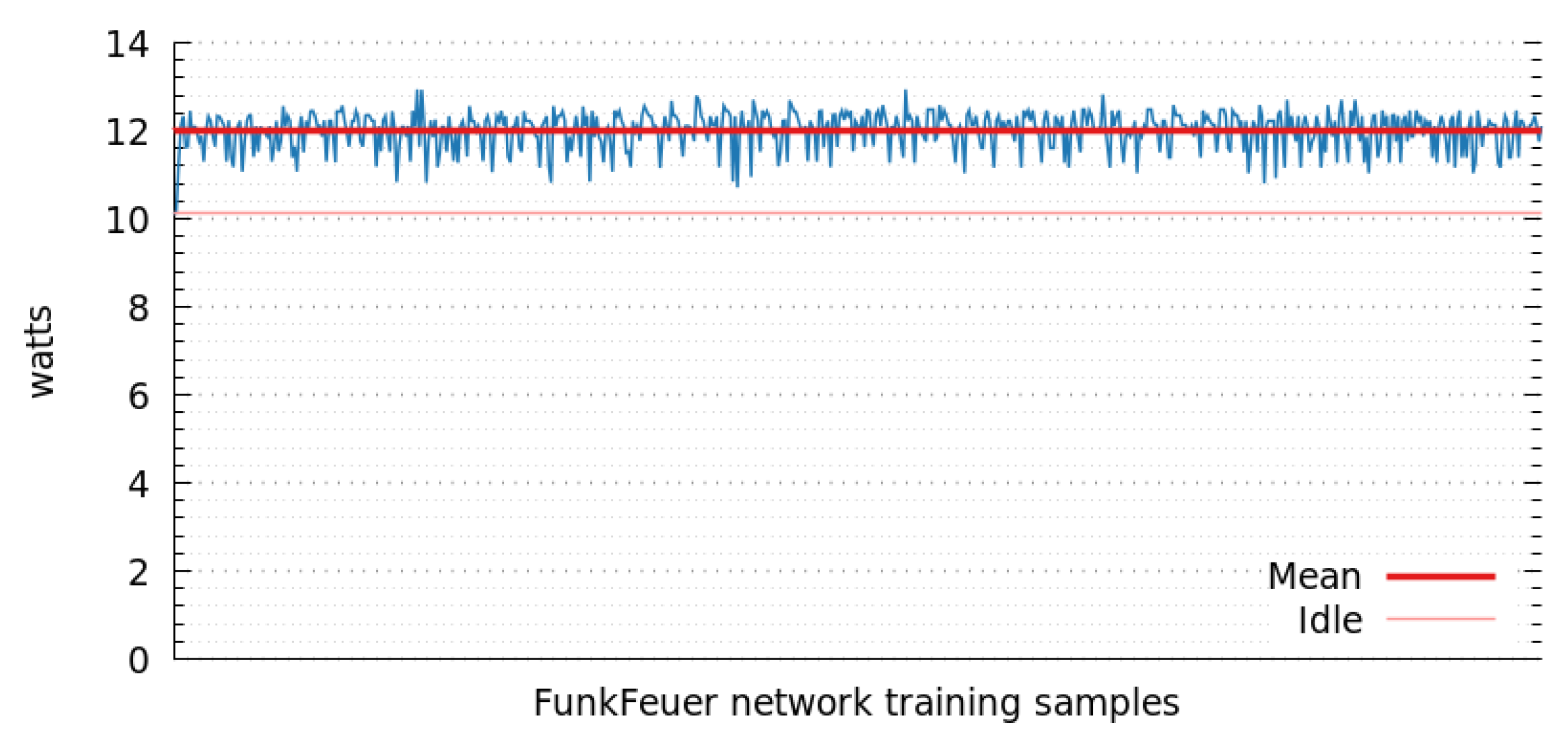
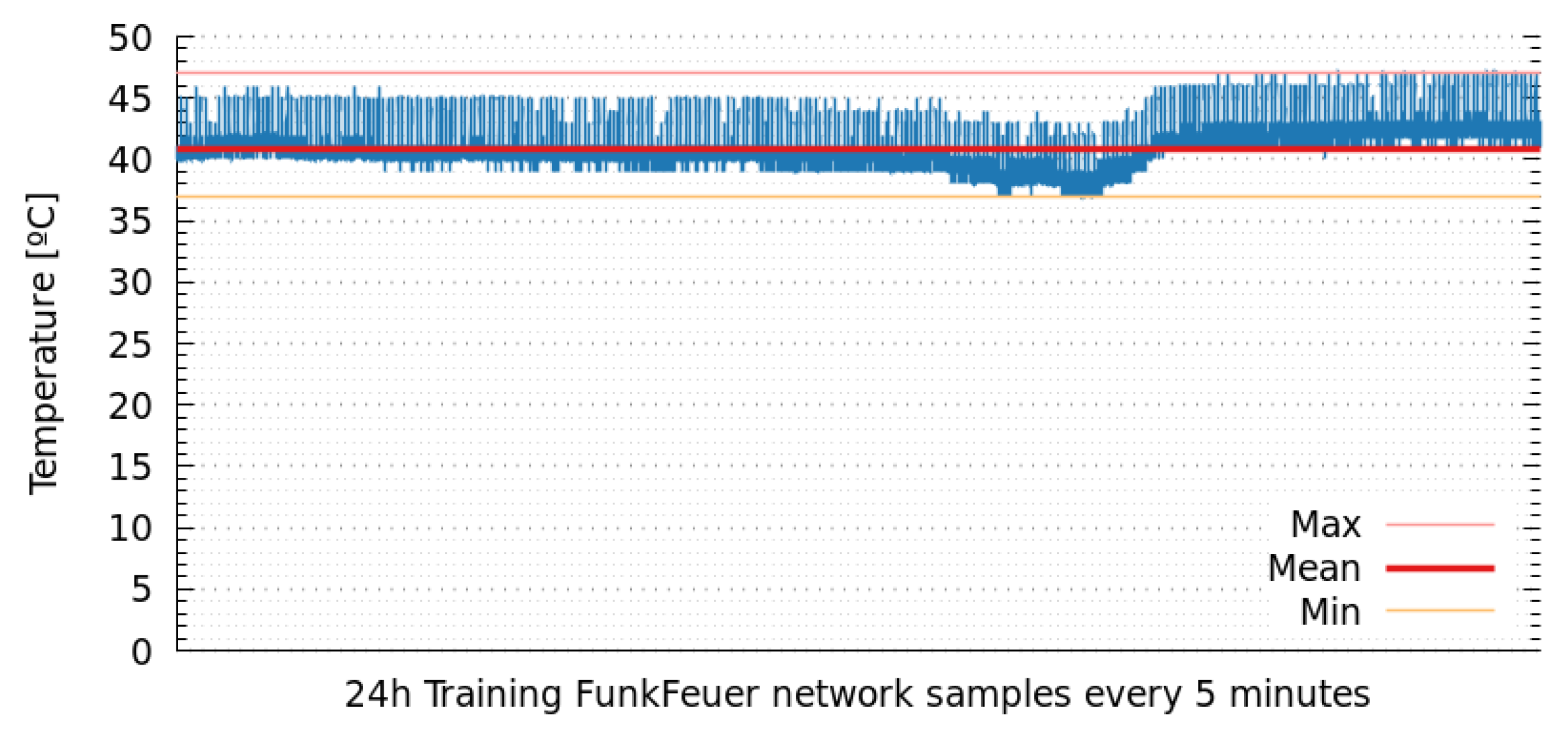
• An analysis of the computational cost of the prediction in terms of CPU utilization, energy consumption and temperature to confirm that the prediction can be executed directly in the routers is presented.
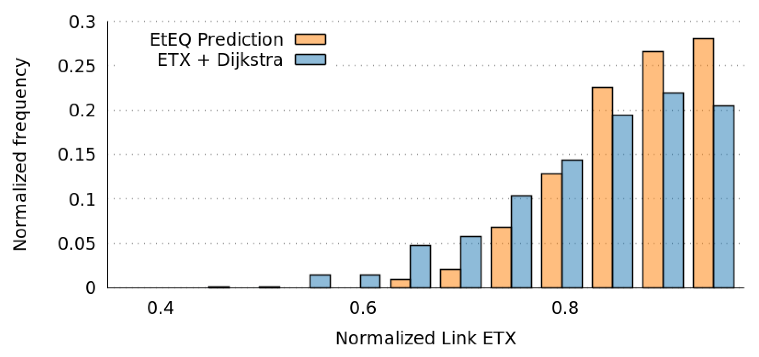
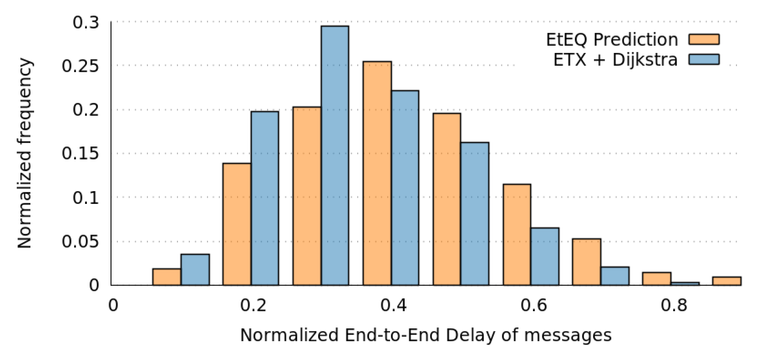
• A detailed analysis of a use case shows the behavior of two orthogonal routing strategies, in terms of Packet Delivery Ratio, ETX of links, and End-to-End Delay.

This paper is structured as follows. Section 2 overviews prediction in computer networks focused on link/path quality prediction in WMCN. Section 3 describes and analyses the dataset assumed in this work and introduces our proposal by showing the EtEQ behavior of a WMCN. Section 4 describes the experiments made to show the value of EtEQ prediction and it also analyzes the computational cost of the prediction. Finally, Section 6 provides some conclusions and future work.

2. Link and End-to-End Quality Prediction in Heterogeneous Networks

Prediction techniques have been applied in several ways such as routing traffic reduction [24,25,26], energy efficient routing [27,28,29], or LQ estimation.

LQ tracking has been previously applied in several scenarios in different ways [10,11,12,13] to select higher quality links that maximize delivery rate and minimize traffic congestion. Link Quality Estimators (LQE) [16,17] are in charge of measuring the quality of the links between nodes based on physical or logical metrics. Physical metrics focus on the received signal quality [30,31,32], and logical metrics focus on the percentage of lost packets [10,33,34]. All these metrics can be used by LQE in isolation or as a combination of some of them [16,17,35] to select the more suitable neighbor nodes when making routing decisions. LQ prediction is used in addition to LQ tracking to determine beforehand which links are more likely to change their behavior. Although LQ prediction is not identical to EtEQ prediction, some of the above techniques can be very similar [10,30,31,33,34,35]. This relationship is even more direct in the case of ETX EtEQ, studied in this paper, which is a linear function of the ETX LQ. As a result, the routing layer can take better decisions at the appropriate moment.

Prediction of path changes can improve local node routing decisions, since it can provide the node with an estimation about the future local and remote events. End-to-End Quality has not been widely considered in the past. In fact, the main efforts have been focused on determining the cost of a single link, and then extended to the full path by assuming the cost of a path as the sum of costs of several links. For instance, MARA [36] has been proposed to make more accurate routing decisions by combining route quality evaluation and automatic rate selection. EER [37] claims that the total cost of a path cannot be expressed as a linear sum of individual link costs. Therefore, variations of this simple formulation are proposed, such as incorporating error rate in the link cost. This achieves significant energy savings compared to traditional minimum energy approaches. ETOP [38] has been proposed as a path metric to determine reliable end-to-end packet delivery. Finally, EED/WEED [39] is another approach that was designed as a link/path metric to select paths with minimum end-to-end delay and high network throughput, but considering load balancing of routing. In any case, there is no work concerning prediction of Path Quality in WMCNs.

Some relevant works must be paid special attention as they are related to our study, namely those of Wang et al. [40], Maccari and Cigno [41], Cunha et al. [42], and Millán et al. [20]. Wang et al. [40] introduced the MetricMap mechanism, which is fundamentally a routing protocol for WSNs that uses a learning-enabled method for LQ assessment. Based on the observation that high traffic rates make tracking LQs more difficult, this protocol uses prediction methods to estimate them in advance. Results show that MetricMap can achieve a significant improvement on the data delivery rate in high traffic-rate applications. Maccari and Lo Cigno [41] considered the FunkFeuer network focusing on link-layer properties, topological patterns, and routing performance. They analyzed the quality of the routes, and proposed a couple of techniques to select the MPR nodes in the OLSR protocol. Cunha et al. [42] proposed a simple strategy for improving routing in the Internet domain, which moves in two ways: first, it detects path changes (NN4 approach) and then it remaps these paths once a change is detected (DTRACK approach). Results show that NN4 is not highly accurate, but it demonstrates the potential of prediction to improve the routing layer when making routing decisions. Millán et al. [20] analyzed the behavior of LQ prediction in the routing layer of large-scale, distributed, and decentralized systems, composed of many nodes, links, content, and services. Their main contributions are: (1) the use of time-series (TS) analysis to estimate LQ in the routing layer for real-world WMCN; (2) the detailed evaluation of results, assuming several learning algorithms to show the potentiality of TS analysis for estimating LQ in short and long term; and (3) the evidence that LQ computed from TS can be used to accurately predict future values in WMCN. In the same way, Lowrance and Lauf [43] proposed applying an online learning algorithm that progressively updates the model, and to perform evaluations in a mobile environment, with more variability than the stationary network used in [20].

There are two different approaches for applying prediction to routing [21,22]: (1) new routing algorithms based on Machine Learning and Deep Learning; and (2) classical routing algorithms but with Machine Learning based metrics. These two approaches are widely used in other environments, for example Software-Defined Networking (SDN). In this work, we focus on the latter approach.

Several authors deal with the Machine Learning and Deep Learning Based Routing approach. For instance, Azzouni et al. [44], proposed NeuRoute as a dynamic routing framework. It uses traffic in real time to learn traffic characteristics and generates forwarding rules, the routing tables. In [45], the authors presented an intelligent routing protocol based on reinforcement learning to choose the best data transmission paths according to the and network status. A QoS-aware Adaptive Routing (QAR) method is presented in [46] to enable adaptive packet forwarding by applying reinforcement learning. The routing path with the maximum QoS-aware reward function is selected. The key issue is that there are important differences between Wireless Mesh Community Networks and SDN. SDN has no computational constraints (powerful servers) or network constraints (very high speed links). In addition to those constraints, community networks have a great heterogeneity at all levels: links, routers and wireless medium. Therefore, nowadays it is not worth deploying these proposals in Mesh Community Networks.

On the other hand, some other authors assume classical routing algorithms but with Machine Learning based on metrics. For instance, Azzouni and Pujolle [47] proposed NeuTM that predicts traffic matrix in real time using a Long Short-Term Memory (LSTM) framework. Unfortunately, when links are heterogeneous, the traffic matrix does not indicates if a link or path is overloaded or how much additional traffic it could handle. Therefore, in very heterogeneous environments, such as Wireless Mesh Community Networks, it is better to focus on predicting service quality metrics, as we do in this work.

Millán et al. [48] also extended their own work [20] to demonstrate that it is possible to accurately predict LQ in 98% of instances (in both the short and long term). The behavior of the links is globally analyzed to identify the best prediction algorithm and metric, the impact of lag windows in the results, the prediction accuracy some time steps ahead into the future, the degradation of prediction over time, and the correlation of prediction with topological features. Moreover, the behavior of links individually is also analyzed to identify the variability of link quality prediction between links, and the variability of link quality prediction over time. Moreover, the work also presents an optimized prediction method that considers the knowledge about the expected LQ values (saturation). Bote-Lorenzo et al. [23] identified some limitations and problems of predictive models generated using batch machine learning algorithms in [48]: they cannot be updated once their training has been completed; they impose a predeployment effort (a set of quality samples must be collected in each link before building the corresponding prediction models); and predictions are not available until the observation period is over (which might take a long time). To address these problems, they propose a new hybrid online algorithm for LQ prediction. The evaluation of the proposed algorithm shows that it can achieve a high accuracy while generating a low computational load. The analysis performed by Bote-Lorenzo et al. [23] includes a comparison with a baseline (ETX last value). The best overall performance is achieved by both the hybrid online algorithm and the SVM batch algorithm, which outperforms the baseline performance. Regarding the computational cost of the prediction, the baseline has the smallest CPU consumption. When dealing with batch algorithms, we can configure how often the training is performed (this is not feasible with online algorithms). The cost of the prediction is computed as the cost of each training multiplied by the time frequency of its training. Therefore, we tune the training frequency to keep low the overall prediction cost.

Finally, Millán et al. [19] focused on End-to-End quality prediction by means of time-series analysis. This prediction technique is applied in the routing layer of large scale, distributed, and decentralized networks. It is demonstrated that it is possible to accurately predict End-to-End Quality with a small average Mean Absolute Error. Particularly, the path properties and path ETX behavior are analyzed to identify the best prediction algorithm. Moreover, the EtEQ prediction accuracy is analyzed some steps ahead in the future and also its dependency of the time of the day. In this work, we extend our previous work [19] but including several new analysis which would allow a better understanding of End-to-End quality prediction in Wireless Mesh Community Networks. Particularly, we provide: (1) a detailed analysis of path properties behavior showing that Path Quality prediction is possible and meaningful; (2) an analysis of the computational cost of the prediction in terms of CPU utilization, energy consumption and temperature to confirm that the prediction can be executed directly in the routers; and (3) a detailed analysis of an use case that shows the behavior of two orthogonal routing strategies, in terms of Packet Delivery Ratio, ETX of links, and End-to-End Delay.

3. Experimental Dataset

It is well known that selecting high-quality links in real-world networks composed by wireless channels with unpredictable conditions is a big challenge for achieving high delivery-rate and performance. Our research goal in this paper is to assess if the improvements previously achieved by applying LQ tracking and prediction techniques, are also achievable when considering the full communication-path (End-to-End Quality). To evaluate the potential benefits of this proposal, we first analyze the characteristics of a well known, free, and experimental Wireless Mesh Community Networks (WMCN) that deals with the Optimized Link State Routing (OLSR) protocol to maintain the network topology.

3.1. Dataset Description

FunkFeuer [6] is a non-commercial project maintained by computer enthusiasts that installs Wi-Fi antennas across rooftops in several places of Austria that are relatively close to each other (Vienna, Graz, Weinviertel and Bad Ischl). Currently, there are around 2000 wired and wireless links, and every week new antennas are added to the network. FunkFeuer uses a new version of the OLSR routing protocol [49], which expands the capabilities of the original OLSR protocol [50] and makes it highly scalable. The chosen dataset is composed of OLSR information such as routing tables and network topology data, collected during eight days in the period from 28 March to 4 April.

As stated before, FunkFeuer uses OLSR, a link-state routing protocol. The nodes in an OLSR network periodically exchange routing information to maintain a map of the network topology. The Multi Point Relays (MPRs) are the network nodes selected for propagating the topology information. The use of MPRs reduces the number and size of the messages to be flooded during the routing update process. The key issue is that every node maintains a connectivity map for all the network. Exploiting this OLSR property, FunkFeuer publishes its complete network information from the point of view of a single node (ego-network).

OLSR, as other routing protocols, needs to propagate link status over the whole network. Data collection on these protocols suffers a delay in this process. Funkfeuer dataset presents a similar behavior in the sense that the dataset is biased and does not represent the real network state, since the time for event propagation throughout the network is not negligible. In other words, the higher is the distance between a node and an event that happens in the network, the later this event will be present in the nodes global view. The largest of the shortest paths in the network (diameter) is 18. This means that there are several paths where packets have to go through a relatively high number of Hops to reach their destination. Figure 1 shows the histogram of distance in hops between network nodes during the period from 28 March to 4 April. If there is a change in the topology at the edge of the network, this change may take 16 hops to fully propagate. If the MPR nodes are configured to propagate topology information every 5 s, the change may take up to 80 s to fully propagate.

The OLSR protocol uses ETX [34] (ETX is an active-probing link metric, designed for MANETs and widely used in mesh protocols, based on estimating the bidirectional loss ratios of a link) to choose, for each device and packet, the next hop. The ETX value of a link is the number of expected transmissions needed to send a packet over the link and it is calculated as follows: $ETX=1/(LQ*NLQ)$, where LQ and NLQ stand for the “Link Quality” and the “Neighbor Link Quality” of that link, respectively. Concerning physical links, the LQ assumed by OLSR is defined as the fraction of successful packets (HELLO) that were received by a node from a given neighbor within a certain time window, while the NLQ is the fraction of successful packets that were received by the neighbor within a time period. Concerning paths, OLSR computes the ETX of a path as the sum of the ETX values of the links that form the path, and chooses the one with minimum ETX value. That is to say, the ultimate decision to be made by OLSR will be about the selected paths; therefore, the final metric value that will be the subject of comparison will relate to the whole path. As a result, prediction of the path ETX will allow more efficient routing decisions in an unstable environment, taking also into account the ego-network measurement effect previously explained. It is important to point out here that LQ as defined by ETX and studied in this work ignores the parameters of transmitted-packets size as well as link transmission rate. Consequently, this work considers that the significant Path Quality parameter is packet loss.

3.2. Dataset Analysis

In this subsection, we present the performed dataset analysis, which provided us with a better insight into ETX and path behavior, but also helped us to confirm our hypotheses that path quality prediction is possible and meaningful.

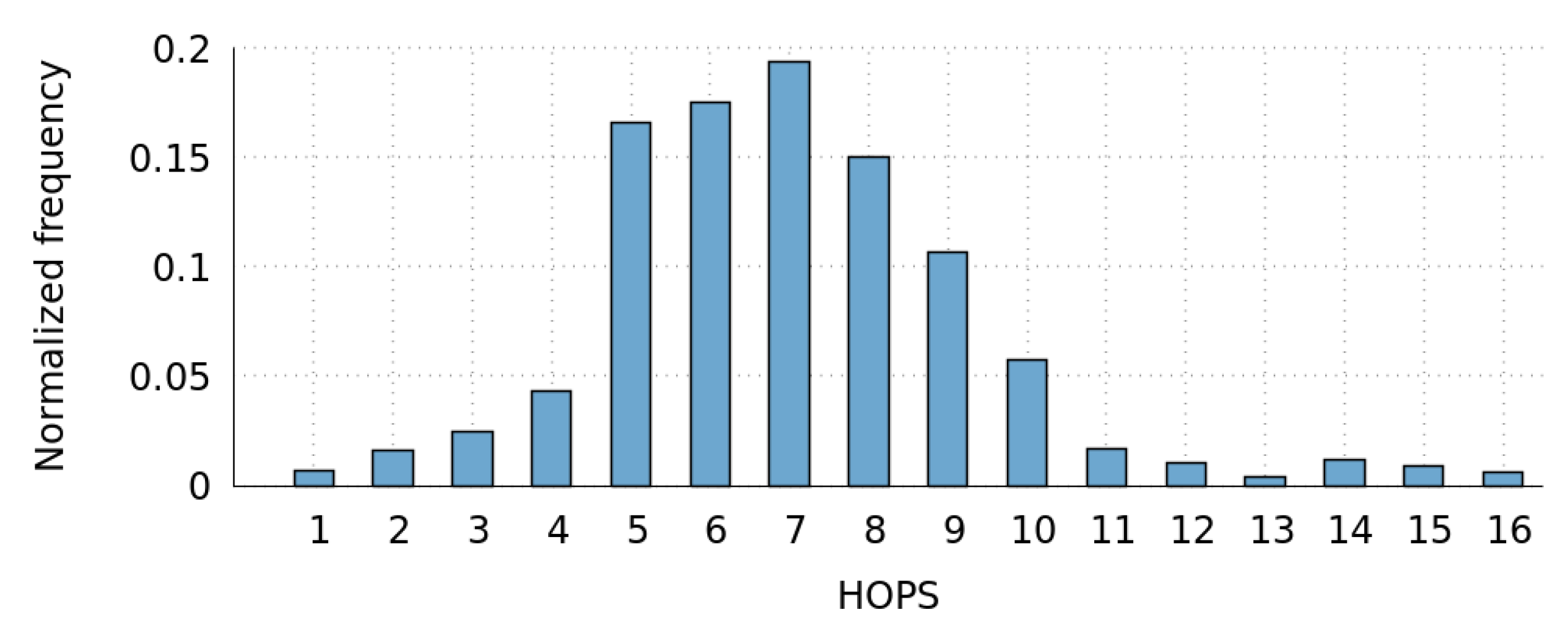
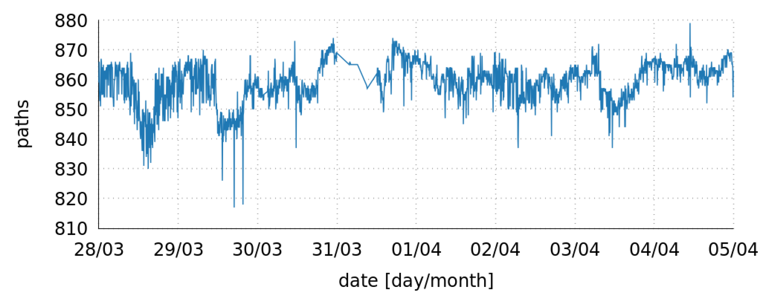
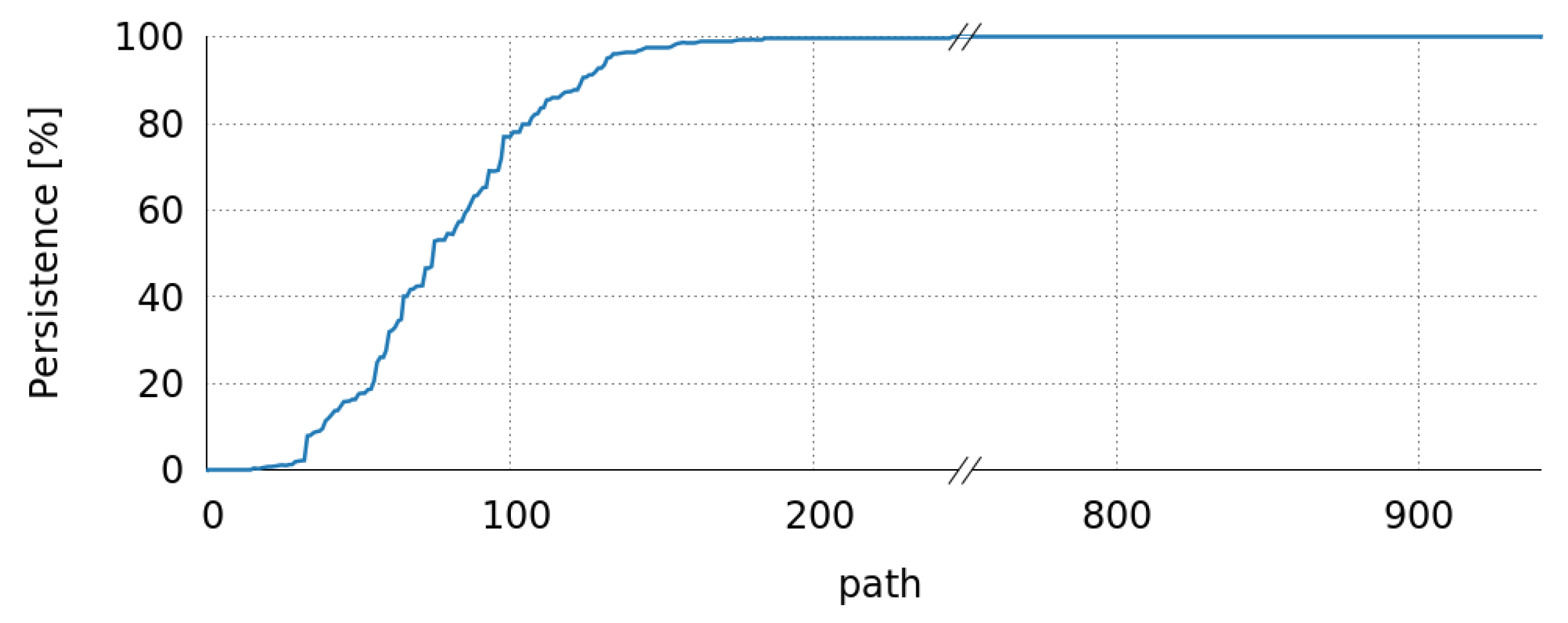
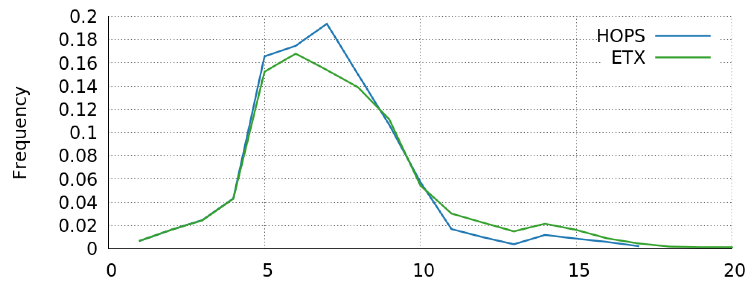
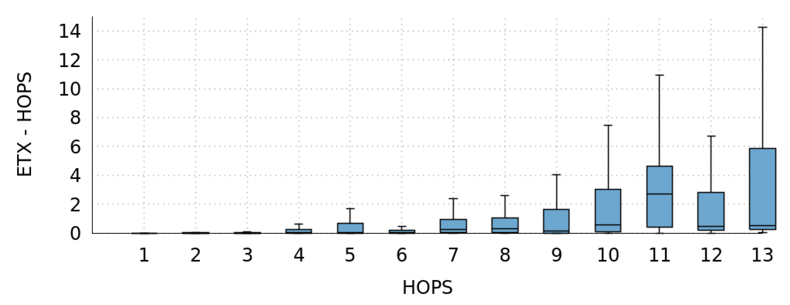
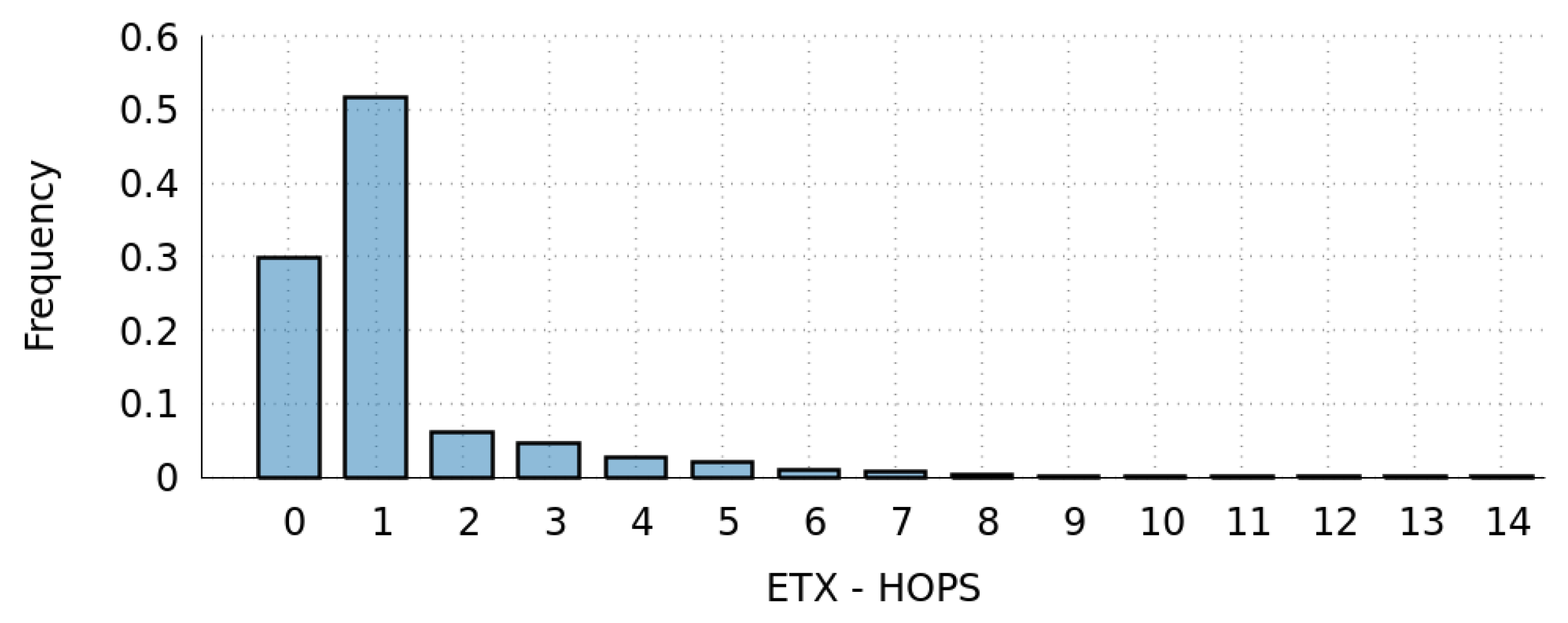
3.2.1. Path Behavior

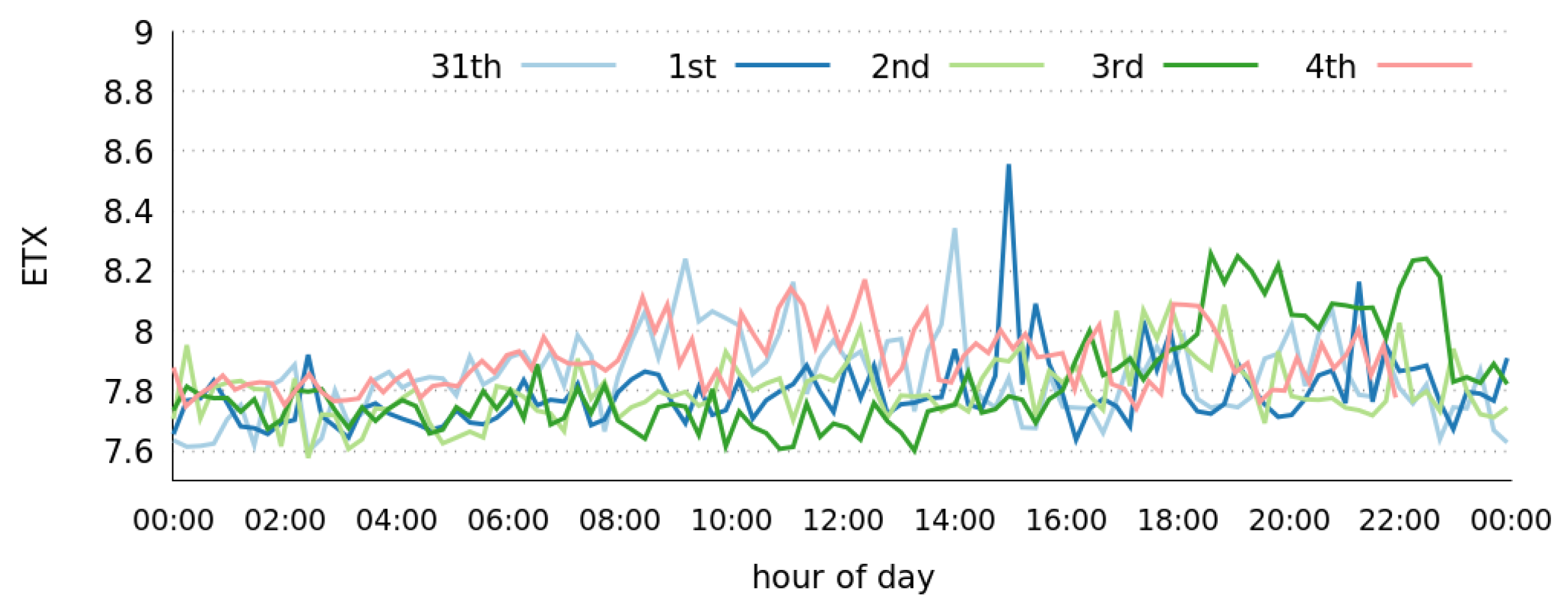
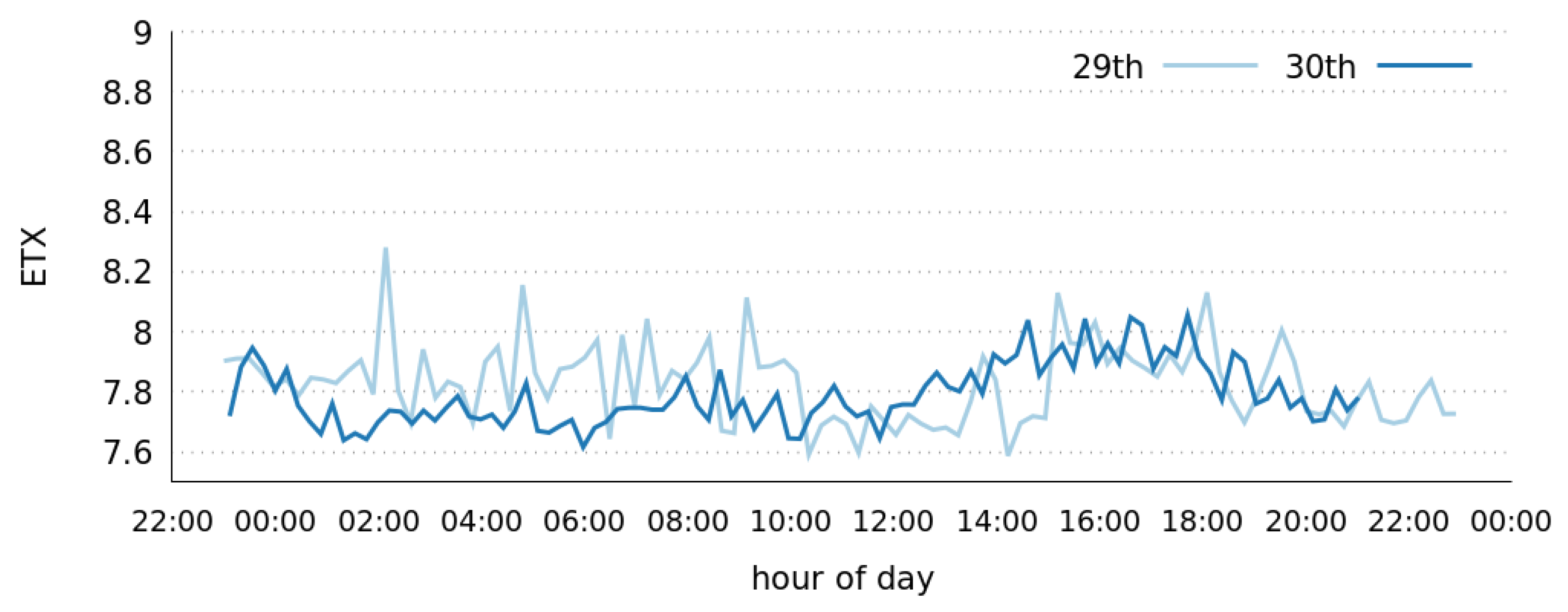
Our first study analyzed the temporal evolution of the number of paths (routing entries). As stated before, Figure 2 shows this evolution during a period of eight days. At any instant of time, each source node can see only one path (the one with best quality) for each possible destination node in the network. We can observe that the fluctuation of the number of paths seen by one node is quite significant (about 7% of variation). This observation contrasts with the general assumption in mesh networks that the number of paths is stable. Multi-Point Relay selection, which is usually made by consensus, does not take into account this observed variation and, therefore, the accuracy of finding the best routes can be compromised. Our time-series-based analysis will consider this variation to make accurate predictions of future EtEQ.

Figure 3 plots the fraction of snapshots over the total for which the path has been present, namely the Persistence of each path. Considering that the snapshots were taken every 5 min, we observed that about 100 paths lie below 80% of persistence, but the remaining 840 paths are very persistent. We noticed that this small number of non-persistent paths can explain the variations in Figure 2. Although the amount of non-persistent paths is significant, a path with very low persistence cannot be useful for predicting the behavior of stable paths. Therefore, taking into account that the dataset represents eight days, for the analysis presented in the following sections, we ignored paths that are persistent fewer than two days in total (persistence below 25%). There are only 57 paths with less than 25% persistence, and the remaining 882 paths have more than 25% persistence. Figure 3 shows that most of these former paths have a great persistence (839 paths have more than 80% persistence).

3.2.2. ETX Behavior

To understand the behavior of ETX Path Quality, we made some additional measurements. Notice that, in the dataset introduced above, the corresponding EtEQ is ETX Path Quality.

Figure 4 shows the evolution of average ETX Path Quality throughout a day, for the five working days included in the dataset. In this figure, it can be seen that average ETX path values are more stable at night, between 00:00 and 08:00. Throughout the day, between 09:00 and 01:00, there are more fluctuations, reaching differences of even 1 ETX. Variation of actual ETX path values can be significantly higher, but this information is hidden by the average value. For non-working days (Figure 5), this behavior is less apparent: the fluctuations and stable periods of working days are no longer seen. Similar patterns are often found in network usage datasets, therefore we can assume that the reasons for the depicted behavior is the variation of network traffic and interference during the day, leading to packet loss. This observation suggests that we possibly have to expect different prediction accuracy depending on the day and time when prediction is applied.

To analyze the relationship between path Hop-count and its corresponding average ETX, Figure 6 plots the frequency of each of these values. We can observe that Hops count and average ETX overlap are between the values of 1 and 4. That means that the quality of short paths is maximum. However, for values 5 or higher, average ETX path values present deviations that can be translated as decreased EtEQ and a large number of needed packet retransmissions needed. Notice that the more frequent values of Hops count and average ETX (more than 10% each) are in the range of 5–9.

In our last study, we analyzed the dispersion of ETX according to the number of Hops. In this way, Figure 7 contains the box plots of the deviation between average ETX and hops. The values were normalized with the corresponding number of hops to provide a better idea of the scale of the deviation, taking into account that the average ETX deviation is not correlated with the number of hops. We can see that the average ETX deviation is minimal for 1–4 Hops, it is significant for 5–9 hops, and relevant for 10–13 hops. We did not consider paths with 14 or more hops because they are very odd cases and are not representative to show the correlation between ETX and hops. Most of them are paths that contain a sequence of nodes connected in a line with fiber. Therefore, we can conclude that the prediction would be more or less accurate depending on the number of Hops.

From the above preliminary observations and dataset studies, we reached the conclusions that from a node’s ego-network point-of-view there is a non-negligible amount of unstable paths for which the average ETX path value shows a significant deviation from the optimal value. To better clarify this issue, Figure 8 provides a histogram of deviation between average ETX and number of hops. Notice that paths with ETX-HOPS of zero are optimal in terms of the routing metric. In this case, just 30% of all paths are included in this category. Moreover, the number of paths (up to 50%) that presents ETX-HOPS within the range [0,1] is quite significant. Finally, 20% of the remaining paths are distributed in the remaining ranges.

In summary, to investigate the EtEQ behavior as well as to find efficient EtEQ prediction strategies based on time-series analysis would result in valuable information for routing in WMCNs.

4. Time-Series Analysis to Predict EtEQ

4.1. Experimental Framework

As stated before, we dealt with time-series analysis to estimate LQ in the routing layer for real-world WMCNs. In this way, the value of the ETX EtEQ prediction of a path can be used as a selection metric by the routing algorithm. OLSR uses the aggregated ETX of each path, selecting the lowest aggregated ETX value. This aggregate value is computed using the measured ETX values in all the links and propagated to the rest of the network. In the case of large networks, this propagation takes a considerable time. As shown in Figure 1, the full propagation could take up to 80 s. In addition, the ETX value of a link is computed based on an active proving history. Therefore, the ETX of a link takes time to show that a link is overloaded. With the ETX EtEQ prediction, we are estimating future values. In this way, the routing algorithm could react to changes in the network, e.g., an overloaded link. To do this, we assume the FunkFeuer experimental network and an OLSR dataset of several nodes and links.

A time series is a set of data collected over time with a natural temporal ordering. It differs from typical Data Mining or Machine Learning applications, where the ordering of data points within a dataset is not important. Time-series analysis is the process of using statistical techniques to model and explain a time-dependent series of data points. Similarly, time-series forecasting is a method that uses a model to generate predictions (forecasts) of future events based on known past events. In our case, we used more than one prediction algorithm, so that we do not rely on a specific learning technique. We applied four of the best well-known approaches [51]: Support Vector Machines (SVM), k-Nearest Neighbors (kNN), Regression Trees (RT), and Rule-Based Regression (RBR).

• The Support Vector Machine (SVM) algorithm has recently become one of the most popular and widely used methods in Machine Learning. It performs a linear or nonlinear division of the input space, and builds a prediction model that assigns target values into one or another category.
• The k-Nearest Neighbors (kNN) algorithm is one of the most simple Machine Learning algorithms as it makes no assumptions on the underlying data distribution. This algorithm takes the k data-points closest to the target value, and picks the most common one.
• Regression Tree (RT) is a type of decision-tree algorithm where the target value can have continuous values. This method recursively partitions the data space and runs a simple prediction model within each partition.
• Finally, the Rule-Based Regression (RBR) algorithm is similar to a decision-tree approach, but it is a stronger model that provides rules that are often potentially more predictive.

We applied training and test-sets validation to assess the predictive accuracy of the models. After a model is processed using the training set, it is tested by making predictions against the test set. Although the algorithms need some days to start making predictions after the appearance of a new path, this work assumes scenarios where nodes and links do not appear very often, as shown in Figure 2. In any case, when there is no room for prediction, the actual ETX is assumed. For this purpose, we used the Weka-workbench system [52], a framework that incorporates a variety of learning algorithms, and some tools for the evaluation and comparison of the results. Weka has a dedicated environment for time-series analysis that allows forecasting models to be developed and evaluated. The Weka’s time-series framework takes a Machine Learning or Data Mining approach to model time-series by transforming the data into a form that can be processed by standard propositional learning algorithms. To do so, it removes the temporal ordering of individual inputs, by encoding the time dependency via additional input fields. More details about the tools and algorithms assumed in this study can be found in

Table 1. Experimental tools and details.

Tools	Version
Weka	version 3.7.10
TimeseriesForecasting	version 1.1.25
Algorithm	Class
RT	weka.classifiers.trees.M5P
RBR	weka.classifiers.rules.M5Rules
kNN	weka.classifiers.lazy.IBk
SVM	weka.classifiers.functions.SMOreg
Algorithm	Parameters
RT	-M 4.0
RBR	-M 4.0
kNN	-K 1 -W 0 -A “weka.core.EuclideanDistance -R first-last”
SVM	-I “weka.classifiers.functions.supportVector.RegSMOImproved -L 0.001 > -W 1 -P 1.0E-12 -T 0.001 -V” -K “weka.classifiers.functions.supportVector.PolyKernel -C 250007 -E 1.0” -N 0

.

Usually, classification studies assess the predictive power of their model by using Mean Absolute Error (MAE) or Root Mean Squared Error (RMSE), both widely used in related work. We considered MAE in our experiments, as it is a common method to evaluate the performance of prediction approaches and gives the same weight to all individual differences. This metric is computed through the following formula: $MAE=sum\left(abs\right(predicted-actual\left)\right)/N$.

Finally, we assumed a lag window size of 12 in all simulations. This value was set based on the analysis of the impact of lag window size performed in [48] that predicts next link quality values in the routing layer of large-scale, distributed and decentralized systems also by means of time series analysis.

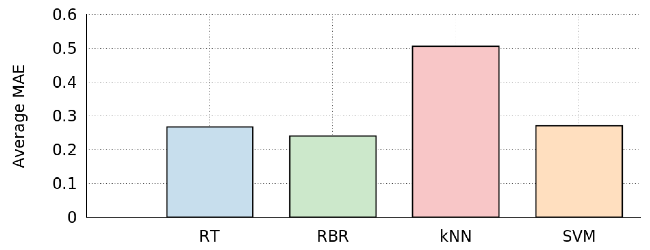
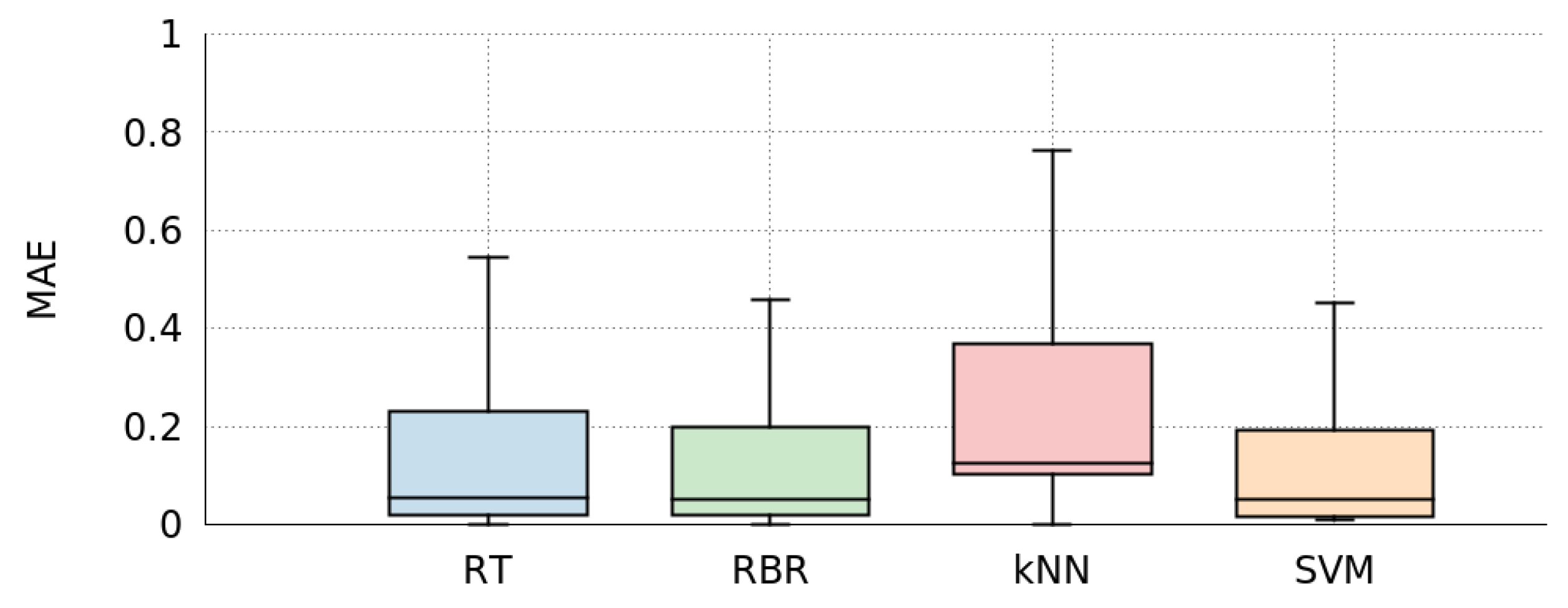
4.2. Comparison of Learning Algorithms Based on Time Series

As stated before, we explored whether time-series analysis can be used to predict future End-to-End Quality (EtEQ) values. To do this, we applied four well-known approaches: SVM, kNN, RT, and RBR.

Figure 9 shows the average Mean Absolute Error (MAE) per path using a training dataset of 2016 instances (seven days), a test dataset of 288 instances (one day), and a lag window composed of the last 12 instances. This test was performed to verify whether time-series learning-algorithms could predict consecutive EtEQ values. These results show that we achieved the best accuracy for the Rule-Based Regression (RBR), and the worst for k-Nearest Neighbors (kNN). Regression Trees (RT) and Support Vector Machines (SVM) also moves very close to RBR results. Notice that the maximum EtEQ value is 1 and, therefore, the MAE per link is 0.24 for RBR and 0.5 for kNN. We applied a T-test to mean values for independent samples (at 95% confidence level) in order to compare the classification algorithms using the MAE. After this analysis, p-values smaller than 0.05 indicate that the means are significantly different, and, therefore, we would reject the null hypothesis of no difference between the means. Consequently, we can claim that time-series analysis achieves high percentages of success, and that among them, RBR seems to be the best candidate to make predictions.

We also analyzed the error variability of each algorithm and represented the results using box plots. Three of the four algorithms achieved similar performance for most of the links (RT, RBR, and SVM), as shown in Figure 10. Although, RT might present some outliers, the differences among median, first quartile, and third quartile are minimal. On the other side, kNN presented different behavior compared to the others. In this case, outliers presented larger errors that increase the average values and change the overall evaluation of the algorithm. In the rest of the paper, we consider the RBR algorithm to show the potential benefits of predicting EtEQ by means of a time-series analysis.

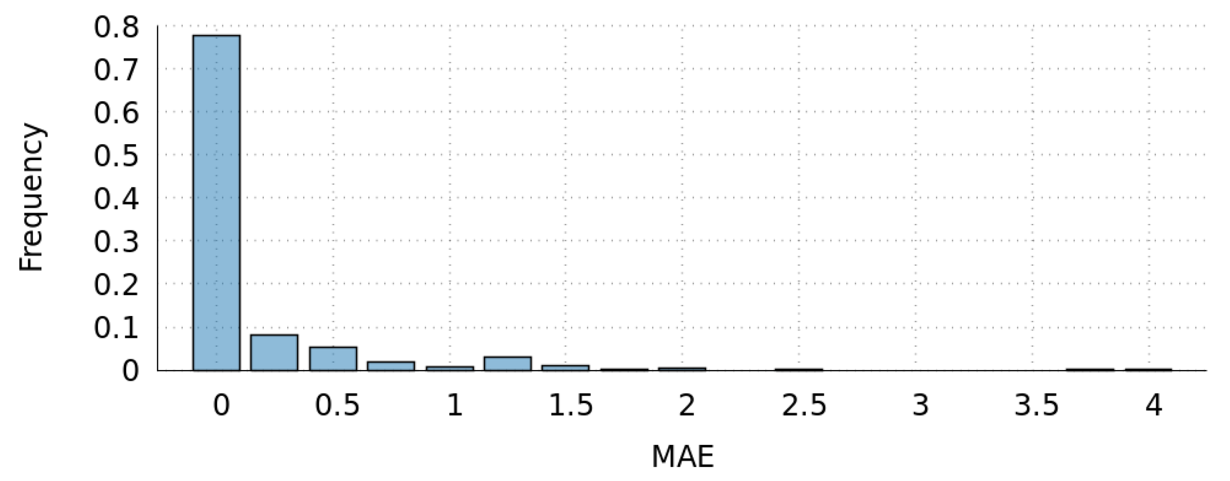
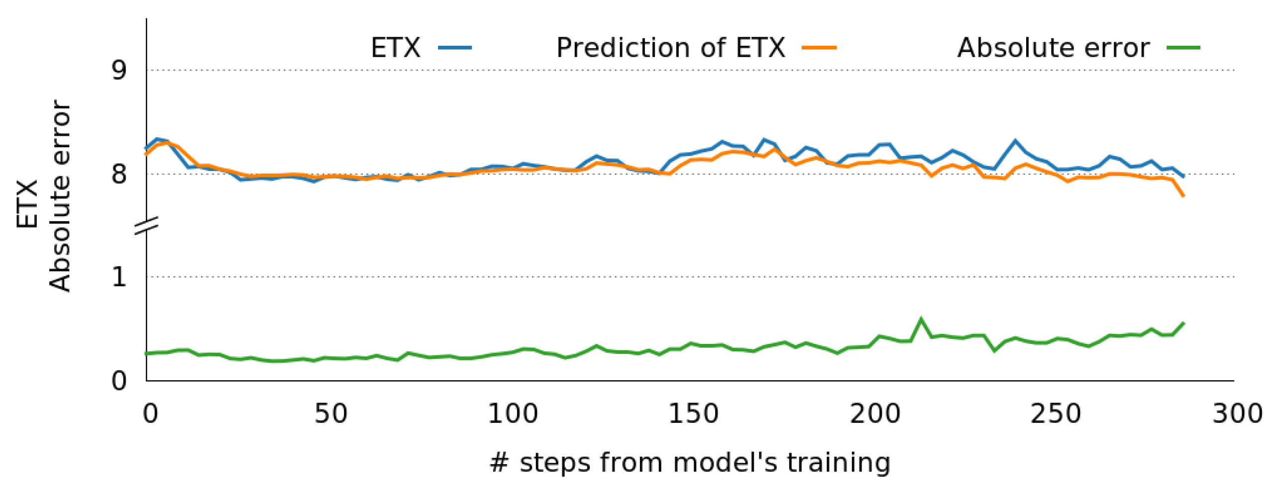
4.3. EtEQ Prediction with Rule-Based Regression

We proceeded next to analyze more in depth the EtEQ using the RBR algorithm to discover how can we reach a satisfactory level of one-step prediction.

Figure 11 presents box plots of the MAE of path ETX prediction with RBR, versus the number of Hops corresponding to the paths. We used the same training dataset as Section 4.2. Even though the dispersion of the error seems high in specific cases (for example 10, 11, and 13 hops), the results follow the dispersion pattern of actual ETX values as described in Figure 7, although at a much smaller scale. In other words, even though ETX values for 10, 11, and 13 hop paths have a high dispersion, our prediction manages to successfully predict a big percentage of the fluctuations. For instance, the dispersion of 13 hop path-ETX is 6, while the error of its prediction has a maximum value of 3.

Figure 12 presents another point of view of the RBR Mean Absolute Error (MAE) to clarify how the mean quality of the path influences the performance of the algorithm. This histogram shows that more than 90% of predictions has a MAE lower than 0.5, almost without error. Moreover, this corresponds to paths with a few hops. The remaining 10%, which presents bigger errors, are associated to paths with many hops (as can be seen in Figure 11).

Figure 13 provides a more detailed analysis of the prediction accuracy. We can see that the average ETX value and the average prediction value are very close, even overlapping during the first half of prediction test. A better estimation for the deviation of the individual path values is given by the average absolute-error line. Notice that the deviation remains less than 0.5 throughout the whole prediction, which is a great achievement. Nevertheless, the potential impact of this small error in routing decisions can be further studied.

Another characteristic of the prediction revealed by Figure 13 is that after 100 steps of prediction (between 08:00 and 08:30) the absolute error presents an increasing trend. We assume that this outcome is an effect of the actual ETX oscillations depicted in Figure 4. To verify this assumption, we performed two more prediction tests. From 00:00 to 12:00 (Figure 14.top) and from 12:00 to 00:00 (Figure 14.bottom), using as training dataset the 2160 more recent instances (7.5 days before prediction starts), a test dataset of 144 instances (half a day), and a lag window composed of the last 12. With these changes in the training configuration (7.5 + 0.5 days), the results obtained are almost identical to the results of Figure 13 (with 7 + 1 days), leading us to conclude that ETX oscillations (higher between 12:00 to 00:00) are indeed influencing the prediction. This led us to consider different predictors for day and night to increase predictor accuracy.

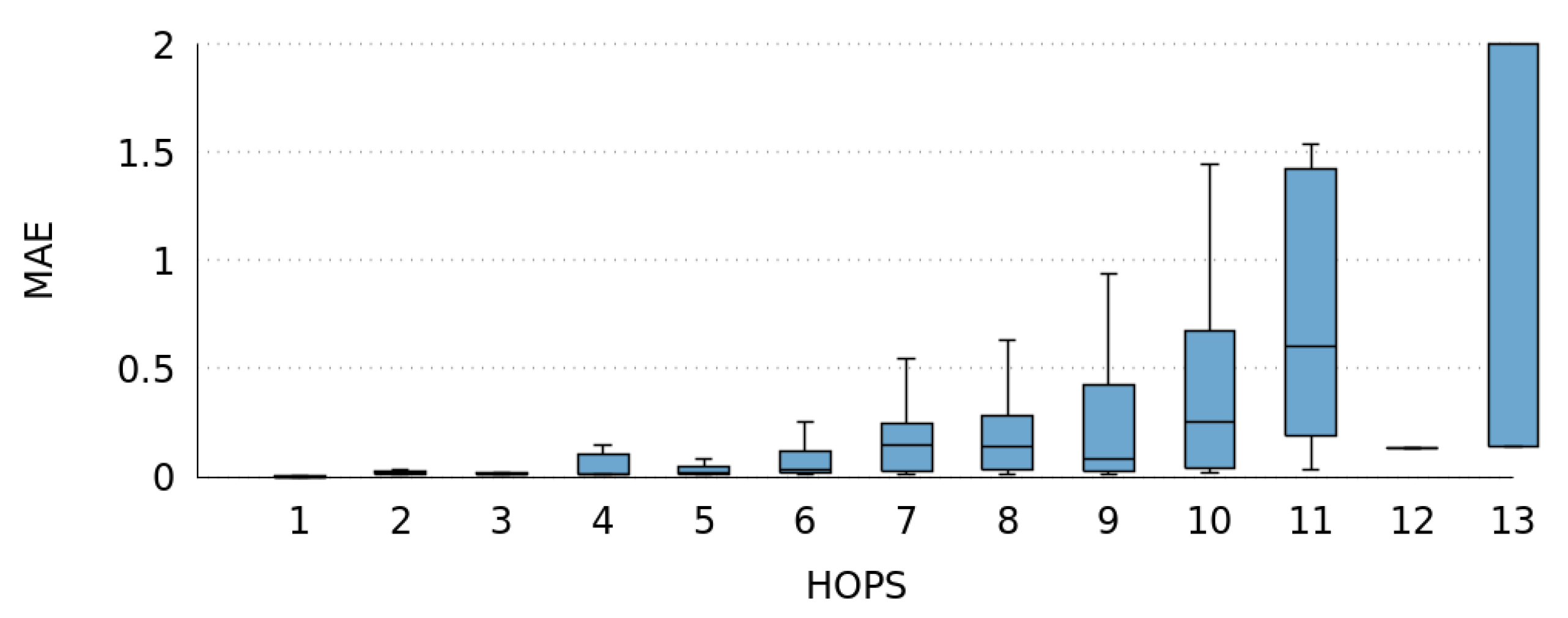
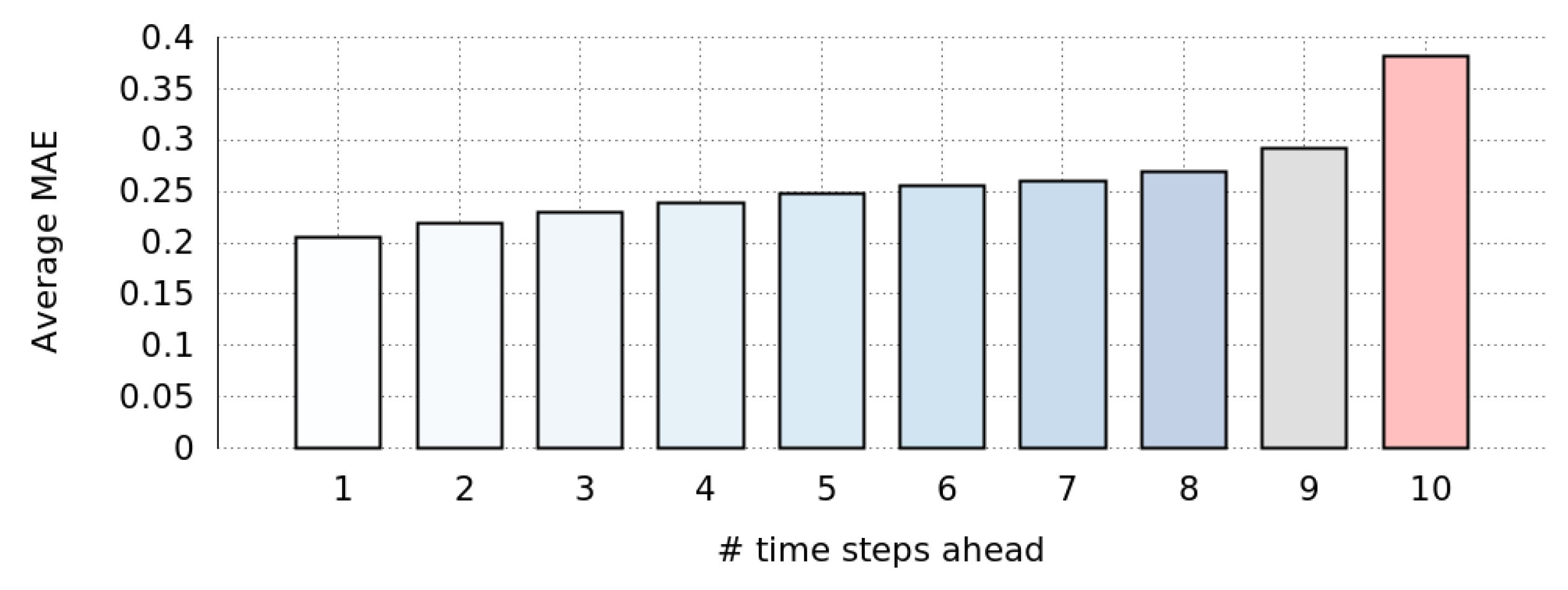
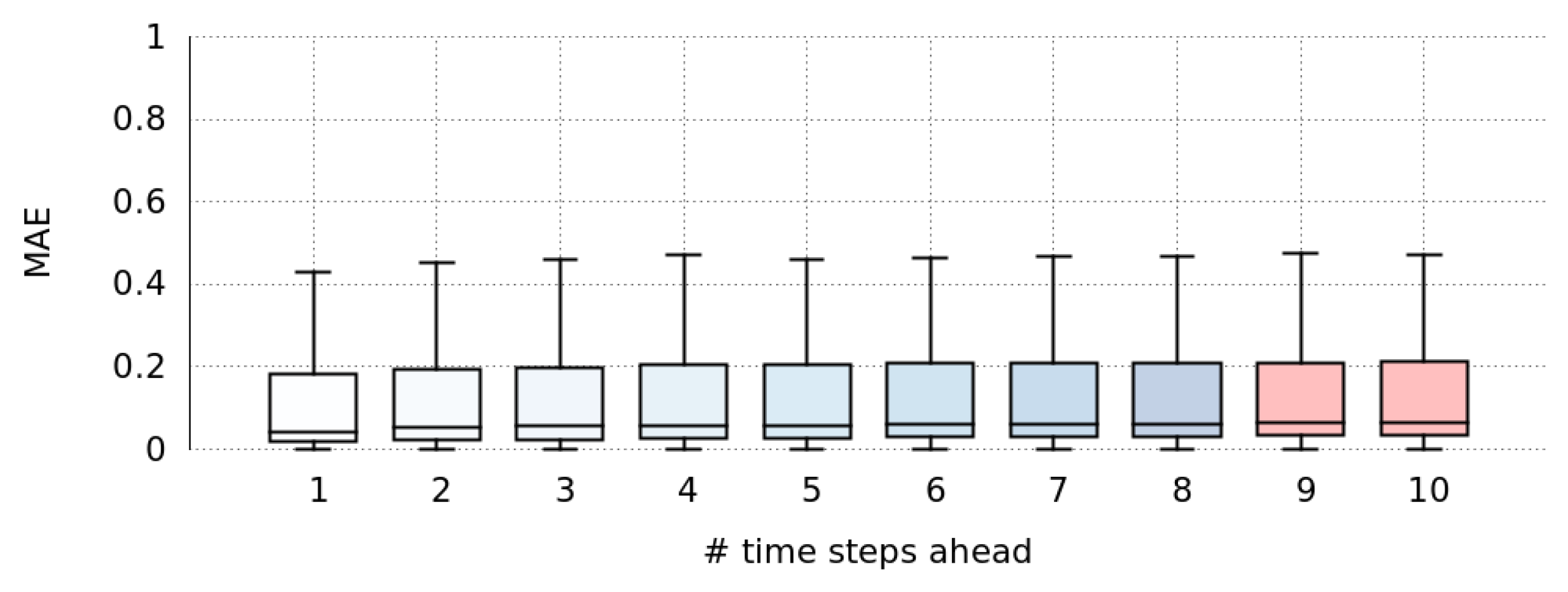
4.4. Prediction of Some Steps Ahead

This analysis was performed to explore if time-series analysis and prediction can be used to predict the value of EtEQ some time-steps ahead into the future.

Figure 15 shows the average MAE of paths. It shows the results of the RBR algorithm using the same setup that the baseline experiment (a lag window size of 12 instances, a training dataset of 2016 instances, and a test dataset of 288 instances), and then predicting 1–10 time steps into the future. The results obtained from the majority of the tests were satisfying. As we can observe, the average MAE grows very slowly. It seems possible to conclude that we could successfully predict the EtEQ several steps ahead in time.

Once more, we analyzed the variability of errors for each number of steps ahead using a box plot, as shown in Figure 16. Although the values for the median and the first quartile are similar for all steps ahead considered, the values of third quartile and outliers (not depicted) grow with the number of steps. These differences in the variability of errors lead to the differences in the average Mean Absolute Error (MAE).

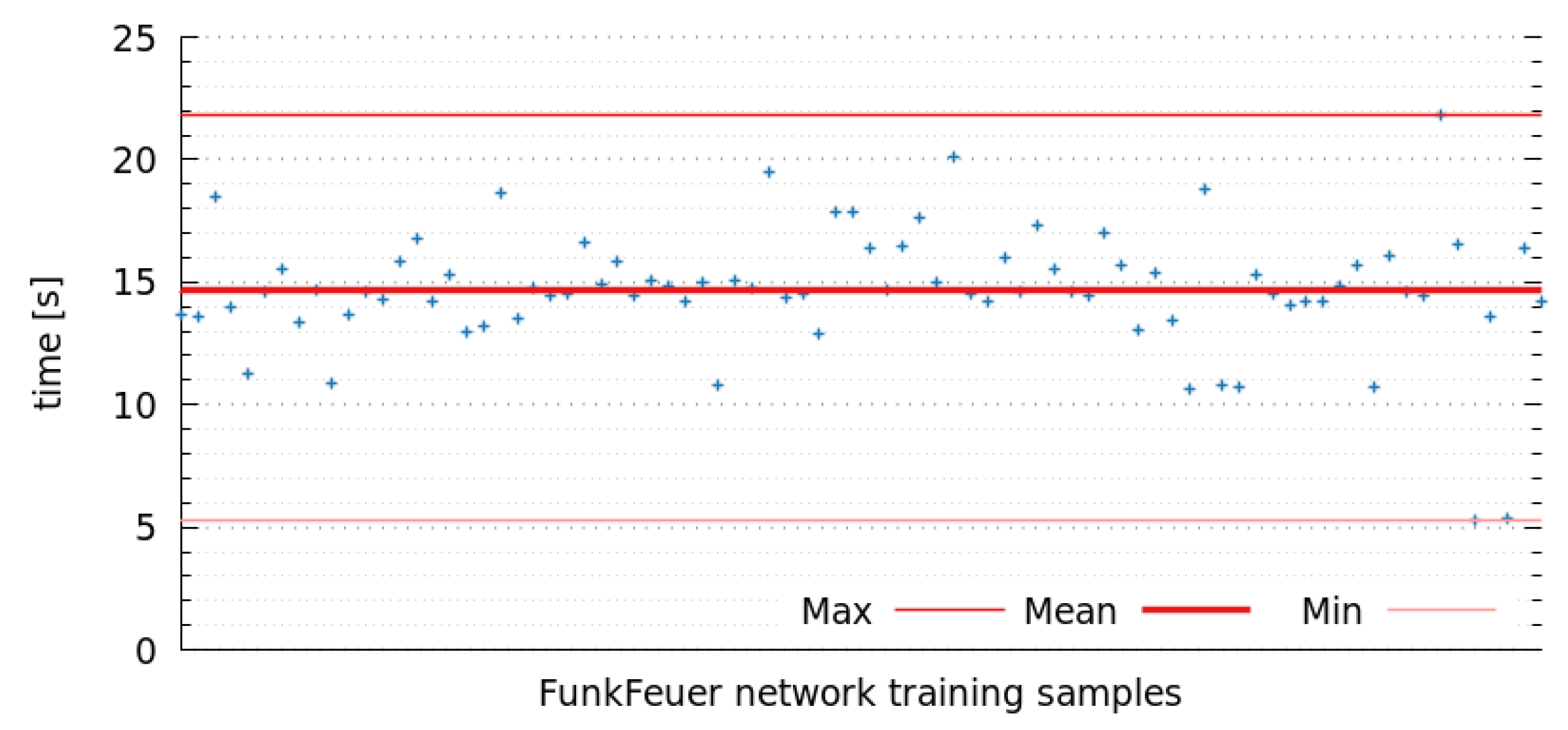
4.5. Computational Cost of the Predictions

We analyzed the computational cost of the training algorithm and the prediction process in a real environment. The aim of this analysis was to verify that this cost is low and does not represent a significant increase in terms of computational resources nor energy. For this purpose, we executed the prediction software in a typical mini-PC, which acts as router, using the WEKA [52] environment with the FunkFeuer network open datasets [6]. The mini-PC is a Jetway JBC372F36W-2600-B [53]. The processor is an Intel ATOM N2600 at 1.6 GHz with two cores and multithread support. It has 4 GB of RAM and a SSD connected to a SATA2 port. The system was configured with a Linux kernel 4.4.0-140 in 64 bit mode inside an Ubuntu 16.04 LTS distribution. To execute the WEKA environment, the Java openjdk version 1.8.0-191 was installed.

We considered three parameters: CPU utilization, energy consumption and temperature. For the first one, we split the measurements into two parts: in one side the cost of the prediction and on the other side the cost of the training. We evaluated the execution assuming the worst case, which means executing the prediction every 5 s and the training every 5 min (in a real scenario, the training frequency should be once every few hours). WEKA environment takes a huge amount of time to wake-up compared to the cost of making a single prediction; that is around 3 s versus a few milliseconds. To isolate the cost of one prediction, we executed multiple times (100–1000) several routing tables from FunkFeuer network open datasets [6] with the statistical model preloaded. Figure 17 shows the difference in time of one prediction obtained from the subtract of just 13 predictions—the minimum possible value—over 14 predictions (one step), and the difference in time from the subtract of just 13 predictions over 23 predictions divided by 10 (ten steps). Then, we estimated the execution time of one prediction once the WEKA environment was started and the model was loaded. We observed a computational cost in the range from 20 ms to 80 ms with a 35 ms on average. This result led us to conclude that computational cost of predictions is negligible.

In the same way, we also executed the training part using WEKA. One execution of the training part allocates both CPUs at 100% for a period of time from 5 to 22 s. Figure 18 shows the execution time of several samples from FunkFeuer network open datasets. We observed that it takes about 15 s on average, which is a substantial amount of time. However, we have to consider that this training is performed every few hours in a real environment, thus the impact in CPU utilization is very low. Moreover, we decided to test an extreme situation, presented in Figure 19, where we executed the training algorithm every 5 min over 24 h to observe that just a 3.78% of CPU is needed to execute the training part of the model.

The second parameter that we evaluated was the energy consumption of the training algorithm. To do this, we attached a voltmeter and an ammeter to the 12 V jack of the mini-PC. This allowed us to measure real volt and amp consumption when the system is in idle state, and when the system is executing the training model at full CPU utilization. Figure 20 shows the energy consumption in watts for a period of 20 min. The system executed training models continuously and sequentially. We observed that the increase is 1.86 W on average, but in a real environment, this only happens for a period of 15 s every few hours. Again, we can conclude that the training algorithm does not substantially increase the energy consumption of the system.

Finally, we also measured the temperature of both cores in the system for a period of 24 h. To do this, we forced the system to assume the worst case, i.e., executing the training algorithm every 5 min. Figure 21 shows that the system reaches a temperature around 40 ${}^{\circ }$C in a normal state, and that it has an increase of close to 5 ${}^{\circ }$C when it is executing the training algorithm. Notice that mean values are close to the idle state because in this scenario the algorithm is only active 5% of the time.

5. Use Case Analysis

5.1. Experimental Framework

In this section, we present simulations that compared under several load conditions the overall network performance between: (a) the proposed EtEQ prediction strategy; and (b) a simplified version of OLSR, i.e., ETX + Dijkstra. Even though both routing strategies are pretty similar, their main difference is that the latter uses directly the real past link quality values, while the former uses predicted values based on past link quality values. Prediction provides us the benefit of making routing decisions earlier, at the expense of assuming values that may be erroneous.

The routing strategies are compared using a simulator that we developed using JavaSim [54], an object-oriented simulation package based on C++SIM, that provides discrete event process-based simulation similar to SIMULA’s simulation class and libraries. The simulations performed followed a setup similar to Fadlullah et al. [21]. We considered the same static scenario: a $4\times 4$ wireless mesh backbone network, where edge routers generate packets for other edge routers, and inner routers only forward packets. The two main differences are that we dealt with time slots and we considered a heterogeneous network (both links and nodes). The network was simulated during 30,000 time slots and a random initial-time (in slots) was assumed to start the packet transmission.

Our simulator was developed assuming a set of routing and link characteristics that can deliver more realistic results. In these simulations, we assumed 2000 previous samples (time slots) to train a model and any new model was trained every 300 time slots. Moreover, we also assumed a lag window size of 12. On the other side, the predictor predicted EtEQ of the next round (one time slot). The ETX of a link, recalculated in real time every single time slot, was computed based on all the messages that were received and not only with the HELLO messages of the routing algorithm. The routing algorithm calculated the routing tables of each node every 100 time slots, and was omniscient in the sense that it knew the ETX of all the links without the need of broadcasted messages. The delay of the links was proportional to the size of the pending messages queue of the node and therefore can be different in any direction.

Considering that in a real network, packet pending queues of the nodes are finite, we needed to model packet dropping caused by packet overload. We considered that 1 packet every 100 slots is a very low overload, 1 packet every 10 slots is an overload close to the maximum of the network and 1 packet every 1 slot is a fully overloaded network. We simulated two different approaches in terms of packet dropping: (1) a fail every ten packets; and (2) a fail every two packets. This parameter is denoted as Mean Time Between Failures (MTBF). Notice that a two-packet MTBF can be considered as an extreme failure-rate.

Moreover, the same scenario of previous sections was assumed to analyze the fault tolerance of packets in the presence of link failures (packet dropping). Therefore, we assumed three different link-failure models: (1) none; (2) uniform; and (3) Pareto. The uniform model followed a uniform distribution that has a constant probability. Unfortunately, this failure model is memoryless, which means that it does not reflect the bursty nature of failures, also known as the long-range dependency. For a more realistic model, we used a self-similar process, such as the Pareto distribution, as a long-tail failure-model.

Once the system was configured in the simulator, the experiments were run under several release-times for the messages in the source nodes (network load). To this end, we tested data-packet generation rates of 1 packet sent every 100, 10 and 1 time slots. Hence, we were able to evaluate the network behavior, and the loads in the links for each path. Particularly, we measured Packet Delivery Ratio (PDR), i.e., ratio of packets successfully received compared to the total sent, End-to-End Delay (EtED), and ETX of links.

5.2. Analysis of Results

To evaluate the impact of the prediction on the network messages, we first studied the Packet Delivery Ratio (PDR).

Table 2. Packet delivery ratio (PDR) under diverse load conditions.

	1 Packet Every 100 Slots	1 Packet Every 10 Slots	1 Packet Every 1 Slots
ETX + Dijkstra	1.0	0.98	0.44
End-to-End Quality Prediction	1.0	0.98	0.54

shows the results obtained simulating diverse network load conditions. We can observe that both EtEQ prediction and ETX + Dijkstra presented a similar delivery rate. When links were not overloaded, the behavior was equal, showing that the few prediction errors did not produce path changes. On the other hand, when links were overloaded due to data traffic, our approach detected earlier this situation. In this last case, EtEQ prediction achieved 22.7% better delivery rates.

We also analyzed the PDR behavior under link failures, as shown in

Table 3. Packet delivery ratio (PDR) with link failures.

	None	Uniform 10	Uniform 2	Pareto 10	Pareto 2
ETX + Dijkstra	1.0	0.99	0.91	1.0	0.89
End-to-End Quality Prediction	1.0	0.98	0.90	1.0	0.89

. Both strategies showed very similar behavior, with differences below 1%, which we considered insignificant. Therefore, we argue that the predictor is not able to foresee link failures.

In our next set of simulations, we measured the quality of links for the compared routing strategies, using ETX of links and EtED. We first studied the ETX, as computed when the network was overloaded. In Figure 22, we can observe the frequency of the diverse ETX values (ETX values close to 1 are better, because they are less overloaded). From the results in this figure, we can argue that, using EtEQ prediction, the average ETX of links is higher, thus the observed link quality is increased. Additionally, the deviation of the quality of the proposed strategy is lower than the one using ETX + Dijkstra, resulting to a better behavior. Finally, when the quality of a link deteriorates, EtEQ prediction allows the routing algorithm to adapt earlier than ETX + Dijkstra. Therefore, we argue that the former reacts earlier upon an overloaded link.

The second metric we used to evaluate both prediction approaches was EtED, where lower values are better. Figure 23 shows the histogram of EtED normalized values. Overall, EtEQ presents similar EtED values to ETX + Dijkstra. Nevertheless, when the network was overloaded, EtEQ values were slightly higher (worse) than ETX + Dijkstra. As observed in the figure, when the quality of a link declines, the EtEQ routing algorithm changes earlier to a new path. This implies an earlier reaction before link overloading. Moreover, under the proposed approach, the new paths used are less overloaded, resulting in an improved Packet Delivery Ratio (PDR, as previously shown in Table 2 and Table 3). On the contrary, the new chosen paths are equal or slightly larger (in HOPS), thus the delivery times are higher (worse). Finally, for the cases of EtEQ prediction failures, i.e., changes in the used path, the new paths are equal or slightly larger (in HOPS), contributing to higher delivery times without achieving a higher PDR.

Our simulations were very small compared to real WMCN such as Funkfeuer network. Therefore, it is difficult to generalize the simulation results to Funkfeuer network. Nevertheless, we believe that dealing with EtEQ prediction may be useful with paths that present the most overloaded links.

6. Conclusions

This study demonstrated that time-series analysis is a promising approach to accurately predict EtEQ values in Community Networks. This technique can be used to improve the performance of the routing protocol, by providing information to make appropriate and timely decisions, to maximize the delivery rate and minimize traffic congestion.

The dataset that we used in our analysis shows quite significant fluctuations (about 7%) in the temporal evolution of the number of paths (routing entries). This contrasts with the general assumption in mesh networks that the number of paths is stable. The persistence of paths in our dataset is very stable for 90% of paths, but 10% of paths have persistence values below 60%, and those paths create the temporal fluctuations in the number of paths. Our study includes paths with persistence above 25%.

Regarding the Expected Transmission Count (ETX) behavior, the average ETX Path Quality is more stable at night, and presents more fluctuations during the morning. On non-working days, this behavior is less apparent. We assume this is caused by the variation of network traffic and interference during the day, leading to packet loss. Hence, the accuracy of prediction depends on the day and time when it is applied.

On the other side, the most frequent number of Hops and ETX values are in the range of 5–10. The dispersion of ETX according to the number of Hops is minimal for 1–4 Hops and more than 14 Hops. However, the dispersion is significant for 5–9 Hops, and relevant for 10–13 Hops. Therefore, the accuracy of the predictions would be better or worse depending on the number of Hops.

We present results from four well known learning algorithms that model time series: Support Vector Machine (SVM), k-Nearest Neighbors (kNN), Regression Tree (RT), and Rule-Based Regression (RBR). All of them achieved high percentages of success, with average Mean Absolute Error values per link between 2.4% and 5% when predicting the next value of the EtEQ.

We also analyzed the error variability and found that three of the learning algorithms presented similar performance (RT, RBR, and SVM), whereas kNN performed worse due to outliers with larger errors. A more detailed study of RBR prediction showed an average absolute-error less than 1. We also observed differences in the prediction behavior during day and during night, as happened with actual ETX values.

Additionally, we also measured the computational cost of the prediction concluding that the proposed methodology does not consume significant amount of resources and that the impact in a router system is very low in terms of CPU utilization, energy consumption and temperature.

Finally, the analysis of a use case allowed us to compare two routing strategies. The results show that our approach behaved equal to or better than ETX + Dijkstra in terms of Packet Delivery Ratio and Link ETX. However, the End-to-End Delay metric presented slightly worse results.

As future work, we want to extend this analysis to other Community Networks [8] to evaluate if the observed behavior could be generalized. Moreover, we plan to identify which Paths contribute most to the error in the EtEQ prediction and to understand what factors make it more difficult to predict the behavior of these paths. We also want to study the impact of errors in routing decisions, and to explore how accuracy could be increased by deploying two different predictors, for day and night. Finally, we plan to improve the prediction process by discarding those paths whose relation between EtEQ and prediction accuracy is above a certain threshold. This discarding can be done at the very beginning (static discarding) or at any given time (dynamic discarding).

References

1. United Nations Internet Governance Forum. Community Networks: The Internet by the People, for the People. Official Outcome of the UN IGF Dynamic Coalition on Community Connectivity. 2017. Available online: http://hdl.handle.net/10438/19401 (accessed on 17 December 2018).
2. Internet Society. Community Networks. 2018. Available online: https://www.internetsociety.org/issues/community-networks/ (accessed on 17 December 2018).
3. Association for Progressive Communications (APC). APC Communiqué: Employment and Funding Opportunities for Strengthening Community Networks and Local Access. 2018. Available online: https://www.apc.org/en/news/apc-communique-employment-and-funding-opportunities-strengthening-community-networks-and-local (accessed on 17 December 2018).
4. Avonts, J.; Braem, B.; Blondia, C. A questionnaire based examination of community networks. In Proceedings of the 2013 IEEE 9th International Conference on Wireless and Mobile Computing, Networking and Communications (WiMob), Lyon, France, 7–9 October 2013; pp. 8–15. [Google Scholar] [CrossRef]
5. Vega, D.; Baig, R.; Cerdà-Alabern, L.; Medina, E.; Meseguer, R.; Navarro, L. A technological overview of the guifi.net community network. Comput. Netw. 2015, 93, 260–278. [Google Scholar] [CrossRef] [Green Version]
6. FunkFeuer Wien. FunkFeuer, a Free, Experimental Network in Vienna. 2003. Available online: https://www.funkfeuer.at/ (accessed on 19 February 2017).
7. AWMN. Athens Wireless Metropolitan Network. 2010. Available online: http://www.awmn.net/ (accessed on 23 February 2018).
8. Baig, R.; Roca, R.; Freitag, F.; Navarro, L. Guifi.net, a crowdsourced network infrastructure held in common. Comput. Netw. 2015, 90, 150–165. [Google Scholar] [CrossRef]
9. Braem, B.; Blondia, C.; Barz, C.; Rogge, H.; Freitag, F.; Navarro, L.; Bonicioli, J.; Papathanasiou, S.; Escrich, P.; Baig Viñas, R.; et al. A Case for Research with and on Community Networks. SIGCOMM Comput. Commun. Rev. 2013, 43, 68–73. [Google Scholar] [CrossRef]
10. Woo, A.; Tong, T.; Culler, D. Taming the Underlying Challenges of Reliable Multihop Routing in Sensor Networks. In Proceedings of the 1st international Conference on Embedded Networked Sensor Systems (SenSys), Los Angeles, CA, USA, 5–7 November 2003; pp. 14–27. [Google Scholar] [CrossRef]
11. Draves, R.; Padhye, J.; Zill, B. Comparison of Routing Metrics for Static Multi-hop Wireless Networks. SIGCOMM Comput. Commun. Rev. 2004, 34, 133–144. [Google Scholar] [CrossRef]
12. Koksal, C.E.; Balakrishnan, H. Quality-Aware Routing Metrics for Time-Varying Wireless Mesh Networks. IEEE J. Sel. Areas Commun. 2006, 24, 1984–1994. [Google Scholar] [CrossRef]
13. Rault, T.; Bouabdallah, A.; Challal, Y. Energy efficiency in wireless sensor networks: A top-down survey. Comput. Netw. 2014, 67, 104–122. [Google Scholar] [CrossRef]
14. Rodríguez-Covili, J.; Ochoa, S.F.; Pino, J.A.; Messeguer, R.; Medina, E.; Royo, D. A communication infrastructure to ease the development of mobile collaborative applications. J. Netw. Comput. Appl. 2011, 34, 1883–1893. [Google Scholar] [CrossRef]
15. Vural, S.; Wei, D.; Moessner, K. Survey of Experimental Evaluation Studies for Wireless Mesh Network Deployments in Urban Areas Towards Ubiquitous Internet. IEEE Commun. Surv. Tutor. 2013, 15, 223–239. [Google Scholar] [CrossRef]
16. Baccour, N.; Koubâa, A.; Mottola, L.; Zúñiga, M.A.; Youssef, H.; Boano, C.A.; Alves, M. Radio Link Quality Estimation in Wireless Sensor Networks: A Survey. ACM Trans. Sens. Netw. 2012, 8, 34:1–34:33. [Google Scholar] [CrossRef]
17. Lü, L.; Zhou, T. Link prediction in complex networks: A survey. Phys. A Stat. Mech. Its Appl. 2011, 390, 1150–1170. [Google Scholar] [CrossRef] [Green Version]
18. Trammell, B.; Smith, J.; Perrig, A. Adding Path Awareness to the Internet Architecture. IEEE Internet Comput. 2018, 22, 96–102. [Google Scholar] [CrossRef]
19. Millan, P.; Molina, C.; Dimogerontakis, E.; Navarro, L.; Meseguer, R.; Braem, B.; Blondia, C. Tracking and Predicting End-to-End Quality in Wireless Community Networks. In Proceedings of the 2015 3rd International Conference on Future Internet of Things and Cloud (FiCloud), Rome, Italy, 24–26 August 2015; pp. 794–799. [Google Scholar] [CrossRef]
20. Millan, P.; Molina, C.; Medina, E.; Vega, D.; Meseguer, R.; Braem, B.; Blondia, C. Tracking and Predicting Link Quality in Wireless Community Networks. In Proceedings of the 2014 IEEE 10th International Conference on Wireless and Mobile Computing, Networking and Communications (WiMob), Larnaca, Cyprus, 8–10 October 2014; pp. 239–244. [Google Scholar] [CrossRef]
21. Fadlullah, Z.M.; Tang, F.; Mao, B.; Kato, N.; Akashi, O.; Inoue, T.; Mizutani, K. State-of-the-art deep learning: Evolving machine intelligence toward tomorrow’s intelligent network traffic control systems. IEEE Commun. Surv. Tutor. 2017, 19, 2432–2455. [Google Scholar] [CrossRef]
22. Xie, J.; Yu, F.R.; Huang, T.; Xie, R.; Liu, J.; Liu, Y. A survey of machine learning techniques applied to software defined networking (SDN): Research issues and challenges. IEEE Commun. Surv. Tutor. 2018, 21, 393–430. [Google Scholar] [CrossRef]
23. Bote-Lorenzo, M.L.; Gómez-Sánchez, E.; Mediavilla-Pastor, C.; Asensio-Pérez, J.I. Online machine learning algorithms to predict link quality in community wireless mesh networks. Comput. Netw. 2018, 132, 68–80. [Google Scholar] [CrossRef] [Green Version]
24. Meseguer, R.; Molina, C.; Ochoa, S.F.; Santos, R. Energy-Aware Topology Control Strategy for Human-Centric Wireless Sensor Networks. Sensors 2014, 14, 2619–2643. [Google Scholar] [CrossRef] [PubMed] [Green Version]
25. Meseguer, R.; Molina, C.; Ochoa, S.F.; Santos, R. Reducing energy consumption in human-centric wireless sensor networks. In Proceedings of the IEEE Conference on Systems, Man, and Cybernetics (SMC), Seoul, Korea, 14–17 October 2012; pp. 1473–1478. [Google Scholar] [CrossRef]
26. Härri, J.; Filali, F.; Bonnet, C. Kinetic Multipoint Relaying: Improvements Using Mobility Predictions. In IFIP International Working Conference on Active and Programmable Networks; Springer: Berlin/Heidelberg, Germany, 2009; pp. 224–229. [Google Scholar] [CrossRef]
27. Maleki, M.; Dantu, K.; Pedram, M. Lifetime prediction routing in mobile ad hoc networks. In Proceedings of the 2003 IEEE Wireless Communications and Networking, New Orleans, LA, USA, 16–20 March 2003; Volume 2, pp. 1185–1190. [Google Scholar] [CrossRef]
28. Kim, D.; Garcia-Luna-Aceves, J.J.; Obraczka, K.; Cano, J.C.; Manzoni, P. Routing mechanisms for mobile ad hoc networks based on the energy drain rate. IEEE Trans. Mob. Comput. 2003, 2, 161–173. [Google Scholar] [CrossRef] [Green Version]
29. Luo, Y.; Wang, J.; Chen, S. An energy-efficient DSR routing protocol based on mobility prediction. In Proceedings of the Symposium on a World of Wireless, Mobile and Multimedia Networks (WoWMoM), Buffalo, NY, USA, 26–29 June 2006. [Google Scholar] [CrossRef]
30. Fonseca, R.; Gnawali, O.; Jamieson, K.; Levis, P. Four-Bit Wireless Link Estimation. In Proceedings of the ACM Workshop on Hot Topics in Networks (HotNets), Atlanta, GA, USA, 14–15 November 2007. [Google Scholar]
31. Ma, Y. Improving wireless link delivery ratio classification with packet SNR. In Proceedings of the 2005 IEEE International Conference on Electro Information Technology, Lincoln, NE, USA, 22–25 May 2005; p. 6. [Google Scholar] [CrossRef]
32. Senel, M.; Chintalapudi, K.; Lal, D.; Keshavarzian, A.; Coyle, E.J. A Kalman Filter Based Link Quality Estimation Scheme for Wireless Sensor Networks. In Proceedings of the IEEE Global Telecommunications Conference (GLOBECOM), Washington, DC, USA, 26–30 November 2007; pp. 875–880. [Google Scholar] [CrossRef]
33. Cerpa, A.; Wong, J.L.; Potkonjak, M.; Estrin, D. Temporal Properties of Low Power Wireless Links: Modeling and Implications on Multi-hop Routing. In Proceedings of the Symposium on Mobile Ad Hoc Networking and Computing (MobiHoc), Champaign, IL, USA, 25–27 May 2005; ACM: New York, NY, USA, 2005; pp. 414–425. [Google Scholar] [CrossRef]
34. De Couto, D.S.J.; Aguayo, D.; Bicket, J.; Morris, R. A High-throughput Path Metric for Multi-hop Wireless Routing. In Proceedings of the Conference on Mobile Computing and Networking (MobiCom), San Diego, CA, USA, 14–19 September 2003; ACM: New York, NY, USA, 2003; pp. 134–146. [Google Scholar] [CrossRef]
35. Renner, C.; Ernst, S.; Weyer, C.; Turau, V. Prediction Accuracy of Link-Quality Estimators. In Wireless Sensor Networks; Springer: Berlin/Heidelberg, Germany, 2011; pp. 1–16. [Google Scholar] [Green Version]
36. Passos, D.; Albuquerque, C.V.N. A Joint Approach to Routing Metrics and Rate Adaptation in Wireless Mesh Networks. IEEE/ACM Trans. Netw. 2012, 20, 999–1009. [Google Scholar] [CrossRef]
37. Banerjee, S.; Misra, A. Minimum Energy Paths for Reliable Communication in Multi-hop Wireless Networks. In Proceedings of the Symposium on Mobile Ad Hoc Networking & Computing (MobiHoc), Lausanne, Switzerland, 9–11 June 2002; ACM: New York, NY, USA, 2002; pp. 146–156. [Google Scholar] [CrossRef]
38. Jakllari, G.; Eidenbenz, S.; Hengartner, N.; Krishnamurthy, S.V.; Faloutsos, M. Link Positions Matter: A Noncommutative Routing Metric for Wireless Mesh Network. In Proceedings of the IEEE Conference on Computer Communications (INFOCOM), Rio de Janeiro, Brazil, 29 August 2008; pp. 744–752. [Google Scholar] [CrossRef]
39. Li, H.; Cheng, Y.; Zhou, C.; Zhuang, W. Minimizing End-to-End Delay: A Novel Routing Metric for Multi-Radio Wireless Mesh Networks. In Proceedings of the IEEE Conference on Computer Communications (INFOCOM), Rio de Janeiro, Brazil, 19–25 April 2009; pp. 46–54. [Google Scholar] [CrossRef]
40. Wang, Y.; Martonosi, M.; Peh, L.S. A New Scheme on Link Quality Prediction and Its Applications to Metric-based Routing. In Proceedings of the Conference on Embedded Networked Sensor Systems (SenSys), San Diego, CA, USA, 2–4 November 2005; pp. 288–289. [Google Scholar] [CrossRef]
41. Maccari, L.; Cigno, R.L. A week in the life of three large Wireless Community Networks. Ad Hoc Netw. 2015, 24, 175–190. [Google Scholar] [CrossRef] [Green Version]
42. Cunha, I.; Teixeira, R.; Veitch, D.; Diot, C. Predicting and Tracking Internet Path Changes. SIGCOMM Comput. Commun. Rev. 2011, 41, 122–133. [Google Scholar] [CrossRef]
43. Lowrance, C.J.; Lauf, A.P. Link Quality Estimation in Ad Hoc and Mesh Networks: A Survey and Future Directions. Wirel. Pers. Commun. 2017, 96, 475–508. [Google Scholar] [CrossRef]
44. Azzouni, A.; Boutaba, R.; Pujolle, G. NeuRoute: Predictive dynamic routing for software-defined networks. In Proceedings of the Conference on Network and Service Management, CNSM, Tokyo, Japan, 26–30 November 2017; pp. 1–6. [Google Scholar] [CrossRef]
45. Sendra, S.; Rego, A.; Lloret, J.; Jiménez, J.M.; Romero, Ó. Including artificial intelligence in a routing protocol using Software Defined Networks. In Proceedings of the Conference on Communications Workshops, Paris, France, 21–25 May 2017; pp. 670–674. [Google Scholar] [CrossRef]
46. Lin, S.; Akyildiz, I.F.; Wang, P.; Luo, M. QoS-Aware Adaptive Routing in Multi-layer Hierarchical Software Defined Networks: A Reinforcement Learning Approach. In Proceedings of the Conference on Services Computing SCC, San Francisco, CA, USA, 27 June–2 July 2016; pp. 25–33. [Google Scholar] [CrossRef]
47. Azzouni, A.; Pujolle, G. NeuTM: A neural network-based framework for traffic matrix prediction in SDN. In Proceedings of the Network Operations and Management Symposium, NOMS, Taipei, Taiwan, 23–27 April 2018; pp. 1–5. [Google Scholar] [CrossRef]
48. Millán, P.; Molina, C.; Medina, E.; Vega, D.; Meseguer, R.; Braem, B.; Blondia, C. Time Series Analysis to Predict Link Quality of Wireless Community Networks. Comput. Netw. 2015, 93, 342–358. [Google Scholar] [CrossRef]
49. Clausen, T.; Dearlove, C.; Jacquet, P.; Herberg, U. The Optimized Link State Routing Protocol Version 2. RFC 7181. 2014. Available online: https://www.rfc-editor.org/rfc/rfc7181.txt (accessed on 20 April 2019).
50. Clausen, T.; Jacquet, P. Optimized Link State Routing Protocol (OLSR). RFC 3626. 2003. Available online: https://www.rfc-editor.org/rfc/rfc3626.txt (accessed on 20 April 2019).[Green Version]
51. Alsheikh, M.A.; Lin, S.; Niyato, D.; Tan, H.P. Machine Learning in Wireless Sensor Networks: Algorithms, Strategies, and Applications. IEEE Commun. Surv. Tutor. 2014, 16, 1996–2018. [Google Scholar] [CrossRef] [Green Version]
52. Hall, M.; Frank, E.; Holmes, G.; Pfahringer, B.; Reutemann, P.; Witten, I.H. The WEKA Data Mining Software: An Update. ACM SIGKDD Explor. Newsl. 2009, 11, 10–18. [Google Scholar] [CrossRef]
53. Jetway Computer Corp. JBC372F36. 2012. Available online: https://www.jetwaycomputer.com/JBC372F36.html (accessed on 11 January 2019).
54. Little, M. JavaSim. 2018. Available online: https://github.com/nmcl/JavaSim (accessed on 19 February 2019).
Figure 1. Frequency of the OLSR path hops.
Electronics 08 00578 g001
Figure 2. Temporal evolution of the number of paths.
Electronics 08 00578 g002
Figure 3. Persistence of paths.
Electronics 08 00578 g003
Figure 4. Temporal evolution of the average ETX of paths (working days).
Electronics 08 00578 g004
Figure 5. Temporal evolution of the average ETX of paths (non-working days).
Electronics 08 00578 g005
Figure 6. Frequency of path lengths based on hop count and average ETX.
Electronics 08 00578 g006
Figure 7. Deviation between average ETX and hops normalized by the corresponding number of hops.
Electronics 08 00578 g007
Figure 8. Histogram of deviation between average ETX and number of hops.
Electronics 08 00578 g008
Figure 9. Average Mean Absolute Error (MAE) of the EtEQ predictions.
Electronics 08 00578 g009
Figure 10. Mean Absolute Error (MAE) of the EtEQ predictions as box plot.
Electronics 08 00578 g010
Figure 11. Distribution of the RBR Mean Absolute Error (MAE) as box plot.
Electronics 08 00578 g011
Figure 12. Histogram of the RBR Mean Absolute Error (MAE).
Electronics 08 00578 g012
Figure 13. Evolution of the average ETX, the average prediction and the average absolute error.
Electronics 08 00578 g013
Figure 14. Evolution of the average ETX, the average prediction and the average absolute error for: (top) 12:00–00:00 and (bottom) 00:00–12:00.
Electronics 08 00578 g014
Figure 15. RBR average Mean Absolute Error (MAE) of the EtEQ predictions.
Electronics 08 00578 g015
Figure 16. RBR Mean Absolute Error of EtEQ predictions, depicted as a box plot.
Electronics 08 00578 g016
Figure 17. Execution time for one prediction with a preload model. One step means just the time of the next prediction. Ten steps means the average of ten subsequent predictions.
Electronics 08 00578 g017
Figure 18. Execution time for Training WEKA model: mean is 14.68 s, maximum is 21.79 s and minimum is 5.31 s.
Electronics 08 00578 g018
Figure 19. CPU utilization for Training WEKA model every 5 min in a period of 24 h: mean CPU utilization is about 3.78%.
Electronics 08 00578 g019
Figure 20. Energy consumption in watts for Training WEKA model: mean is 11.99 W, idle is 10.14 W, and difference is 1.86 W.
Electronics 08 00578 g020
Figure 21. Temperature variation for Training WEKA model every 5 min in a period of 24 h: mean is 40.84 C, maximum is 47 C and minimum is 37 C.
Electronics 08 00578 g021
Figure 22. Histogram of the ETX of links.
Electronics 08 00578 g022
Figure 23. Histogram of end-to-end delay.
Electronics 08 00578 g023