Characteristic Impedance Analysis of Medium-Voltage Underground Cables with Grounded Shields and Armors for Power Line Communication


Abstract
:1. Introduction
2. Multiconductor Transmission Lines Equations
3. Characteristic Impedance Matrices with Grounding Points
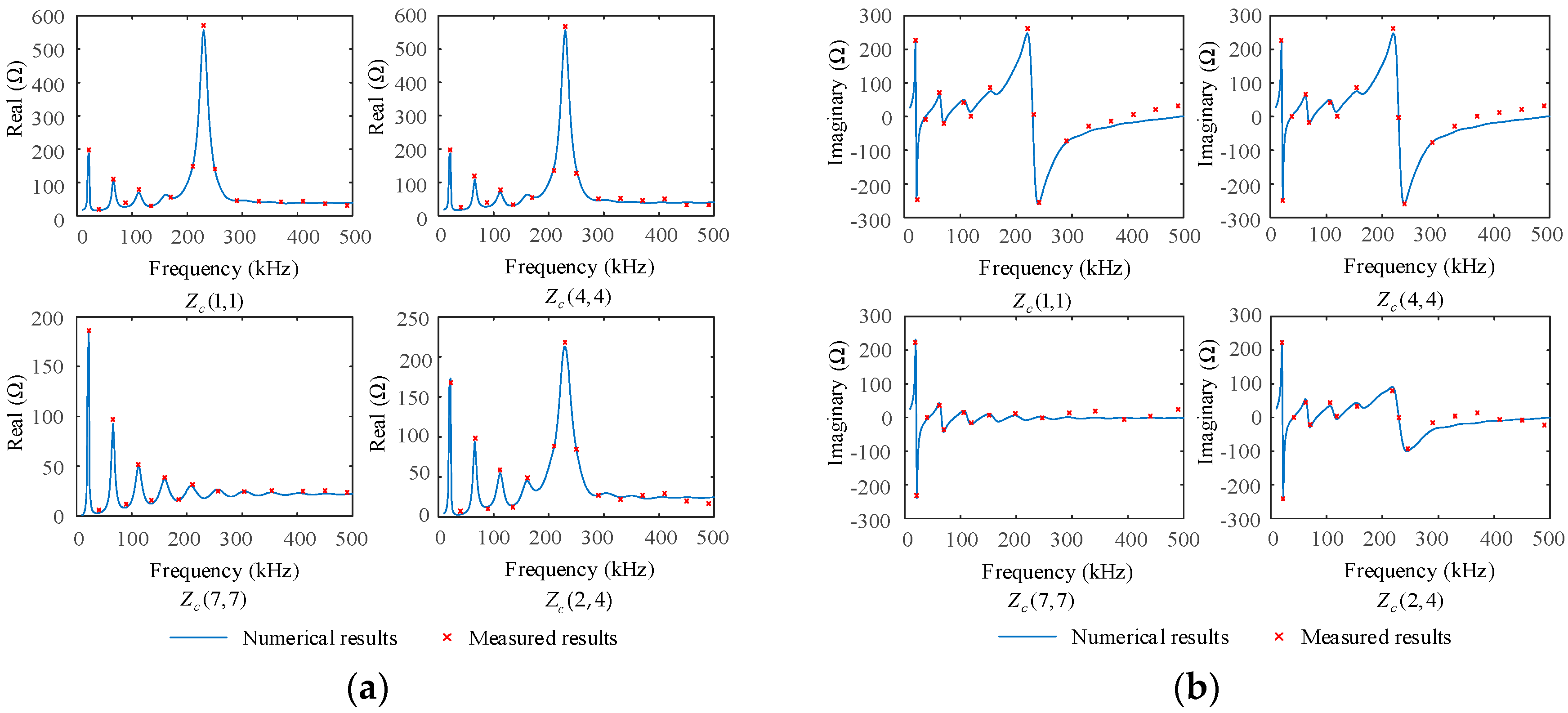
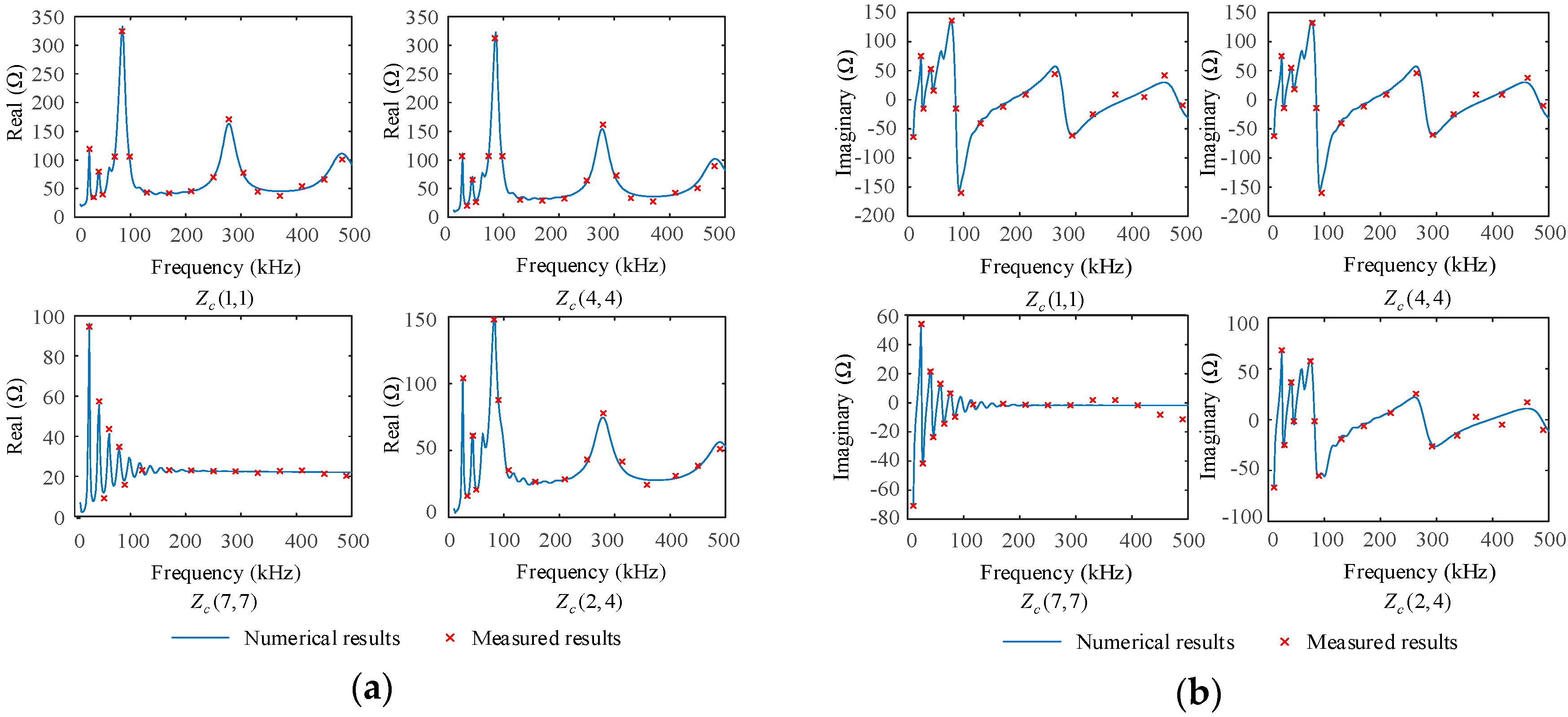
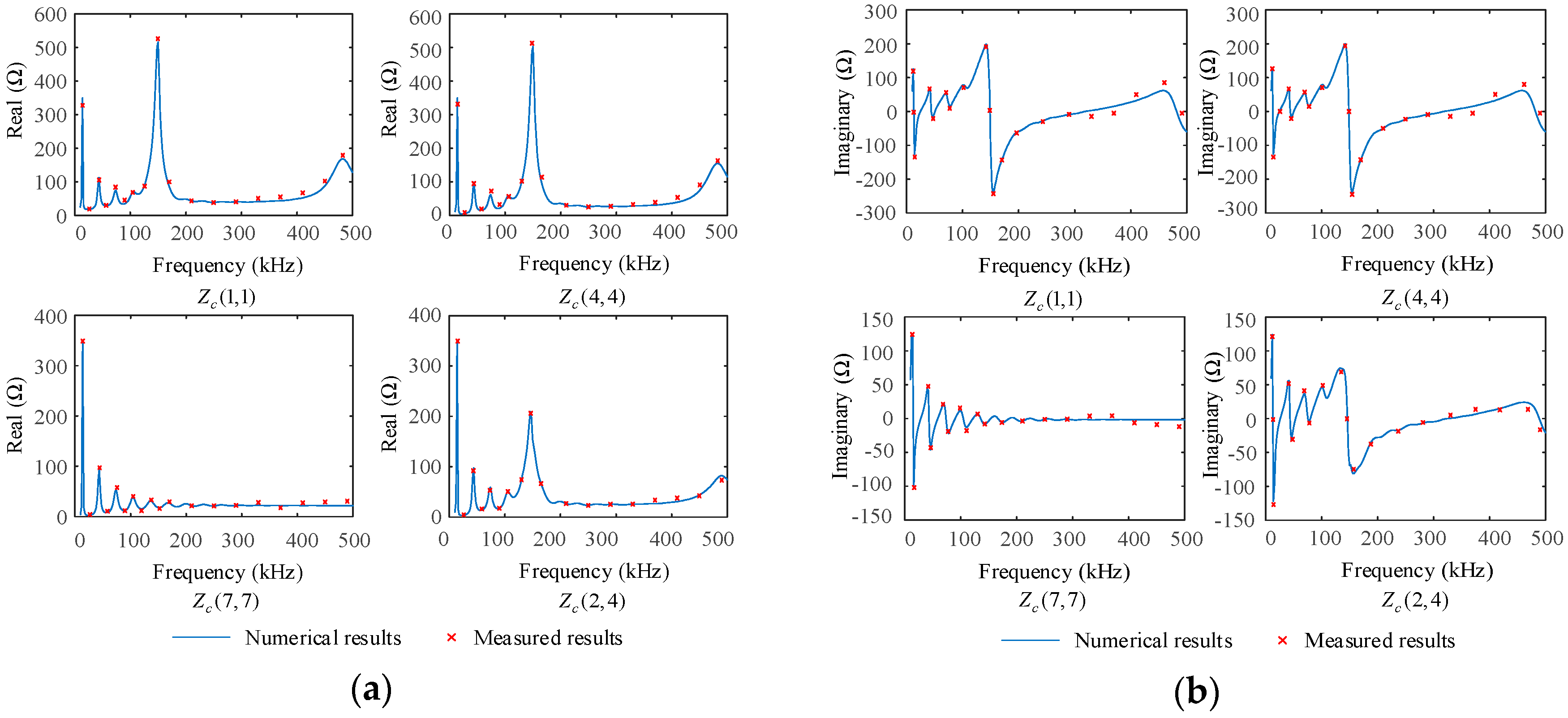
4. Method Validation
5. Analysis of the Characteristic Impedance Matrices
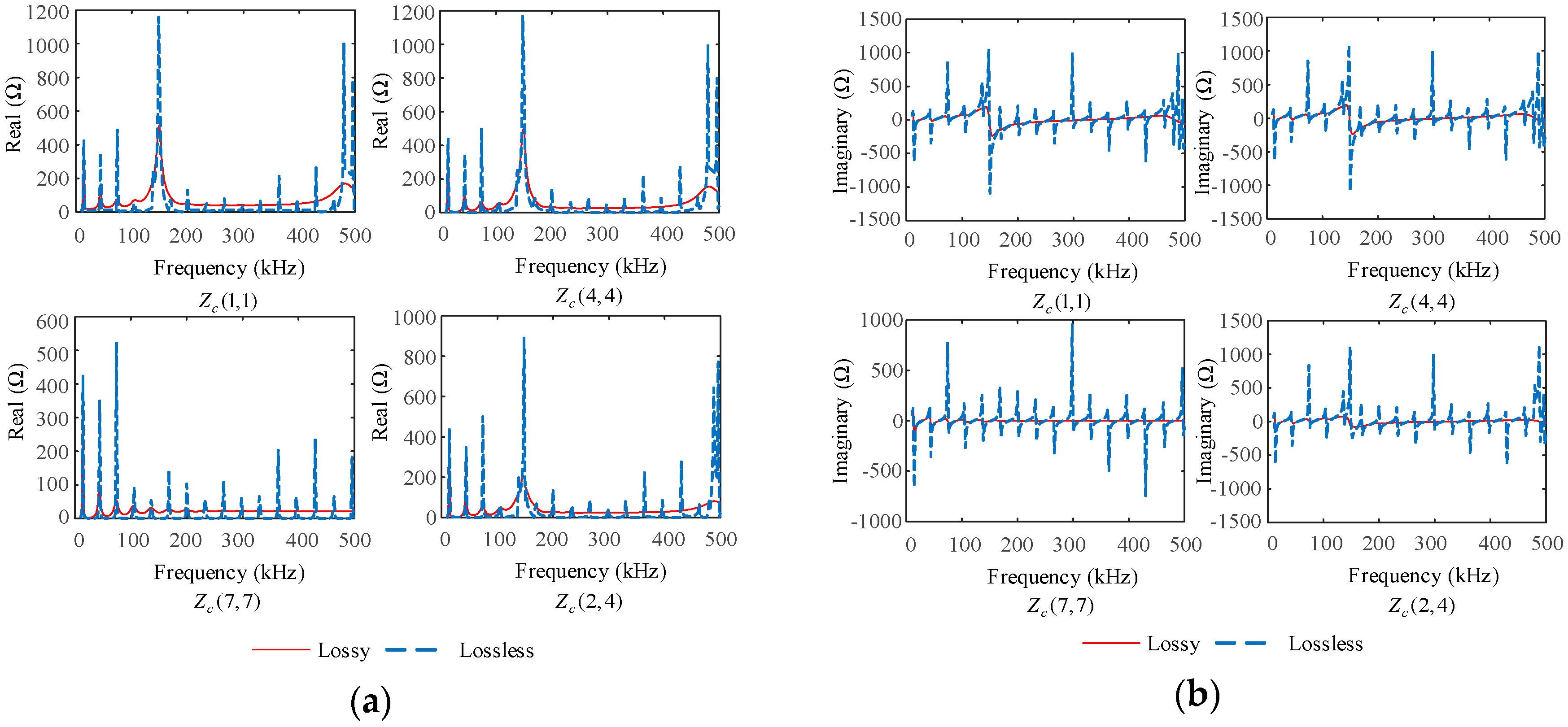
5.1. Characteristics of the Forward and Backward Characteristic Impedance Matrices
5.2. Effects of the Network Structures and Parameters
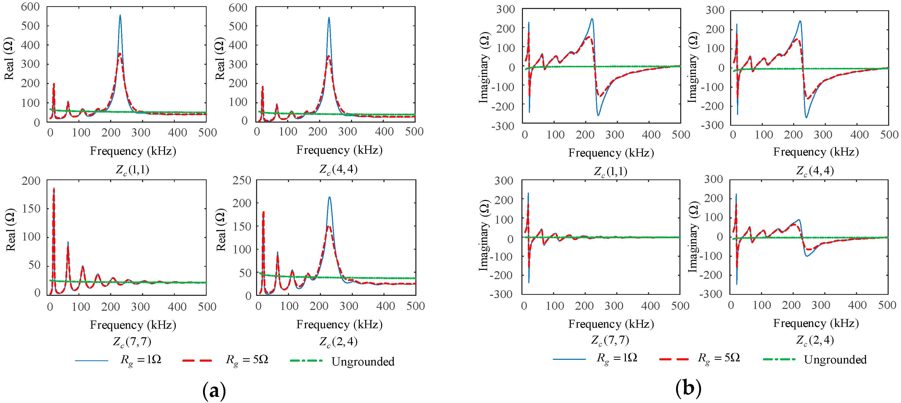
5.2.1. Effects of Grounding Resistances
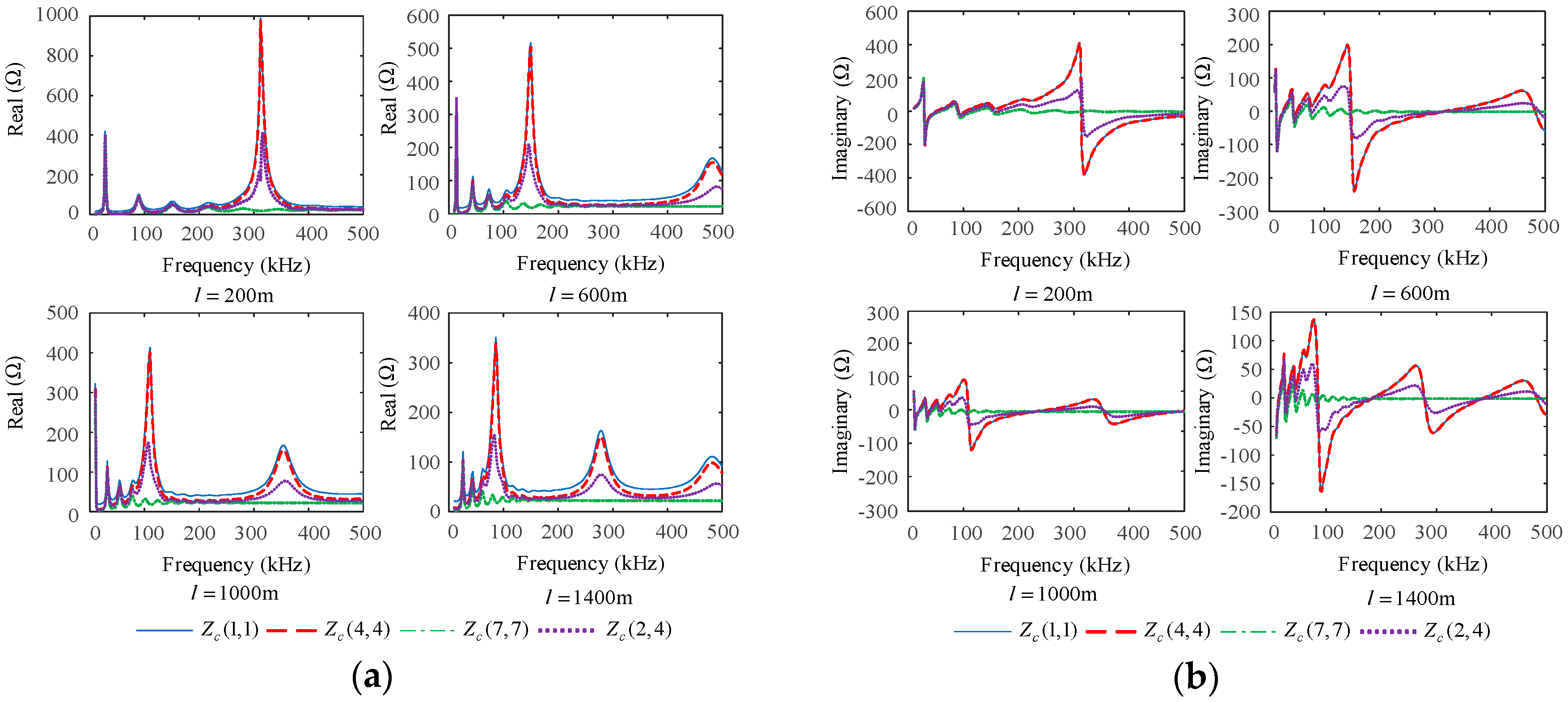
5.2.2. Effects of Cable Lengths
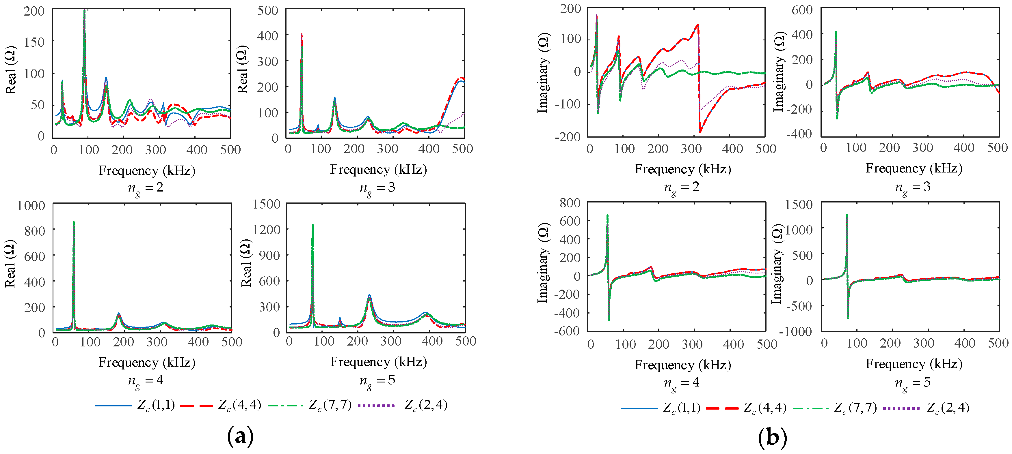
5.2.3. Effects of the Grounding Point Numbers
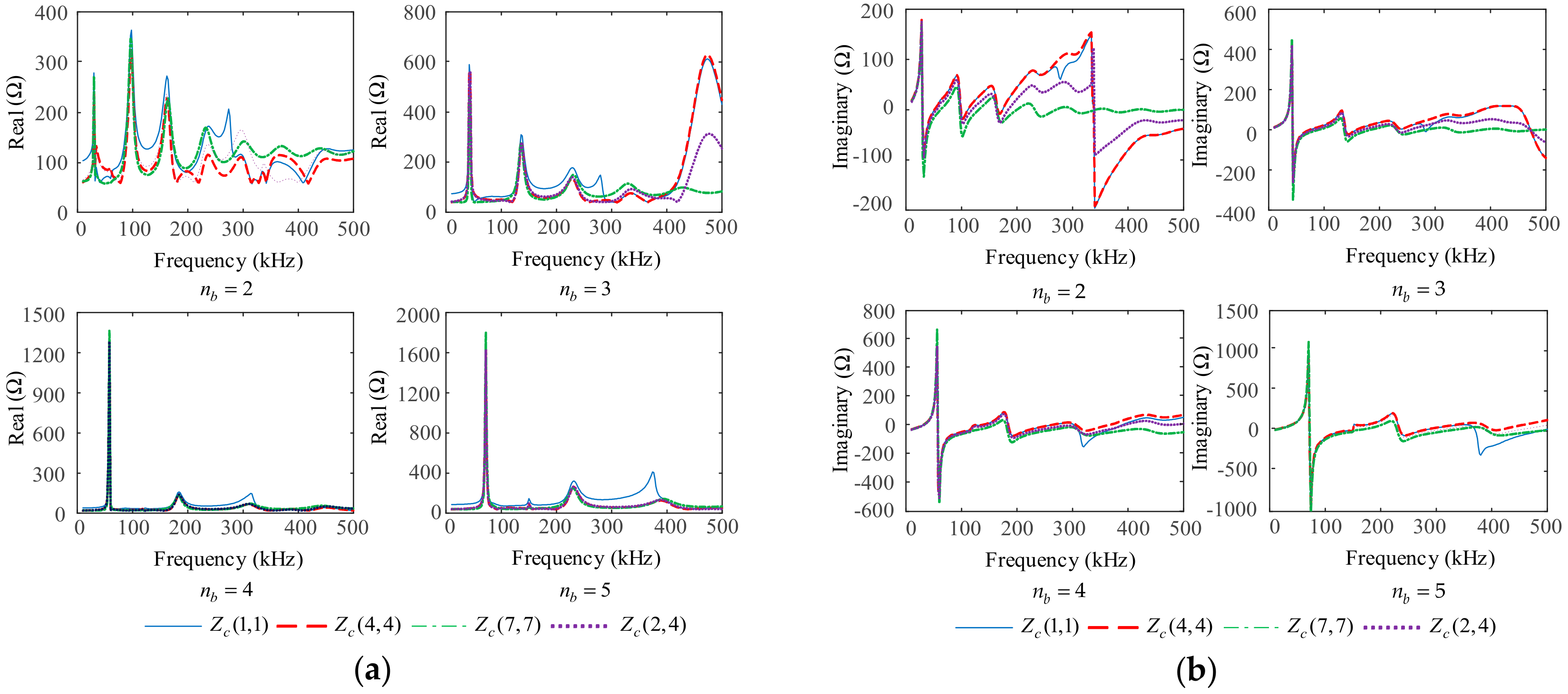
5.2.4. Effects of Cable Branch Numbers
6. Conclusions
- Considering the grounding of the shields and armors, the MV underground cables have FCIM and BCIM that were not equal unless the cables were longitudinally symmetrical. This is different from the case of uniform MV underground cables without grounding points, where the latter only has one unique characteristic impedance matrix.
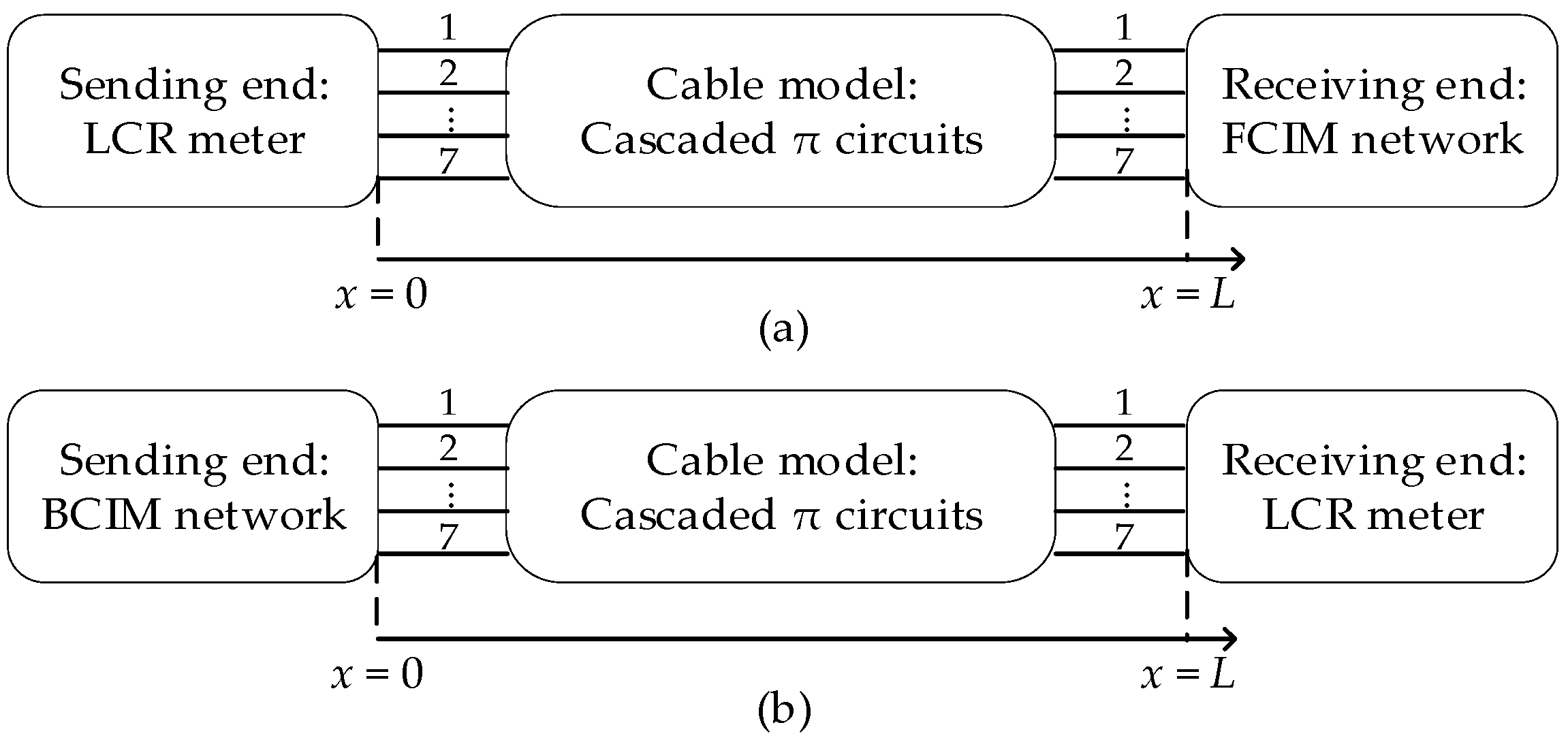
- If and only if the receiving end of the MV underground cable is connected to the FCIM, the access impedance matrix at the sending end is equal to the FCIM. Similarly, if and only if the sending end of the MV underground cable is connected to the BCIM, the access impedance matrix at the receiving end is equal to the BCIM.
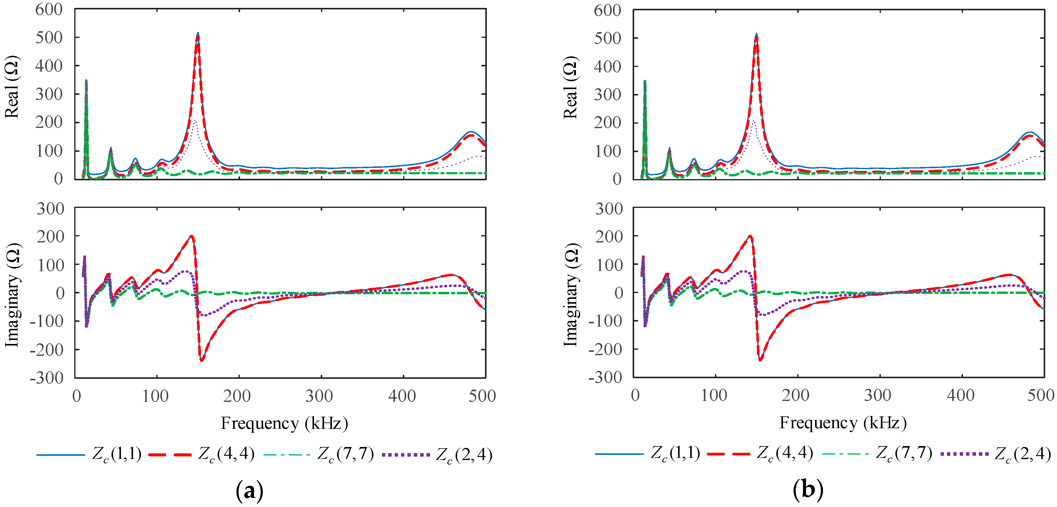
- The grounding of partial conductors will lead to resonance, resulting in multiple peaks in the characteristic impedances of the underground cables, which are not only reflected in the shields and armor, but can also be found in the cores. The resonance should be considered in investigations of the impedance matching for PLC to reduce or eliminate the reflected signal power at the transceivers.
- The smaller the grounding resistance, the larger the amplitudes at the resonant points. The grounding resistance does not affect the resonant frequencies. The longer the cable, the more resonant points in the fixed frequency range, and the smaller the amplitudes at the resonant points. The more grounding points along the cable, the fewer resonant points in the fixed frequency range, and the larger the amplitudes at the resonance points. Compared to the grounding of the shields and armor, the effects of well-matched cable branches on the characteristic impedance matrices are limited.
Author Contributions
Funding
Acknowledgments
Conflicts of Interest
Appendix A

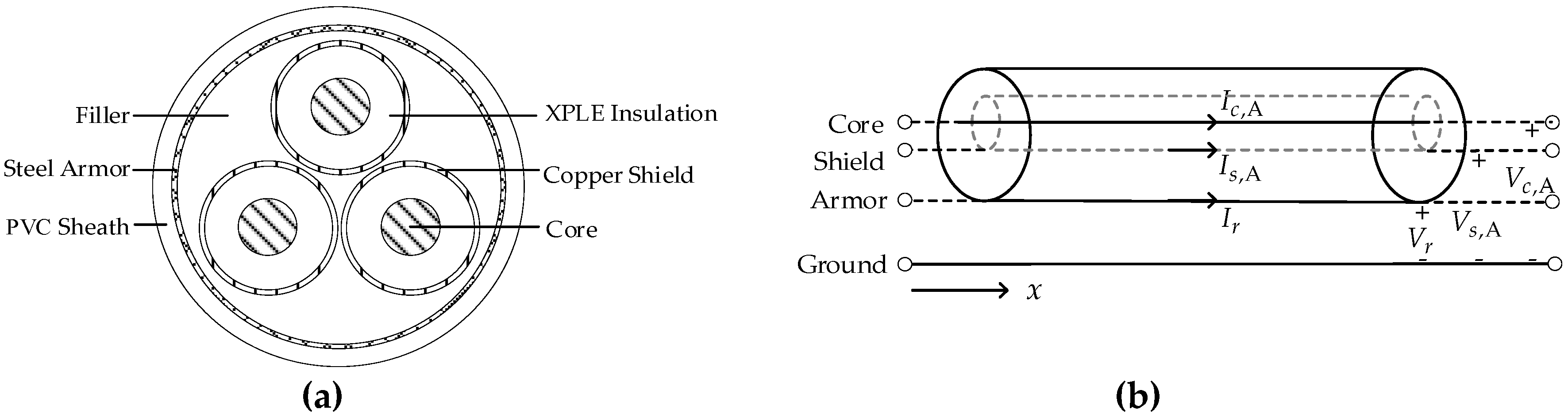
| Geometric Parameter | Radius (mm) | Electromagnetic Parameter | Value |
|---|---|---|---|
| Core conductor | 10.125 | Core or shield resistivity | 1.75 × 10⁻⁸ |
| Cross-linked polyethylene (XPLE) insulation | 15.325 | Armor resistivity | 9.78 × 10⁻⁸ |
| Copper shield | 15.925 | Insulation relative permittivity | 2.6 |
| Steel armor | 42.050 | Sheath relative permittivity | 6 |
| Polyvinyl chloride (PVC) sheath | 45.650 | Armor relative permeability 1 | 1000 |
Appendix B
References
- Shaukat, N.; Ali, S.M.; Mehmood, C.A.; Khan, B.; Jawad, M.; Farid, U.; Ullah, Z.; Anwar, S.M.; Majid, M. A survey on consumers empowerment, communication technologies, and renewable generation penetration within Smart Grid. Renew. Sustain. Energy Rev. 2018, 81, 1453–1475. [Google Scholar] [CrossRef]
- Chao, C.W.; Ho, Q.D.; Le-Ngoc, T. Challenges of power line communications for advanced distribution automation in smart grid. In Proceedings of the IEEE Power & Energy Society General Meeting, Vancouver, BC, Canada, 21–25 July 2013; pp. 1–5. [Google Scholar]
- Yang, L.; Crossley, P.A.; Wen, A.; Chatfield, R.; Wright, J. Design and performance testing of a multivendor IEC61850–9-2 process bus based protection scheme. IEEE Trans. Smart Grid 2014, 5, 1159–1164. [Google Scholar] [CrossRef]
- Hadbah, A.; Ustun, T.S.; Kalam, A. Using IEDScout software for managing multivendor IEC61850 IEDs in substation automation systems. In Proceedings of the IEEE International Conference on Smart Grid Communications, Venice, Italy, 3–6 November 2014; pp. 67–72. [Google Scholar]
- Emmanuel, M.; Rayudu, R. Communication technologies for smart grid applications: A survey. J. Netw. Comput. Appl. 2016, 74, 133–148. [Google Scholar] [CrossRef]
- Galli, S.; Scaglione, A.; Wang, Z. For the grid and through the grid: The role of power line communications in the smart grid. Proc. IEEE 2011, 99, 998–1027. [Google Scholar] [CrossRef]
- Sauter, T.; Lobashov, M. End-to-end communication architecture for smart grids. IEEE Trans. Ind. Electron. 2011, 58, 1218–1228. [Google Scholar] [CrossRef]
- Matanza, J.; Alexandres, S.; Rodríguez-Morcillo, C. Advanced metering infrastructure performance using European low-voltage power line communication networks. IET Commun. 2014, 8, 1041–1047. [Google Scholar] [CrossRef]
- Milioudis, A.N.; Andreou, G.T.; Labridis, D.P. Detection and location of high impedance faults in multiconductor overhead distribution lines using power line communication devices. IEEE Trans. Smart Grid 2015, 6, 894–902. [Google Scholar] [CrossRef]
- Della, G.D.; Ferrari, P.; Flammini, A.; Rinaldi, S.; Sisinni, E. Automation of distribution grids with IEC 61850: A first approach using broadband power line communication. IEEE Trans. Instrum. Meas. 2013, 62, 2372–2383. [Google Scholar]
- De, P.M.; Tonello, A.M. On impedance matching in a power-line-communication system. IEEE Trans. Circuits Syst. II Express Briefs 2016, 63, 653–657. [Google Scholar]
- Antoniali, M.; Tonello, A.M.; Versolatto, F. A study on the optimal receiver impedance for SNR maximization in broadband PLC. J. Electr. Comput. Eng. 2013, 2013, 1–11. [Google Scholar] [CrossRef]
- Paul, C.R. Analysis of Multi-Conductor Transmission Lines, 2nd ed.; John Wiley and Sons: Hoboken, NJ, USA, 2007. [Google Scholar]
- Costa, S.; de Queiroz, A.C.M.; Adebisi, B.; da Costa, V.L.R.; Ribeiro, M.V. Coupling for power line communications: A survey. J. Commun. Inform. Syst. 2017, 32, 8–22. [Google Scholar] [CrossRef]
- Van Rensburg, P.A.; Sibanda, M.P.; Ferreira, H.C. Integrated impedance-matching coupler for smart building and other power-line communications applications. IEEE Trans. Power Deliv. 2015, 30, 949–956. [Google Scholar] [CrossRef]
- Rui, C.P.; Barsoum, N.N.; Ming, A.W.; Ing, W.K. Adaptive impedance matching network with digital capacitor in narrowband power line communication. In Proceedings of the IEEE International Symposium on Industrial Electronics, Taipei, Taiwan, 28–31 May 2013; pp. 1–5. [Google Scholar]
- Hallak, G.; Bumiller, G. Data rate optimization on PLC devices with current controller for low access impedance. In Proceedings of the International Symposium on Power Line Communications and its Applications (ISPLC), Bottrop, Germany, 20–23 March 2016; pp. 144–149. [Google Scholar]
- Hallak, G.; Bumiller, G. Throughput optimization based on access impedance of PLC modems with limited power consumption. In Proceedings of the 2014 IEEE Global Communications Conference, Austin, TX, USA, 8–12 December 2014; pp. 2960–2965. [Google Scholar]
- Rasool, B.; Rasool, A.; Khan, I. Impedance characterization of power line communication networks. Arab. J. Sci. Eng. 2014, 39, 6255–6267. [Google Scholar] [CrossRef]
- Xiaoxian, Y.; Tao, Z.; Baohui, Z.; Fengchun, Y.; Jiandong, D.; Minghui, S. Research of impedance characteristics for medium-voltage power networks. IEEE Trans. Power Deliv. 2007, 22, 870–878. [Google Scholar] [CrossRef]
- Cataliotti, A.; Daidone, A.; Tinè, G. Power line communication in medium voltage systems: Characterization of MV cables. IEEE Trans. Power Deliv. 2008, 23, 1896–1902. [Google Scholar] [CrossRef]
- Yang, S.; Franklin, G. Effects of segmented shield wires on signal attenuation of power-line carrier channels on overhead transmission lines—Part I: Modeling method. IEEE Trans. Power Deliv. 2013, 28, 427–433. [Google Scholar] [CrossRef]
- Yang, S.; Franklin, G. Effects of segmented shield wires on signal attenuation of power-line carrier channels on overhead transmission lines—Part II: Signal attenuation results analysis. IEEE Trans. Power Deliv. 2013, 28, 434–441. [Google Scholar] [CrossRef]
- Araneo, R.; Celozzi, S.; Faria, J.A.B. Direct TD analysis of PLC channels in HV transmission lines with sectionalized shield wires. In Proceedings of the 2016 IEEE 16th International Conference on Environment and Electrical Engineering, Florence, Italy, 7–10 June 2016; pp. 1–4. [Google Scholar]
- Franklin, G.A. Using modal analysis to estimate received signal levels for a power-line carrier channel on a 500-kV transmission line. IEEE Trans. Power Deliv. 2009, 24, 2446–2454. [Google Scholar] [CrossRef]
- Wedepoh, L.M.; Mohamed, S.E.T. Multiconductor transmission lines: Theory of natural modes and fourier integral applied to transient analysis. Proc. Inst. Electr. Eng. 1969, 116, 1553–1563. [Google Scholar] [CrossRef]
- Wedepoh, L.M. Electrical characteristics of polyphase transmission systems, with special reference to boundary value calculations at power line carrier frequencies. Proc. Inst. Electr. Eng. 1965, 112, 2103–2112. [Google Scholar] [CrossRef]
- Perz, M.C. Natural modes of power line carrier on horizontal three phase lines. IEEE Trans. Power Appl. Syst. 1964, 83, 679–686. [Google Scholar] [CrossRef]
- Perz, M.C. A method of analysis of power line carrier problems on three-phase lines. IEEE Trans. Power Appl. Syst. 1964, 83, 686–691. [Google Scholar] [CrossRef]
- Wedepoh, L.M.; Wasley, R.G. Wave propagation in polyphase transmission systems: Resonance effects due to discretely bonded earth wires. Proc. Inst. Electr. Eng. 1965, 112, 2113–2119. [Google Scholar] [CrossRef]
- Faria, J.A.B.; da Silva, J.F.B. The effect of randomly earthed ground wires on PLC transmission: A simulation experiment. IEEE Trans. Power Deliv. 1990, 5, 1669–1677. [Google Scholar] [CrossRef]
- Olsen, R.G. Propagation along overhead transmission lines with multiply grounded shield wires. IEEE Trans. Power Deliv. 2017, 32, 789–798. [Google Scholar] [CrossRef]
- Rachidi, F.; Nucci, C.A.; Ianoz, M.; Mazzetti, C. Response of multiconductor power lines to nearby lightning return stroke electromagnetic fields. IEEE Trans. Power Deliv. 1997, 12, 1404–1411. [Google Scholar] [CrossRef]
- Correia de Barros, M.T.; Festas, J.; Almeida, M.E. Lightning induced overvoltages on multiconductor overhead lines. In Proceedings of the International Conference on Power Systems Transients, Budapest, Hungary, 20–24 June 1999; pp. 365–369. [Google Scholar]
- Andreotti, A.; Assante, D.; Verolino, L. Characteristic impedance of periodically grounded lossless multiconductor transmission lines and time-domain equivalent representation. IEEE Trans. Electromagn. Compat. 2014, 56, 221–230. [Google Scholar] [CrossRef]
- Araneo, R.; Faria, J.M.; Celozzi, S. Frequency-domain analysis of sectionalized shield wires on PLC transmission over high-voltage lines. IEEE Trans. Electromagn. Compat. 2017, 59, 853–861. [Google Scholar] [CrossRef]
- Faria, J.A.B.; Araneo, R. Computation, properties, and realizability of the characteristic immittance matrices of nonuniform multiconductor transmission lines. IEEE Trans. Power Deliv. 2018, 33, 1885–1894. [Google Scholar] [CrossRef]
- Faria, J.A.B.; Araneo, R. Matching a nonuniform MTL with only passive elements is not always possible. IEEE Trans. Power Deliv. 2019, 34, 467–474. [Google Scholar] [CrossRef]
- Benato, R.; Caldon, R. Distribution line carrier: Analysis and applications to DG. IEEE Trans. Power Deliv. 2007, 22, 575–583. [Google Scholar] [CrossRef]
- Lazaropoulos, A.G.; Cottis, P.G. Broadband transmission via underground medium-voltage power lines—Part I: Transmission characteristics. IEEE Trans. Power Deliv. 2010, 25, 2414–2424. [Google Scholar] [CrossRef]
- Ametani, A. A general formulation of impedance and admittance of cables. IEEE Trans. Power Appl. Syst. 1980, 99, 902–909. [Google Scholar] [CrossRef]
- Dommel, H.W. Electromagnetic Transients Program (EMTP Theory Book); Bonneville Power Administration: Portland, OR, USA, 1986; pp. 150–191.
- Schinzinger, R.; Ametani, A. Surge propagation characteristics of pipe enclosed underground cables. IEEE Trans. Power Appl. Syst. 1978, 5, 1680–1688. [Google Scholar] [CrossRef]
- Amekawa, N.; Nagaoka, N.; Ametani, A. Impedance derivation and wave propagation characteristics of pipe-enclosed and tunnel-installed cables. IEEE Trans. Power Deliv. 2004, 19, 380–386. [Google Scholar] [CrossRef]
- Wedepohl, L.M.; Wilcox, D.J. Transient analysis of underground power-transmission systems. System-model and wave-propagation characteristics. Proc. Inst. Electr. Eng. 1973, 120, 253–260. [Google Scholar] [CrossRef]


© 2019 by the authors. Licensee MDPI, Basel, Switzerland. This article is an open access article distributed under the terms and conditions of the Creative Commons Attribution (CC BY) license (http://creativecommons.org/licenses/by/4.0/).
Share and Cite
Zhao, H.; Zhang, W.; Wang, Y. Characteristic Impedance Analysis of Medium-Voltage Underground Cables with Grounded Shields and Armors for Power Line Communication. Electronics 2019, 8, 571. https://doi.org/10.3390/electronics8050571
Zhao H, Zhang W, Wang Y. Characteristic Impedance Analysis of Medium-Voltage Underground Cables with Grounded Shields and Armors for Power Line Communication. Electronics. 2019; 8(5):571. https://doi.org/10.3390/electronics8050571
Chicago/Turabian StyleZhao, Hongshan, Weitao Zhang, and Yan Wang. 2019. "Characteristic Impedance Analysis of Medium-Voltage Underground Cables with Grounded Shields and Armors for Power Line Communication" Electronics 8, no. 5: 571. https://doi.org/10.3390/electronics8050571
APA StyleZhao, H., Zhang, W., & Wang, Y. (2019). Characteristic Impedance Analysis of Medium-Voltage Underground Cables with Grounded Shields and Armors for Power Line Communication. Electronics, 8(5), 571. https://doi.org/10.3390/electronics8050571