Bistatic-ISAR Linear Geometry Distortion Alleviation of Space Targets

Abstract

The linear geometry distortion caused by time variant bistatic angles induces the sheared shape of the bistatic inverse synthetic aperture radar (bistatic-ISAR) image. A linear geometry distortion alleviation algorithm for space targets in bistatic-ISAR systems is presented by exploiting prior information. First, we analyze formation mathematics of linear geometry distortions in the Range Doppler (RD) domain. Second, we estimate coefficients of first-order polynomial of bistatic angles by least square error (LSE) method through exploiting the imaging geometry and orbital information of space targets. Third, we compensate the linear spatial-variant terms to restore the linear geometry distortions. Consequently, the restored bistatic-ISAR image with real shape is obtained. Simulated results of the ideal point scatterers dataset and electromagnetic numerical dataset verify the performance of the proposed algorithm.

1. Introduction

The monostatic inverse synthetic aperture radar (ISAR) system provides electromagnetic images of targets in the Range Doppler (RD) domain [1,2,3,4], which is suitable for the target recognition [5]. However, in monostatic ISAR systems, the image cannot be obtained when targets only move along the line of sight (LOS) of radar within the coherent process interval (CPI). To overcome this limitation, the bistatic configuration is introduced for the ISAR system [6]. In bistatic radar systems, the transmitting station and receiving station are separated spatially, and the length of the baseline is comparable to the distance of targets. The bistatic configuration is capable of obtaining complementary information of the target and providing better anti-jamming ability [6]. Hence, the bistatic-ISAR system has been an effective solution for space targets surveillance [7,8,9,10,11,12]. The bistatic-ISAR research, with respect to application and algorithm, has been studied in recent years [6,13,14,15,16,17,18,19].

Synchronization issues between the transmitting station and receiving station are inherent for the practical bistatic-ISAR configuration. Both the back-projection (BP) algorithm [20] and the polar-format-algorithm (PFA) [21] are sensitive to synchronization accuracy. Thus, applicability of those two algorithms is limited in bistatic-ISAR systems [13]. The RD imaging algorithm, with low requirement for synchronization accuracy and concise physical meaning, is widely used for simulated and real data process in bistatic-ISAR systems [6,8,14]. The bistatic equivalent monostatic (BEM) radar, an approximation of bistatic-ISAR systems, is derived, subject to certain constraints [14]. It effectively simplifies the bistatic-ISAR signal processing. The bistatic angle is the angle between the LOS of the transmitting station and receiving station. The time variant bistatic angles are caused by the bistatic configuration. However, the linear geometry/quadratic-defocusing distortions are caused by time variant bistatic angles when using the RD imaging algorithm [6,13,22].

In [16], a distortions mitigation algorithm based on “linked scatterers” to alleviate the distortions are introduced. However, this algorithm requires the transmitting station to work in duplex mode. Recently, a distortions mitigation algorithm was proposed in [22] by combining CPI reduction with super-resolution algorithms. However, the reduction factor of CPI needs to be deliberately calculated to guarantee that the distortions are less than corresponding resolution. Moreover, the tradeoff between distortion alleviation and resolution is required, even if using super resolution algorithms. In other words, higher resolution can be achieved in the same case, if the alleviation can be completed without reduction of CPI. Furthermore, the problem induced by the linear geometry distortion is more serious than the quadratic-defocusing one [23] in generic bistatic-ISAR systems. The linear geometry distortion causes a sheared target shape, since the linear Doppler shift of scatters in different range-bins change with the range position. It is almost impossible to perform target recognition with the sheared shape image. To alleviate the linear geometry distortions, the interferometric technique is adopted in bistatic-ISAR systems [24]. However, a super-receiver with at least three antennas needs to be configured for the interferometric technique. Both structure and complexity of the system are increased fast with an increasing antenna number, as compared with the classical bistatic-ISAR system with one transmitting station and one receiving station. Conversely, linear geometry distortion alleviation algorithms by exploiting prior information are promising solutions. In [25] we estimate the image distortion angle for space targets by exploiting prior information. By calculating the image distortion angle that we defined in [26], the linear geometry distortion alleviation is conducted in each range-bin. However, the assumption in [25] is that the space target position and the corresponding bistatic angle are completely accurate. In practical systems, there are errors of the satellite position data obtained by the telemetry network. Those errors are accumulated with slow time when calculating the image distortion angle. Hence, little error of the target position affects the subsequent image distortion alleviation. Further consideration of the linear geometry alleviation method should be discussed for practical bistatic-ISAR systems.

In this paper, we focus on the alleviation of linear geometry distortions and propose a corresponding alleviation algorithm of space targets through exploiting prior information in the classical bistatic-ISAR system. First, we calculate the bistatic angles through exploiting prior information (the imaging geometry and orbital information of space targets). Second, we obtain the coefficients of first-order polynomial of bistatic angles using the least square error (LSE) method. Then, we construct compensation in terms of the linear spatial-variant terms and conduct restoration the process based on phase compensation along each range-bin. Finally, we obtain the well-restored image with real shape via the compression and rescaling of cross range.

This paper is organized as follows. The bistatic-ISAR theories are revisited and related distortions are analytically treated in Section 2. The linear geometry distortion alleviation algorithm is discussed in detail in Section 3. In Section 4, simulated results using both the ideal point scatterers dataset and the electromagnetic numerical dataset are presented, respectively. In Section 5, we draw the conclusions.

2. Signal Model with Distortions

The generic bistatic radar configuration is shown in Figure 1. The transmitting station and receiving station are separated. $R_T$ and $R_R$ denote the distances between the target and the transmitting station and receiving station, respectively. The length of baseline $L$ is comparable with $R_T$ and $R_R$. The bistatic angle formed by bistatic radar geometry is referred as $\beta$.

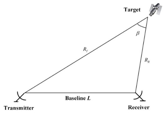
Figure 1. Generic bistatic radar configuration.

In the generic bistatic-ISAR system of the space target, assumptions of both the short CPI and far field are satisfied. The bistatic angle ${\beta }_m$ at $t_m$ and the distortion term $\cos {\beta }_m/2$ caused by the bistatic configuration can be represented as Equations (1) and (2) by first-order polynomial, respectively [6]:

$${\beta }_m\approx {\beta }_0+\Delta \beta t_m$$

(1)

where $t_m$ is slow time, ${\beta }_0=\beta (t_0)$ and $\Delta \beta ={\frac{d\beta (t_m)}{d{t}_m}|}_{t_m=0}$.

$$\cos \left(\frac{{\beta }_m}{2}\right)\approx \cos \left(\frac{{\beta }_0}{2}\right)-\frac{\Delta \beta }{2}\sin \left(\frac{{\beta }_0}{2}\right)t_m=K_0+K_1{t}_m$$

(2)

where

$$\begin{array}{cc}{K}_0=\cos \left(\frac{{\beta }_0}{2}\right)& K_1=-\frac{\Delta \beta }{2}\sin \left(\frac{{\beta }_0}{2}\right)\end{array}$$

(3)

The transmitted linear chirp modulation signal is as follows:

$$s_t\left(\widehat{t},t_m\right)=\mathrm{rect}\left(\frac{\widehat{t}}{T_p}\right)\exp \left[j2\pi \left(f_{c}t+\frac{1}{2}\mu {\widehat{t}}^2\right)\right]$$

(4)

where pulse repetition period is $T_{\mathrm{PRT}}$, the rectangle function is $\mathrm{rect}\left(u\right)=\{\begin{array}{c}1\left|u\right|\le \frac{1}{2}\\ 0\left|u\right|>\frac{1}{2}\end{array}$. $\widehat{t}=t-t_m$ denotes fast time. $T_p$ denotes pulse width. $f_c$ denotes carrier frequency. $\mu$ denotes chirp rate.

If constraint of the range-bin migration is satisfied, after successful signal pre-processing and translational motion compensation, the phase change between each period caused by both translational motion and the propagation of electromagnetic wave e.g., refractive effect, is compensated. The signal of the nth range-bin is written as Equation (5). More details are available in [6].

$$s_n(t_m)={\displaystyle \sum _{i=1}^{L_n}{A}_i\exp \left(\frac{-j4\mathsf{\pi }{f}_c}{c}\left(x_i{\omega }_0{t}_m+y_i\left(1-\frac{{\omega }_0^2{t}_m^2}{2}\right)\right)\left(K_0+K_1{t}_m\right)\right)}$$

(5)

where $(x_i,y_i)$ are the coordinates of the ith scatterer, $L_n$ is the scatterers number of the nth range-bin, $A_i$ is the complex amplitude and ${\omega }_0$ is the rotation velocity (RV).

The positions of range in Equation (5) are the same ($y_1=y_2=\cdots =y_{L_n}=y_n$). Neglecting the constant and third-order terms, $s_n(t_m)$ can be rewritten as follows:

$$s_n(t_m)={\displaystyle \sum _{i=1}^{L_n}{A}_i\exp \left(\frac{-j2\mathsf{\pi }{f}_c}{c}\left(2y_n{K}_1{t}_m+2{\omega }_0{x}_i{K}_0{t}_m+{\gamma }_i{t}_m^2\right)\right)}$$

(6)

where ${\gamma }_i=2{\omega }_0{x}_i{K}_1-y_n{K}_0{\omega }_0^2$.

Apply Fourier transform (FT) to $s_n(t_m)$ in Equation (6) along the slow-time direction.

$$\begin{array}{ll}{S}_n\left(f_d\right)& ={\displaystyle \underset{0}{\overset{T}{\int }}{s}_n(t_m)\exp (-j2\pi f_d{t}_m)d}{t}_m\\ & ={\displaystyle \sum _{i=1}^{L_n}{A}_{i}ps{f}_i\left(f_d-\left(f_i+\frac{2f_c{K}_1{y}_n}{c}\right)\right)}\end{array}$$

(7)

$T$ denotes the CPI. $f_d$ denotes the Doppler frequency. $f_i=2f_c{\omega }_0{x}_i{K}_0/c$ is the Doppler frequency of ith scatterer. $ps{f}_i(f_d)=T\sin \mathrm{c}(f_d)\otimes D_i(f_d)$ is the point spread function of ith scatterer. Symbol $\otimes$ denotes the convolution operator. $D_i(f_d)$ is the FT of the quadratic distortion terms of the ith scatterer.

$$D_i(f_d)={\displaystyle \underset{0}{\overset{T}{\int }}{A}_i\exp \left(\frac{-j2\mathsf{\pi }{f}_c}{c}{\gamma }_i{t}_m^2\right)\exp (-j2\pi f_d{t}_m)d}{t}_m$$

(8)

Because the quadratic distortion terms are relatively small in generic bistatic-ISAR systems [23], we focus on the linear distortion term. As expressed in Equation (7), scatterers cross-range positions are shifted by $2f_c{K}_1{y}_n/c$ along the cross-range direction in the nth range-bin. The shift of Doppler depends on the range position $y_n$ and leads to the sheared shape of bistatic-ISAR image.

3. Linear Geometry Distortion Alleviation Algorithm

3.1. Exploiting Prior Information

The configuration of bistatic-ISAR systems is shown in Figure 2. $\mathrm{Tx}$ and $\mathrm{Rx}$ represent the transmitting station and receiving station, respectively. The baseline length is referred to $L$. BEM radar is the instantaneous approximation of bistatic-ISAR system under certain constraints [6,14]. The target velocity is referred as $V$. $O$ is the target’s mass center. The distances between $O$ and the transmitting station and receiving station are $R_{TO}$ and $R_{RO}$ respectively. ${\beta }_0$ denotes initial bistatic angle at $t_0$. ${\zeta }_0$ denotes the initial view angle of the transmitting station at $t_0$. We establish the coordinate system $xOy$ according to the right hand rule. $O$ is the origin of $xOy$. Bisector of ${\beta }_0$ is the $y$ axis. $\left(x_P,y_P\right)$ are the coordinates of the scatterer $P$ in $xOy$. $d$ denotes the length of $OP$. The target’s mass center $O$ moves to $O_m$ at $t_m$. And the new coordinate system $x^{\prime }{O}_m{y}^{\prime }$ is translational motion of the old coordinate system $xOy$. ${\beta }_m$ denotes the bistatic angle of slow time $t_m$. ${\zeta }_m$ denotes the view angle of the transmitting station of slow time $t_m$. With the bisector of ${\beta }_m$ as $v$ axis and $O_m$ as the origin, we establish the coordinate system $u{O}_{m}v$ according to the right hand rule. $\left(x_{Pm},y_{Pm}\right)$ are the coordinates of the scatterer $P$ in the $u{O}_{m}v$. ${\alpha }_m$ is the angle between $O_m{P}_m$ and $u$ axis. ${\theta }_m$ is the change of equivalent view angle of BEM radar. The distances between $P_m$ and the transmitting station and receiving station are $R_{TPm}$ and $R_{RPm}$ respectively. The distances between $O_m$ and the transmitting station and receiving station are $R_{TOm}$ and $R_{ROm}$ respectively.

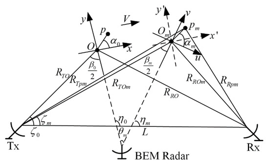
Figure 2. Imaging geometry of bistatic inverse synthetic aperture radar (bistatic-ISAR) system.

Two positions of the transmitting station and receiving station are known previously in the bistatic-ISAR system. Positions of the space targets can be calculated by combining the orbital motion model with precise ephemeris, as we mentioned in [10]. The precise ephemeris can be calculated from the telemetry data. Telemetry data can be achieved through fusing the radar and optical sensor results in telemetry network. $R_{TOm}$, $R_{ROm}$ and L can be calculated according to the geometry shown in Figure 2. Thus, the time variant bistatic angle ${\beta }_0$ and ${\beta }_m$, the corresponding view angles ${\zeta }_0$ and ${\zeta }_m$ can be obtained by the following equations:

$${\beta }_0=\arccos \left(\frac{R_{TO}^2+R_{RO}^2-L^2}{2R_{TO}{R}_{RO}}\right)$$

(9)

$${\beta }_m=\arccos \left(\frac{R_{TOm}^2+R_{ROm}^2-L^2}{2R_{TOm}{R}_{ROm}}\right)$$

(10)

$${\zeta }_0=\arccos \left(\frac{R_{TO}^2+L^2-R_{RO}^2}{2R_{TO}L}\right)$$

(11)

$${\zeta }_m=\arccos \left(\frac{R_{TOm}^2+L^2-R_{ROm}^2}{2R_{TOm}L}\right)$$

(12)

The corresponding ${\eta }_0$ and ${\eta }_m$ can be obtained by

$${\eta }_0={\zeta }_0+{\beta }_0/2$$

(13)

$${\eta }_m={\zeta }_m+{\beta }_m/2$$

(14)

The change of equivalent view angle of BEM radar ${\theta }_m$ (the equivalent rotation angle$\left({\alpha }_m-{\alpha }_0\right)$) is calculated by

$${\theta }_m={\eta }_0-{\eta }_m$$

(15)

As mentioned, the bistatic angle can be approximated by Equation (1) [${\beta }_m\approx {\beta }_0+\Delta \beta t_m$]. Therefore, we can estimate the ${\beta }_0$ and $\Delta \beta$ as $\widehat{{\beta }_0}$ and $\widehat{\Delta \beta }$ using the LSE method based on ${\beta }_m$, respectively. Then, we estimate $K_0$ and $K_1$ through the following equations respectively:

$${\widehat{K}}_0=\cos \left(\frac{\widehat{{\beta }_0}}{2}\right)$$

(16)

$${\widehat{K}}_1=-\frac{\widehat{\Delta \beta }}{2}\sin \left(\frac{\widehat{{\beta }_0}}{2}\right)$$

(17)

We obtain the estimated RV ${\widehat{\omega }}_0$ by the CPI and ${\theta }_m$. We should note ${\widehat{K}}_0$, ${\widehat{K}}_1$ and ${\widehat{\omega }}_0$ can be obtained with high accuracy. ${\xi }_{R_{TPm}}$ and ${\xi }_{R_{RPm}}$ (the errors of the distance $R_{TPm}$ and $R_{RPm}$) are relatively small compared with $R_{TPm}$ and $R_{RPm}$ and $L$ in the generic bistatic-ISAR system observing space targets. ${\xi }_{{\beta }_m}$ (the relative error of ${\beta }_m$) and ${\xi }_{{\theta }_m}$ (the relative error of ${\theta }_m$) are calculated according to the geometry shown in Figure 2. In this scenario, those two ${\xi }_{{\beta }_m}$ and ${\xi }_{{\theta }_m}$ are relatively small, e.g., ${\xi }_{{\beta }_m}=8.13\times 10{ }^{-6}$ and ${\xi }_{{\theta }_m}=8.61\times 10{ }^{-6}$, when ${\xi }_{R_{TPm}}=2 \mathrm{m}$, ${\xi }_{R_{RPm}}=2 \mathrm{m}$, $R_{TPm}=305.29 \mathrm{km}$, $R_{RPm}=603.45 \mathrm{km}$, and $L=800 \mathrm{km}$. The LSE method can find the optimum fitting coefficients of given data set. For more details, see our previous discussion in [27].

3.2. Compensation of Linear Spatial-Variant Phase Terms

As mentioned, the first order term $\exp \left(\frac{-j4\mathsf{\pi }{f}_c}{c}{y}_n{K}_1{t}_m\right)$ of the phase term depends on $y_n$ of the scatterers. It is the linear spatial-variant phase term. The range position $y_n$ is written with respect of range-bin index:

$$y_n=(n-n_c){\rho }_y$$

(18)

where $n$ represents the range-bin index of $y_n$ and $n_c$ represents the unknown index of range-bin of equivalent RC. Length of a sampling point along the direction of range ${\rho }_y$ can be written as [6]:

$${\rho }_y=\frac{c}{2f_s\cos \left({\beta }_0/2\right)}=\frac{c}{2f_s{K}_0}$$

(19)

where the $f_s$ is the sampling rate.

By substituting Equation (18) into Equation (6), the signal of the nth range-bin $s_n(t_m)$ becomes

$$s_n(t_m)={\displaystyle \sum _{i=1}^{L_n}{A}_i\exp \left(\frac{-j2\mathsf{\pi }{f}_c}{c}\left(2n{\rho }_y{K}_1{t}_m-2n_c{\rho }_y{K}_1{t}_m+2{\omega }_0{x}_i{K}_0{t}_m+{\gamma }_i{t}_m^2\right)\right)}$$

(20)

According to Equation (20), the linear geometry distortion is related to the $f_{c}n{\rho }_y{K}_1{t}_m/c$. We can estimate the coefficients $K_0$ ,$K_1$ and the ${\omega }_0$ in advanced by exploiting prior information. Therefore, we can construct the spatial-variant compensation term ${\phi }_c$ in Equation (21) to alleviate the distortion.

$${\phi }_{\mathrm{c}}=\exp \left(\frac{j4\mathsf{\pi }{f}_c}{c}n{\rho }_y{K}_1{t}_m\right)$$

(21)

Multiplying Equation (20) by Equation (21), the restoration of $s_n(t_m)$ can be written as

$${\overline{s}}_n(t_m)={\displaystyle \sum _{i=1}^{L_n}{A}_i\exp \left(\frac{-j2\mathsf{\pi }{f}_c}{c}\left(-2n_c{\rho }_y{K}_1{t}_m+2{\omega }_0{x}_i{K}_0{t}_m+{\gamma }_i{t}_m^2\right)\right)}$$

(22)

The FT of the restored ${\overline{s}}_n(t_m)$ are obtained as follows

$${\overline{S}}_n\left(f_d\right)={\displaystyle \sum _{i=1}^{L_n}{A}_{i}ps{f}_i\left(f_d-f_i-f_{rc}\right)}$$

(23)

where $f_i$ represents the Doppler frequency of ith scatterer defined in Equation (7) and $f_{rc}=-2f_c{K}_1{n}_c{\rho }_y/c$. $f_{rc}$ only leads to corresponding amount of shift of the slow time compression data over all range-bins. In turn, the shape of the target does not change with the unknown index of the range-bin of equivalent RC $n_c$. It does not need to estimate $n_c$. Thus, the restored image with correct shape can be obtained by the spatial-variant compensation term ${\phi }_c$ in Equation (21).

3.3. Algorithm Summary

The overall algorithm of the linear geometry distortion alleviation is summarized.

Step 1: Perform pulse compression along range direction and translational motion compensation on the received bistatic-ISAR signal and obtain the one-dimensional range profile expressed in Equation (6).

Step 2: Calculate time variant bistatic angles ${\beta }_m$ and change of the equivalent view angle of BEM radar ${\theta }_m$ (equivalent rotation angle), according to the geometry shown in Figure 2 and the positions of transmitting station, receiving station and space target (prior information).

Step 3: Estimate $\widehat{{\beta }_0}$ and $\widehat{\Delta \beta }$ based on ${\beta }_m$ by the LSE method, respectively. Calculate RV ${\widehat{\omega }}_0$ according to ${\theta }_m/CPI$. Calculate ${\widehat{K}}_0$ and ${\widehat{K}}_1$ according to Equations (16) and (17), respectively.

Step 4: Construct phase terms for compensation according to Equation (21) and compensate the signal $s_n(t_m)$ of each range-bin with the corresponding compensation term.

Step 5: Apply FT to the restored data along slow-time direction and obtain the rescale the image with ${\widehat{K}}_0$ and ${\widehat{\omega }}_0$ to display the real shape of the target.

4. Results and Discussion

We conduct the simulations based on an ideal point scatterers dataset using a space target model and an electromagnetic scattering dataset using a typical satellite model.

4.1. Simulation Setting

The simulation scenario is selected as follows. The transmitting station and receiving station are located at Beijing and Shanghai respectively. The International Space Station orbit is chosen as the simulation orbit. The two-line elements (TLE) of the International Space Station are shown in Table 1.

Table 1. Two-line elements (TLE) of the International Space Station (12 September 2018).

1 25544U 98067A   18255.09915832  .00001088  00000-0  23933-4 0  9999

2 25544  51.6419 305.5808 0005084 148.3817 299.1230 15.53835622132031

The International Space Station orbit is determined by its TLE data (provided by the Space-Surveillance-Network of America). The epoch time in the initial orbital elements is on 12 September 2018 at 02:22:47. The visible time-window of the bistatic-ISAR system is from 14:28:15 to 14:37:09 on 12 September 2018. We chose the particular CPI with the bistatic angle linear change from the visible time window as the imaging segment.

The simulation scenario is illustrated in Figure 3.

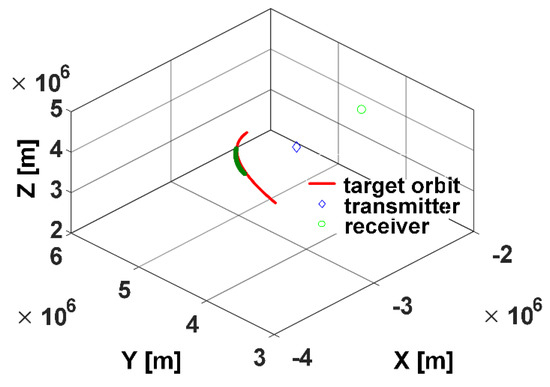
Figure 3. Simulation scenario.

The parameters of the bistatic-ISAR system are listed in Table 2.

Table 2. Parameters of the bistatic inverse synthetic aperture radar (bistatic-ISAR) system.

Parameter	Value	Parameter Name	Value
Carrier frequency	10 GHz	Sample frequency	800 MHz
Signal bandwidth	600 MHz	Pulse repetition frequency	100 Hz
Pulse width	20 us	Accumulated pulses	512
Integration angle	4.68°	Envelope alignment	Cross-correlation accumulation
Phase compensation	Phase gradient auto-focus	Image algorithm	Range Doppler
${\widehat{K}}_0$	0.7425	${\widehat{K}}_1$	−0.0073

4.2. Simulation Based on Two Datasets

The bistatic angles are calculated by the imaging geometry and the positions of the space target, transmitting station and receiving station. Figure 4 shows the change of bistatic angles with the pulse number within the CPI. Bistatic angles ${\beta }_m$ within the CPI almost change linearly with slow time. That is because the imaging segment is chosen with the bistatic angle linear change. Figure 5 shows the change of ${\theta }_m$ with the pulse number within the CPI. The rotation angle also changes linearly with slow time. The variation of the rotation angle is 4.68°. The equivalent RV is 0.016 rad/s.

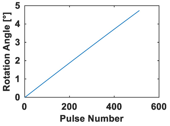
Figure 4. Bistatic angle ${\beta }_m$.

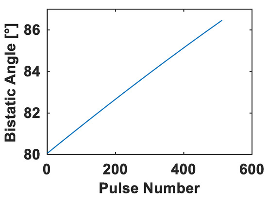
Figure 5. Equivalent rotation angle ${\theta }_m$.

The ideal point scatterer dataset of the space target shown in Figure 6a is comprised of 307 point scatterers. For the ideal point scatterer, scattering coefficient of each scatterer is 1. The typical satellite shown in Figure 7a has x, y and z extends of 40.09 m, 30.37 m, and 20.74 m, respectively. The ISAR image is the electromagnetic reflection of targets in the RD domain. It is dependent on the instantaneous radar cross section (RCS) distribution on the imaging plane. For further assessment of the proposed algorithm, the bistatic electromagnetic RCS dataset of the typical satellite is obtained by the numerical physical optics technique. The echo data corresponding to the two datasets respectively are generated by the method we proposed in [8].

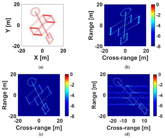
Figure 6. Results using the ideal point scatterers dataset: (a) The ideal point scatterers dataset (view of the line of sight (LOS) of bistatic equivalent monostatic (BEM) radar); (b) Before linear geometry distortion alleviation; (c) After linear geometry distortion alleviation with the proposed algorithm; (d) After linear geometry distortion alleviation with the algorithm in [25].

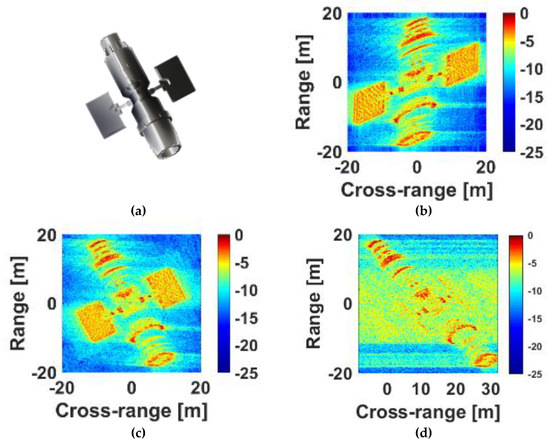
Figure 7. Results using the electromagnetic numerical radar cross section (RCS) dataset: (a) Computer aided design model of the satellite (the view of LOS of BEM radar); (b) Before linear geometry distortion alleviation; (c) After linear geometry distortion alleviation with the proposed algorithm; (d) After linear geometry distortion alleviation with the algorithm in [25].

The envelope alignment and the auto-focusing are achieved by the maximum cross-correlation algorithm and phase gradient auto-focus (PGA) algorithm, respectively. Then, the images of Figure 6b and Figure 7b are obtained by the RD imaging algorithm.

Due to the linear geometry distortion caused by time variant bistatic angles, the targets shape in Figure 6b and Figure 7b are sheared. Using the proposed linear geometry distortion alleviation algorithm, the linear geometry distortions are alleviated in Figure 6c and Figure 7c (compare Figure 6b with Figure 6c, compare Figure 7b with Figure 7c). The shape of the targets in the restored Figure 6c and Figure 7c are consistent with the corresponding ones in Figure 6a and Figure 7a (view of the LOS of BEM radar), respectively. It is beneficial to targets recognition.

The real shape of the target cannot be obtained by the algorithm in [25] and the image of several range-bins is defocused (Figure 6d and Figure 7d). The reason is that the assumption of complete accurate prior information is not satisfied in practical system and the image distortion angle is sensitive to the errors of prior information. Meanwhile, the results of the electromagnetic numerical dataset of typical satellite in Figure 7 and the comparison between proposed algorithm and the algorithm in [25] further verified the robustness of the presented algorithm.

5. Conclusions

We present a clear procedure of the linear geometry distortion alleviation algorithm based on prior information for better utilization of the bistatic-ISAR image. Simulated results of both ideal point scatterer dataset of space target model and electromagnetic numerical dataset of the typical satellite model verify the feasibility and robustness of proposed algorithm. The comparisons of the results before and after the alleviation indicate that our algorithm is capable of restoring the linear geometry distortion and providing the real shape of the target. The restored results are beneficial to further target classification and recognition.

References

- Walker, J.L. Range-doppler imaging of rotating objects. IEEE Trans. Aerosp. Electron. Syst. 1980, 16, 23–52. [Google Scholar] [CrossRef]
- Xing, M.; Wu, R.; Li, Y.; Bao, Z. New ISAR imaging algorithm based on modified Wigner-Ville distribution. IET Radar Sonar Navig. 2008, 3, 70–80. [Google Scholar] [CrossRef]
- Zhao, J.; Zhang, M.; Wang, X.; Cai, Z.; Nie, D. Three-dimensional super resolution ISAR imaging based on 2D unitary ESPRIT scattering centre extraction technique. IET Radar Sonar Navig. 2017, 11, 98–106. [Google Scholar] [CrossRef]
- Lv, Y.; Wu, Y.; Wang, H.; Qiu, L.; Jiang, J.; Sun, Y. An Inverse Synthetic Aperture Ladar Imaging Algorithm of Maneuvering Target Based on Integral Cubic Phase Function-Fractional Fourier Transform. Electronics 2018, 7, 148. [Google Scholar] [CrossRef]
- Giusti, E.; Martorella, M.; Capria, A. Polarimetrically-Persistent-Scatterer-Based Automatic Target Recognition. IEEE Trans. Geosci. Remote Sens. 2011, 49, 4588–4599. [Google Scholar] [CrossRef]
- Martorella, M.; Palmer, J.; Homer, J.; Littleton, B.; Longstaff, D. On bistatic inverse synthetic aperture radar. IEEE Trans. Aerosp. Electron. Syst. 2007, 43, 1125–1134. [Google Scholar] [CrossRef]
- Bai, X.; Zhou, F.; Xing, M.; Bao, Z. Scaling the 3-D Image of Spinning Space Debris via Bistatic Inverse Synthetic Aperture Radar. IEEE Geosci. Remote Sens. Lett. 2010, 7, 430–434. [Google Scholar] [CrossRef]
- Guo, B.F.; Shang, C.X.; Wang, J.L. Bistatic ISAR echo simulation of space target based on two-body model. Syst. Eng. Electron. 2016, 38, 1771–1779. [Google Scholar] [CrossRef]
- Ma, J.; Gao, M.; Hu, W.; Di, X.; Shi, L. Optimum Distribution of Multiple Location ISAR and Multi-angles Fusion Imaging for Space Target. J. Electron. Inf. Technol. 2017, 39, 2834–2843. [Google Scholar] [CrossRef]
- Ma, J.T.; Gao, M.G.; Guo, B.F.; Dong, J.; Xiong, D.; Feng, Q. High resolution inverse synthetic aperture radar imaging of three-axis-stabilized space target by exploiting orbital and sparse priors. Chin. Phys. B 2017, 26, 108401. [Google Scholar] [CrossRef]
- Tian, B.; Zou, J.; Xu, S.; Chen, Z. Squint model interferometric ISAR imaging based on respective reference range selection and squint iteration improvement. IET Radar Sonar Navig. 2015, 9, 1366–1375. [Google Scholar] [CrossRef]
- Han, N.; Li, B.; Wang, L.; Tong, J.; Guo, B. Algorithm for autofocusing of bistatic ISAR of space target based on sparse decomposition. Acta Aeronaut. Astronaut. Sin. 2018, 39, 322037. [Google Scholar] [CrossRef]
- Martorella, M. Analysis of the Robustness of Bistatic Inverse Synthetic Aperture Radar in the Presence of Phase Synchronisation Errors. IEEE Trans. Aerosp. Electron. Syst. 2011, 47, 2673–2689. [Google Scholar] [CrossRef]
- Martorella, M.; Cataldo, D.; Brisken, S. Bistatically equivalent monostatic approximation for bistatic ISAR. In Proceedings of the IEEE Radar Conference, Ottawa, ON, Canada, 29 April–3 May 2013; pp. 1–5. [Google Scholar]
- Shi, L.; Guo, B.F.; Ma, J.T.; Shang, C.X.; Zeng, H.Y. A Novel Channel Calibration Method for Bistatic ISAR Imaging System. Appl. Sci. 2018, 8, 2160. [Google Scholar] [CrossRef]
- Sun, S.B.; Jiang, Y.C.; Yuan, Y.S.; Hu, B.; Yeo, T.S. Defocusing and distortion elimination for shipborne bistatic ISAR. Remote Sens. Lett. 2016, 7, 523–532. [Google Scholar] [CrossRef]
- Xiong, D.; Zhang, X.; Wang, J.; Zhao, H.; Gao, M. Reception and calibration of bistatic SF ISAR imaging system with wideband receiver. IET Radar Sonar Navig. 2017, 11, 379–385. [Google Scholar] [CrossRef]
- Zhang, S.S.; Sun, S.B.; Zhang, W.; Zong, Z.L.; Yeo, T.S. High-Resolution Bistatic ISAR Image Formation for High-Speed and Complex-Motion Targets. IEEE J. Sel. Top. Appl. Earth Obs. Remote Sens. 2015, 8, 3520–3531. [Google Scholar] [CrossRef]
- Zhao, L.; Gao, M.; Martorella, M.; Stagliano, D. Bistatic three-dimensional interferometric ISAR image reconstruction. IEEE Trans. Aerosp. Electron. Syst. 2015, 51, 951–961. [Google Scholar] [CrossRef]
- Chen, S.; Zhao, H.C.; Zhang, S.N.; Chen, Y. An improved back projection imaging algorithm for dechirped missile-borne SAR. Acta Phys. Sin. 2014, 62, 218405. [Google Scholar] [CrossRef]
- Horvath, M.S.; Gorham, L.A.; Rigling, B.D. Scene Size Bounds for PFA Imaging with Postfiltering. IEEE Trans. Aerosp. Electron. Syst. 2013, 49, 1402–1406. [Google Scholar] [CrossRef]
- Cataldo, D.; Martorella, M. Bistatic ISAR Distortion Mitigation via Superresolution. IEEE Trans. Aerosp. Electron. Syst. 2018, 54, 2143–2157. [Google Scholar] [CrossRef]
- Jiang, Y.; Sun, S.; Yeo, T.S.; Yuan, Y. Bistatic ISAR distortion and defocusing analysis. IEEE Trans. Aerosp. Electron. Syst. 2016, 52, 1168–1182. [Google Scholar] [CrossRef]
- Ma, C.Z.; Yeo, T.S.; Guo, Q.; Wei, P.J. Bistatic ISAR Imaging Incorporating Interferometric 3-D Imaging Technique. IEEE Trans. Geosci. Remote Sens. 2012, 50, 3859–3867. [Google Scholar] [CrossRef]
- Guo, B.F.; Shang, C.X.; Wang, J.L.; Gao, M.G.; Fu, X.J. Correction of migration through resolution cell in bistatic inverse synthetic aperture radar in the presence of time variant bistatic angle. Acta Phys. Sin. 2014, 63, 238406. [Google Scholar]
- Dong, J.; Gao, M.G.; Shang, C.X.; Fu, X.J. The Image Plane Analysis and Echo Model Amendment of Bistatic ISAR. J. Electron. Inf. Technol. 2010, 32, 1855–1862. [Google Scholar] [CrossRef]
- Zhu, X.X.; Hu, W.H.; Ma, J.T.; Guo, B.F.; Xue, D.F. ISAR autofocusing imaging with sparse apertures and time variant bistatic angle. Acta Aeronaut. Astronaut. Sin. 2018, 39, 322059. [Google Scholar] [CrossRef]
© 2019 by the authors. Licensee MDPI, Basel, Switzerland. This article is an open access article distributed under the terms and conditions of the Creative Commons Attribution (CC BY) license (http://creativecommons.org/licenses/by/4.0/).