1. Introduction
Sound source and speech recognition technologies have been developed and used with various techniques utilizing microphone array. The magnitude of the sound signal arriving at the microphone is inversely proportional to the square of the distance from the microphone to the sound source. Normally, sound source detection for long distances is not feasible, because the sound signal is so susceptible to environmental noise. The sound signal experiences reflection, diffraction, and interferences with respect to the environment conditions, such as air temperature, existence of obstacles, size of the space, and surrounding sound signals, which cause signal distortions and degrade the reliability of the signal [
1,
2].
To obtain a specific value for a sound signal, the method of extracting maximum or threshold value has the advantage of requiring fewer calculations and being faster. However, it has the disadvantage of not being effective in environments with noise. On the other hand, to analyze the similarity between signals, a difference method, cross correlation, and generalized cross correlation are applied, which can demonstrate strong and robust performance even in noisy environments. The sound source location has been estimated by mapping the cross-correlation function onto a geometrical space instead of using the time difference function [
3,
4]. Additionally, head-related transfer function (HRTF), beam forming method (BFM), and artificial ear method (AEM) have been used to detect the sound source localization for robotics areas. However, most of these methods require heavy computations and are expensive for use in robotic applications [
5,
6].
Due to the fact that sound location recognition technology is very weak and not stable enough to be applied to actual robots, most studies have been conducted with an emphasis on signal processing that analyzes specific signals. Currently, based on these studies, technology and equipment have been developed to recognize sound sources that are fairly stable. Therefore, sound localization recognition technology has been applied and studied with respect to robotic systems. One of these areas is the application of mobile robots, and there is research on such robots moving and following markers to recognized locations, engaging in obstacle avoidance, etc. [
7,
8]. In particular, sound-position recognition mobile robots follow a sound source from any position using abnormal speed changes and rapid rotation of the mobile robot’s trajectory. Thus, the interaction between the target point, the moving robot, and the surrounding obstacles is very important in order for the robot to recognize and follow the moving sound source in real time and to avoid the obstacle.
Several studies have examined real-time obstacle avoidance using techniques, such as vector field histogram (VFH) approach, curvature velocity method (CVM), and dynamic window approach (DWA), which have local minima that can be avoided with certain modifications [
9,
10,
11]. The potential field method (PFM) has been proposed to generate an attraction force to the target and a repulsive force against an obstacle to determine the direction and velocity of the mobile robot [
12,
13,
14,
15,
16,
17,
18].
In this paper, the virtual impedance method has been adopted and elaborated to improve obstacle avoidance performance [
15]. The relationship between the uncertain environment and the mobile robot has been modeled as an impedance formed by the damper and spring, which generates a potential vector for the mobile robot [
16,
17,
18,
19,
20]. The conventional virtual impedance algorithm may be confronted with a local minimum during navigation by the obstacles with fixed coefficients of the impedance. In this study, the impedance coefficients have been adjusted dynamically to improve the collision avoidance performance, and the scheme is called the active virtual impedance method. The location of the sound source has been estimated based on the TDOA (Time Difference of Arrival), and the virtual impedance algorithm has been applied to allow a mobile robot to follow a sound and avoid obstacles.
This paper is organized in six sections.
Section 2 explains how to estimate the location of the sound source. In
Section 3, the main idea of this paper, the active virtual impedance algorithm, is proposed. The experimental systems of the mobile robot and sensors are illustrated in
Section 4, and the experimental results are discussed in
Section 5. Finally,
Section 6 presents our conclusions.
2. Localization of Sound Source
2.1. Point Sound Source
Generally, sound waves are caused by vibrations of objects. We can use speakers or horns as sound sources to artificially generate sounds that are meant to occur at a time interval with a given rule to warn or to indicate a location. A sound that generates instantaneous sound in a relatively short time is a form of short-term energy release.
This type of sound source has relatively clear boundaries between the parts with and without sound waves.
The frequency of sound,
f, traveling with the velocity
can be changed to
f’ by the relative velocity at the observer point using the Doppler formula as follows:
where
and
represent the velocity of the observer and sound source, respectively.
is the propagation velocity of the sound. The Doppler effect can be ignored when
and
, i.e., the velocities of the sound source and the mobile robot are considerably smaller than the propagation velocity of sound. Diffusion, diffraction, and reflection of the sound signal in the environment make the signal recognition for the localization difficult.
The sound signal velocity, , is 340 m/s in the air at room temperature. Using this velocity and traveling time, the distance between the sound source and microphone can be calculated.
2.2. Arriving Time Difference Method
The distance from the sound source to
microphone,
, can be obtained as follows:
where
is the traveling time of the sound source to the
microphone.
For the two received signals
and
, the
sampling data can be expressed as:
The similarity function,
, can be defined from these two data sets as follows:
When the signal
is shifted
steps, the similarity function can be represented as:
where
is
. Using Equation (5),
, which gives the maximum similarity value, can be obtained. The arrival time difference between the two signals
can be calculated using
and the sampling period, which is represented as:
where
represents the sampling period of the data sets.
2.3. Recognition of Sound Source
For the simplicity of obtaining the distances, , and angles, to the sound source, three microphones, , , and were installed on the same plane at a constant interval ().
2.3.1. Distance Estimation in Two-Dimensional (2D) Space
In
Figure 1, the geometrical relationships of
, and
to
can be represented, respectively, as follows:
where
represents the traveling time of the sound source to the
microphone, and
and
represent the arrival time difference between two microphones, 1–2 and 1–3, respectively.
In
Figure 1, the distance to the sound source, D, can be obtained using the triangular area formula. Using Heron’s formula, the areas of two triangles,
and
, can be obtained as follows:
where
.
The two areas are actually the same. By placing this relation into Equation (7), the distance
can be obtained as follows:
2.3.2. Angle Estimation in 2D Space
The distance to the sound source from the microphone is much larger than the interval between the microphones. Therefore, the traveling path of the sound signal can be approximated as parallel lines, as shown in
Figure 2. Using the cosine laws, the orientation angle,
, can be estimated when the arrival time differences,
, are available.
The arrival angle of the sound signal can be calculated as follows:
where
is the difference of
and
, which are distances from microphones 1 and 2 to the sound source, respectively. The angle can be also calculated as follows:
where
is the difference of
and
, which are distances from microphones 2 and 3 to the sound source, respectively.
2.4. Performance Evaluation of Sound Source Recognition
To check the performance of the sound source recognition using the microphone array, sound source detecting experiments were performed in a wide, obstacle-free, indoor environment. The distance between the sound source and microphone array, D, was selected as 1, 2, 3, and 4 m, whereas the angle,
, was selected to be 0, 30, and 60°.
Table 1 lists the mean values of D and
from 100 measurements.
Table 2 summarizes the standard deviations of the measurements for distances and angles.
An analysis of
Table 1 and
Table 2 reveal an increase in the errors in measuring the distance and angle with increasing distance. In addition, the error also increased with the increasing angle between the sound source and microphones,
. With increasing D and
, the possibility of signal distortion became larger and the intensity of the signal became weaker, which caused measurement difficulties and errors.
3. Obstacle Avoidance Using Active Virtual Impedance
For the navigation robot to avoid obstacles more efficiently, a new active virtual impedance algorithm is proposed here.
3.1. Collision Vector and Rotation
For a mobile robot to avoid obstacles during navigation, the locations of the obstacles need to be identified first. The distance vector from the sensor to an object,
(
: integer), can be defined as:
where
represents the distance to an obstacle from the
sensor;
represents the angle between the robot moving direction
and
sensor, and (
,
) represent the location of the
sensor. To detect obstacles in front of the mobile robot, three distance sensors were attached in front of the mobile robot. A collision vector,
is defined using the sense data. Two different situations occur when defining the collision vector.
[Case I] When the obstacle is small, it can be detected only by a distance sensor. In this case, the collision vector,
is defined as:
[Case II] When the obstacle is detected by two distance sensors, the collision vector,
can be defined using two pointing vectors,
and
. From the two pointing vectors, as shown in
Figure 3, two obstacle vectors
and
can be obtained as follows:
The line between the two points,
and
can be obtained and represented as
. Then, a collision vector from the mobile robot to an obstacle can be defined as
, which is vertical to the line
from the origin of the mobile robot,
. Thus, the collision vector,
, is defined as follows:
where
and
is defined as the origin of the sensors with respect to a world frame.
The collision vector is defined with respect to the mobile robot frame, which needs to be transformed to a world frame to drive to the mobile robot into a target position specified with respect to the world frame.
As shown in
Figure 4, the orientation of the mobile robot can be transformed into the world frame by rotating
along the
-axis as follows.
Therefore, the collision vector can be represented with respect to the world frame as follows:
3.2. Virtual Impedance Model
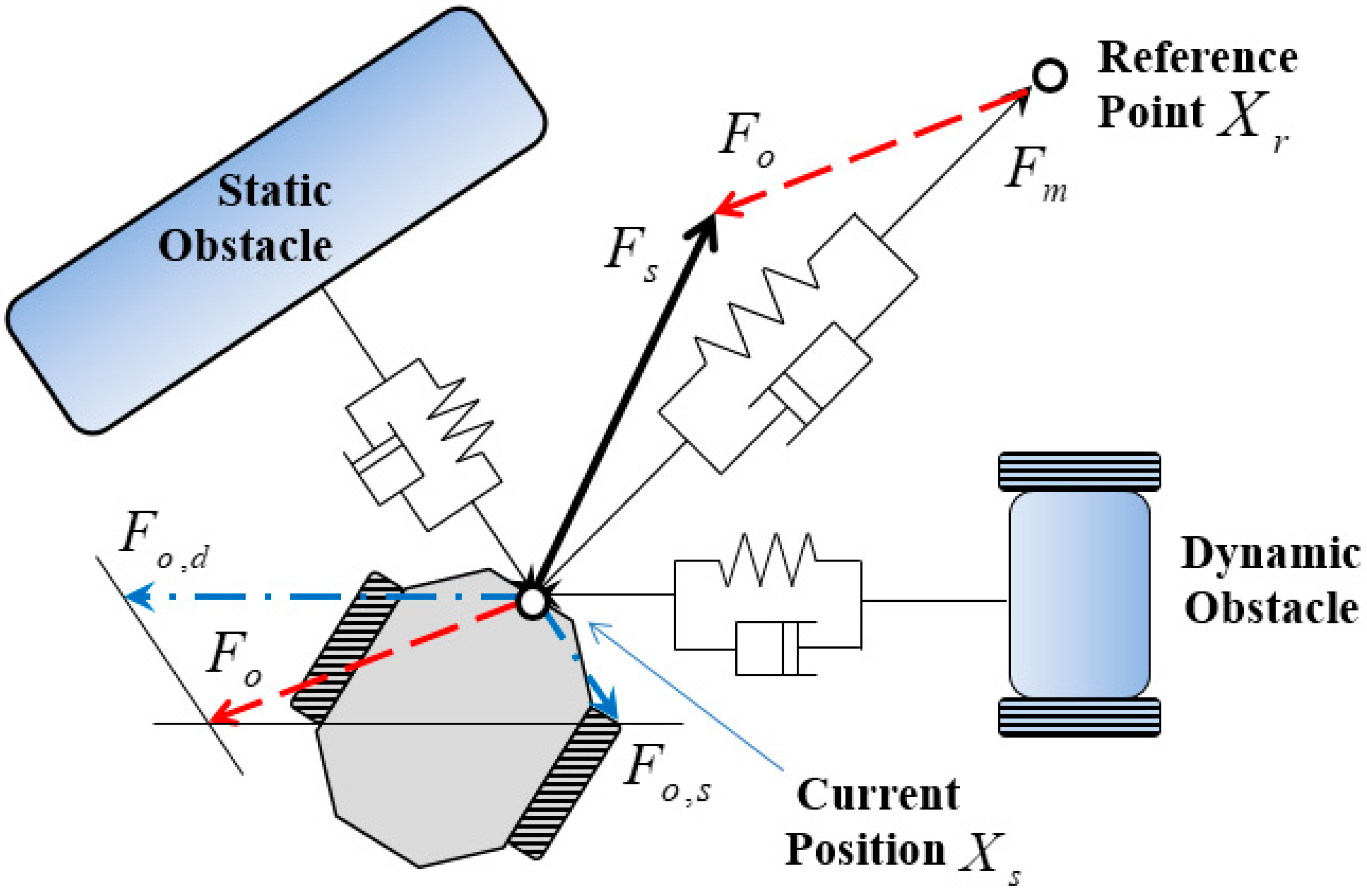
The relative distance and velocity between the mobile robot and an obstacle can be modeled as a spring and damper, respectively, which is called the virtual impedance. Using this virtual impedance, the acceleration for the mobile robot to avoid the obstacle, , can be defined.
From the virtual impedance model illustrated in
Figure 5, the motion equation of the mobile robot can be obtained as follows:
where
represents the attraction force to the target point,
;
represents the mass of the mobile robot;
and
represent the velocity and acceleration of the mobile robot, respectively;
and
are the repulsive force against the static and dynamic obstacles, respectively; and
and
represent the number of static and dynamic obstacles, respectively.
The addition of the three forces,
,
, and
, guides the mobile robot to the target while avoiding the obstacles. The forces are described in detail as follows:
where
,
, and
Note that and represent the position of the static and dynamics obstacles, respectively.
The variables in Equation (18) are summarized in
Table 3.
The repulsive force
can be represented using the obtained collision vector
with respect to the world frame as follows:
where
is a spring coefficient,
is a damping coefficient,
, and
represents the safety margin for avoiding the collision. These repulsive forces are generated regardless of the types of obstacles, and all the repulsive forces are added together.
For the static obstacle, the conventional virtual impedance algorithm is effective. On the other hand, when there are multiple obstacles, the mobile robot is jammed and cannot navigate farther. In addition, the sudden repulsive force against the moving obstacle causes unstable velocity changes in the mobile robot so that the mobile robot vibrates on the path or deviates from the path.
3.3. Active Virtual Impedance Algorithm
A new active virtual impedance algorithm is proposed to overcome the disadvantages of the conventional virtual impedance method that generates attractive and repulsive forces proportional to the distance and relative velocities with respect to the target and obstacle. Because the collision possibility increases abruptly when the obstacle approaches the mobile robot with a high relative velocity, a new nonlinear active virtual impedance was defined to incorporate the situations as follows:
where
and
and
are constants for repulsive forces;
and
determine the nonlinearities dynamically; and
is the maximum relative velocity of the obstacles, i.e.,
. This new nonlinear virtual impedance can be applicable for both static and dynamic obstacles.
Figure 6 shows the repulsive forces as a function of the distance and velocity against an obstacle as it is represented in Equation (19-a). As shown in
Figure 6a, the repulsive force by
against an obstacle is not zero, even for the obstacle farther than
. On the other hand, the repulsive force against the velocity is considered effective below,
, as shown in
Figure 6b. Note that when the relative velocity to the obstacle is larger than,
, the obstacle can mostly pass by the mobile robot safely. Using Equation (19-b), the virtual repulsive force,
can be represented as follows:
In conventional virtual impedance, the repulsive force is increased linearly with decreasing distance to the obstacle within a certain range. On the other hand, in this active virtual impedance algorithm, the repulsive forces are increased nonlinearly without a bound, as shown in
Figure 6. The advantage of this method is that a repulsive force is generated against a long-distance object to push away the mobile robot from the obstacle smoothly. This prevents the mobile robot from slipping caused by the abrupt change in direction and velocity.
To compare the distance and velocity factor, conventional virtual impedance holds that the repulsive force varies linearly in the positive or negative direction for the impact vector. Active virtual impedance determines the nonlinear form of the repulsive force in the exponential term. By multiplying the magnitude of the collision vector, the repulsive force cannot generate when the collision vector is zero or
. Consequently, the constraints of conventional and active virtual impedance differ, as shown in
Table 4.
In active virtual impedance, and values can be selected by comparison with and . In the case of , the magnitude get smaller and the total repulsive force gets smaller with movement to the left. when , to develop sufficient magnitude for the repulsive force, the magnitude of collision vector must be , and the magnitude of the repulsive force should be ; in the case of , the same is true.
At this point,
and
can be defined as follows:
5. Experiments and Discussions
In order to evaluate the performance of the model, the following three situations were tested. The experiment was carried out indoors with no concave or convex irregularities on the floor. In each experiment, spring and damper constants were selected through simulation to determine the attractive force of the sound source. The settings were and .
5.1. Experiment 1: Sound Source Tracking in Real Time
First of all, the sound source tracking performance of the mobile robot was checked in a 7.0 m 7.0 m obstacle-free space.
Figure 11 shows the sound source tracking operations of the mobile robot, which follows the moving sound source by detecting the distance and angle to the sound source using a microphone array. The tracking performance shows that the distance and angle can be estimated properly using the microphone array for the sound source tracking robot.
5.2. Experiment 2: Avoidance of Multiple Static Obstacles
The active virtual impedance algorithm was applied to mobile robot navigation under a static obstacle environment, as shown in
Figure 12, in which two obstacles were located in the path to the goal position.
Figure 13 compares the experimental trajectories using the conventional virtual impedance algorithm and the new active virtual impedance algorithm. For the conventional algorithm, the threshold value,
, to detect the obstacle was selected as 800 mm, and for the active virtual impedance algorithm, the maximum approaching velocity of the mobile robot,
, was selected as 600 mm/s.
As shown in
Figure 13, the trajectory of the mobile robot using the active virtual impedance algorithm was smoother than that using the conventional algorithm. This is the effect of the active virtual impedance, which detects long-distance obstacles and gradually changes the trajectory of the mobile robot earlier. Using this smooth trajectory, the mobile robot can reduce slippage on its path, i.e., it can increase the trajectory accurately during multiple obstacles avoidance.
5.3. Experiment 3: Avoidance of Dynamic Obstacles
The active virtual impedance algorithm was applied to dynamic obstacle avoidance for single and multiple obstacles.
Figure 14 shows the experimental environment of dynamic obstacle avoidance. The space was 6.0 m wide and 8.0 m long. The sound source was moving with a velocity of 300 mm/s, and
was set as 720 mm/s, which is the same as the maximum velocity of the mobile robot. Notice that the moving sound robot carried the sound source on the top of the robot.
Figure 15 shows the experimental results of the dynamic obstacle avoidance. As demonstrated in the sequence, the mobile robot successfully followed the sound source while avoiding the moving obstacle. As shown in
Figure 15c, the mobile robot collided with the obstacle when the conventional virtual impedance algorithm was utilized to avoid a collision. However, a strong repulsive force was generated by the active virtual impedance to avoid the collision.
Figure 15d illustrates the successful tracking of the sound source by the mobile robot while avoiding the two moving obstacles.
Figure 16 shows the experimental results of multiple dynamic obstacle avoidance. As demonstrated in the sequence, the mobile robot successfully followed the sound source while avoiding the two moving obstacles. As shown in
Figure 16b, the mobile robot moved downward quickly by using the repulsive force against the obstacle to avoid the collisions effectively. When the conventional virtual impedance algorithm was applied to this experiment, collisions occurred, as shown in
Figure 16c, because the impedance could not be adjusted properly for obstacle avoidance.
Figure 17 shows the experimental environment of multiple dynamic obstacle avoidance. The space was 6.0 m wide and 8.0 m long. The sound source was moving with a velocity of 300 mm/s, and
was set as 720 mm/s, which was the same as the maximum velocity of the mobile robot.
6. Conclusions
This paper proposed an active virtual impedance algorithm for obstacle avoidance and for following sound sources in real time using a mobile robot. The active virtual impedance algorithm changes the coefficients of the damper and spring dynamically depending on the possibility of collision with the obstacle, which makes the avoidance of the obstacle more efficient than when using the conventional virtual impedance algorithm. Before the mobile robot reaches obstacles, the motion trajectory of the mobile robot needs to be modified to prevent abrupt changes in the path, which may cause slippage of the mobile robot. The accuracy of the robot’s trajectory was demonstrated through real experiments. A microphone array was used to detect the location of the sound source, which is also a critical factor for successful sound source tracking. When there are omnidirectional dynamic obstacles in the working environment, three more ultrasonic sensors are necessary for the backside of the mobile robot to avoid collisions using an efficient algorithm, which will be the subject of a future study.


