1. Introduction
During the international conference on climate changes (COP21) in 2015, the 196 parties attending the conference in Paris highlighted the need for reducing greenhouse gas emissions [
1]. Urbanization is largely energy-intensive as reported by the United Nations habitat division, and cities consume about 75% of the global primary energy supply and are responsible for about 50–60% of the world’s total greenhouse gas emissions [
2]. Particular attention has been devoted to devising innovative strategies for both monitoring and improving energy efficiency of building heating systems, due to the significant incidence (roughly 40%) of these systems in the overall energy consumption [
3].
To this aim, the trend is to convert or upgrade the Physical Systems (as heat-exchangers) with Cyber-Physical Systems (CPSs), connected devices exploiting the Internet of Things (IoT) paradigm to monitor the heating distribution networks (HDN) in urban environments. CPSs allow the gathering of energy consumption values for each building every few minutes. Thanks to this new emerging technology, the data-generation capability of energy applications (e.g., the heating systems) has increased at an unprecedented rate, to such an extent that energy-related data rapidly scales towards big data [
4,
5].
The analysis of these large collections has received increasing attention from different and cross-research communities, including energy, data-mining, databases, and statistics communities. Big data collections have great potential because interesting subsets of actionable knowledge, such as detailed patterns and models to characterize and predict energy consumption at different granularity levels [
6], can be discovered to support the decision-making process of different stakeholders (e.g., energy managers, energy analysts, consumers, building occupants). To this aim, cutting-edge systems should be designed to continuously monitor energy consumption of buildings in a smart city environment [
7] through CPSs and provide all stakeholders with the analytic tools required to effectively support the improvement of energy efficiency.
Among the critical issues to be faced, an aspect of paramount interest for HDNs is the accurate prediction of both (i) energy consumption and (ii) peak power demand during the heating cycle, specifically for each building.
Such prediction tasks are very complex to address due to the high variability of the power profiles of buildings characterized by different heating cycles (e.g., one, two, or three in a day). Each heating cycle includes two main operational phases: the OFF-line phase, when the power exchange is turned off, and the ON-line phase, when it is on. The ON-line phase consists of two alternative states, named the transient state and the steady state. A large exchange of power between the building and the HDN happens during the transient state, which interleaves a more constant, i.e., steady, power exchange state.
Results of such predictions can be used by energy managers to estimate in advance the overall energy demand of the day after. Furthermore, the fine-grained predictions, performed building by building, provide additional value for energy managers. Knowing in advance the power exchanged by each heating system, energy managers can devise proper strategies to satisfy their specific energy demand during the entire day. Furthermore, they can address a more accurate sizing of the HDN for each city district, providing a more reliable service.
The peak power demand typically occurs during some specific time slots for most buildings connected to the network. Therefore, correctly predicting the peak, even in (near-)real time, for each building allows the energy analysts to better estimate the overall peak value and to adopt suitable countermeasures, hence avoiding interruptions of the heating distribution. Overall, it is possible to define targeted strategies to reduce the energy consumption during the critical time slots of the energy peak demand. An early knowledge of the future peak demand enables HDNs to adopt mitigation strategies, such as (i) deploying additional co-generators (e.g., gas boilers) to provide the necessary extra energy, (ii) advertising rewards in response of virtuous behaviors to increase people awareness and (iii) engage consumers to pursue power-saving behaviors. For example, a simple reward strategy might be discounting the bill when the customer shifts (anticipating or postponing) the starting of the heating cycle to re-balance the peak demand of the network.
This paper presents PHi-CiB (Predicting Heating Consumption in Buildings), a full-stack scalable engine addressing various services for energy management systems, from system modeling to energy data collection, integration, storage, and analysis. PHi-CiB gathers and integrates physical measurements collected through hardware entities (e.g., IoT devices) with third-parties information provided by software entities (e.g., web services). To address a wider set of analyses, both static (e.g., features describing some time invariant properties of the data source) and dynamic (e.g., monitored measures usually collected roughly every few minutes) data are integrated, hence creating richer data collections to be mined. In this study, the PHi-CiB engine has been tailored to predict future power consumption of the heating cycles for each building in an HDN. Fine-grained power consumption data have been integrated with the most common meteorological indicators (such as air temperature, relative humidity, cumulated precipitations and precipitation rate, wind speed, and atmospheric pressure) collected through weather stations distributed throughout the city and provided by third-party open-data services.
To deal with the high variability and mixed trend of the power profiles of different buildings, and to achieve accurate predictions, PHi-CiB exploits a three-step pipeline model. First, the (i) Status and Outlier Detection (SOD) algorithm automatically identifies the operational phases of the heating cycle of a building. Given a power measurement in a time instant, the SOD algorithm labels the current operation phase as OFF-phase or ON-phase, and this latter case is further categorized as transient or steady state. Then, the (ii) Peak Detection (PD) algorithm predicts the peak power value in the transient state, while the (iii) Power Prediction (PP) algorithm predicts the average power profile in both the transient and steady states.
PHi-CiB’s current implementation runs on Apache Spark [
8] and exploits the NoSQL distributed database MongoDB [
9] as data repository, hence supporting parallel and scalable processing and analytics tasks. As a case study,
PHi-CiB has been thoroughly evaluated on energy-related data collected in a real-world system in a major Italian city, where a large portion of residential buildings are served by the HDN. Experimental results show the effectiveness of
PHi-CiB to accurately predict heating power exchange levels with a limited prediction error, and its optimal scalability. Currently, our work is validated on prediction performance. To this aim, we do not address the evaluation of security and adequacy indices of the system.
This paper is organized as follows.
Section 2 reviews relevant literature solutions.
Section 3 introduces an overview of the
PHi-CiB engine, while
Section 4 and
Section 5 describe its main layers.
Section 6 presents the proposed analytics methodology to predict the average power levels of the heating systems, then
Section 7 discusses the experimental results obtained on real data. Finally,
Section 8 discusses the impacts of the proposed methodology in both the industrial and academic perspectives, while
Section 9 draws the conclusions and presents some future developments of this work.
2. Related Work
Many research efforts have been carried out for designing and developing systems to provide novel and scalable analytics services based on big data and IoT technologies.
2.1. General-Purpose and Data-Driven Solutions
Different general-purpose approaches have been proposed, most of them targeting a wide spectrum of applications, e.g., within the smart-city context, or focusing on the exploitation of data-oriented large-scale technologies, e.g., NoSQL databases. In [
10], authors present an architecture for big data analysis in smart cities. Its main characteristics are the scalability and the flexibility, provided by its hierarchical structure and a distributed design based on fog computing. Other general-purpose approaches propose data management engines based on NoSQL databases [
11] or pervasive monitoring IoT-based systems [
12,
13].
The authors in [
14] propose a smart-city data management framework that can share/publish data with different sensitivity levels. The framework takes advantage of big data technology for data storage and processing, provides a streamline processing workflow for data quality checking and data anonymization, and proposes a regression-based quality checking model according to a data-driven feature extraction approach. The system architecture of the proposed framework is developed with four layers: (i) Data-Source Layer, collecting data from the field; (ii) Data-Staging Layer, temporarily saving the data from different source systems; (iii) Data-Transformation Layer, which is in charge of cleansing the data, combing data from multiple-sources, removing duplicates and executing the anonymization step; (iv) the Data-Storage, Publishing, and Retrieval Layer.
In [
15], authors investigate different big data services using a Hadoop-based large-scale distribution-system platform. They point out that most of the services they analyzed aim to increase the energy efficiency and to decrease the cost in heat consumption and maintenance.
Other approaches are focused on providing specific technological and algorithmic contributions, such as clustering techniques [
16,
17], simulator engines [
18], and association rule mining [
19]. Such works exploit data-mining techniques, often based on both supervised (e.g., classification and prediction models) and unsupervised learning (e.g., clustering), hence proposing hybrid models. They can take advantage of the labeled historical data when the training labels are provided. However, they also tackle the problem when no labels are present, by exploiting powerful exploratory techniques such as rule mining. Similar combinations of such techniques have also been successfully applied in other domains, e.g., for network data characterization [
20,
21].
2.2. Energy Domain Applications
In recent years, a strong research effort have been devoted in developing solutions tailored to the heating systems of buildings specifically addressing the following contributions: (i) data management platforms; (ii) characterization of energy consumption and environmental impacts, and (iii) data-mining, modeling, and forecasting of energy consumption.
In the field of data management, Ferreira et al. [
22] proposes a platform for aggregating useful information from several sources, using a service-based approach. The data are collected on a time-based fashion: daily schedules, deadlines defined in the academic calendar, opening hours for administrative services. Sustainability-related data such as climate, energy, water, and building occupancy are also collected. Interested users can subscribe to specifics topics of a central aggregator service. Such service also allows collection of data directly from users that are not available in any other way. The authors conclude that the data collected by the platform can be used to develop a calibrated model for a preventive midterm managing tool enabling energy saving.
In [
23], authors present the design and implementation of an event-driven service-oriented middleware for energy efficiency in buildings and public spaces. The presented middleware aims to provide a tool for developing user-centric applications. Furthermore, the work presents a complete and real deployment in historical buildings.
Brundu et al. [
24] present a distributed IoT platform able to collect, process, and analyze energy consumption data and structural features of systems and buildings in a district. Their solution integrates heterogeneous data sources, such as data from building information models, system information models and Geographic Information Systems (GIS) that are correlated and enriched with historical and (near-) real-time collection of data from heterogeneous IoT devices. The authors tested the software infrastructure in a real-world case study with hundreds of devices connected to monitor and manage the HDN.
In the field of the characterization of energy consumption, Dall’O et al. [
25] present a methodology based on GIS data that estimates energy savings in residential buildings after retrofit. In their methodology, authors exploit a simple linear regression among primary energy use and the shape factor with respect to the construction years. Such methodology has been applied to five municipality of the Milan province, north-west of Italy. In [
26], a statistical bottom-up model to estimate energy use in buildings has been proposed. The authors consider space heating, electricity, and domestic hot water. Mastrucci et al. [
27] propose an Ordinary Least-Squares Method for statistically estimating the heating energy demand and indoor thermal comfort of building stocks in cities by following a bottom-up approach.
Ma et al. [
28] proposes a framework that integrates GIS and big data technology for estimating building energy consumption at urban level. The proposed solution has been applied to 3640 buildings in New York city for testing and validation. The study does not focus on the prediction of load profiles but on the classification of energy intensity consumption in buildings.
In [
29], authors present a Bayesian Statistical Inference method for expressing energy efficiency performance of residential building stocks. The aim of the model is to provide local authorities with a decision-making service for planning refurbishment interventions.
Moghadam et al. [
30] present a bottom-up statistical model based on GIS. The model aims at estimating energy consumption of space heating in residential building stocks. They exploit 2D/3D maps and Multiple Linear Regression to provide geographically referenced information for each single dwelling. The objective is to identify correlations and to assess the demand-side consumption at urban scale. This solution has been tested on 3600 buildings belonging to the municipality of Settimo Torinese, north-west of Italy.
Domínguez et al. [
31] presents a dimensional reduction method based on self-organizing maps to analyze building heating systems. It is used to monitor all the system variables and to establish correlations between temporal production and distribution variables. Furthermore, authors propose a method to analyze the daily heating consumption based on the t-SNE dimensional reduction technique. Both solutions have been tested in a real heating system in a building in the campus of the University of León. From their analysis and thanks to this solution, authors were able to find some faults in system elements and abnormal behaviors in circuits.
EDEN [
32] and ESA [
33], our previous works, are two big data-oriented systems exploiting scalable technologies to compute a variety of key performance indicators (KPIs). Basic KPIs in [
32] (i.e., energy consumption per unit of volume during specific outdoor conditions) and advanced KPIs in [
33] (i.e., inter/intra-building KPIs based on the energy signature estimating the total heat loss coefficient of a building) have been proposed to characterize the energy consumption of buildings connected to HDN.
In the field of data-mining applied to model and forecast energy consumption, Liu et al. [
34] propose a top-down black-box-based behavioral modeling technique. The authors present a subspace identification method to obtain the control-friendly state space models for building thermal behaviors. This solution studies the relationship between model order and model prediction accuracy. Furthermore, it uses a cross-validation technique to find the optimal order to avoid overfitting and underfitting.
Ghosh et al. [
35] present a grey-box model to identify building thermal dynamics. The authors apply latent force models augmenting the simple grey-box thermal model with a time-varying residual. Such residual attempts to model the latent forces in a building that can i) influence the evolution of the internal temperature trends and ii) cause alterations in the thermal dynamics.
In [
36], authors present a method for predicting energy consumption in buildings. This solution is composed by four different layers, namely: (i) data acquisition; (ii) pre-processing; (iii) prediction and (iv) performance evaluation. Data have been collected only from four real multi-storied residential buildings. First, collected data are pre-processed to remove outliers. Then, three different machine learning algorithms are tested based on: (i) deep extreme learning machine, (ii) adaptive neuro-fuzzy inference, and (iii) artificial neural networks.
In [
37], authors propose a solution for thermal load forecasting that combines different data-driven methods based on: (i) linear regression, (ii) artificial neural network, (iii) support vector machines, and (iv) extra tree regressors. This solution predicts the hourly thermal load of the next day by combining weighted predictions of the four algorithms. Input variables include day of the week, hour of the day, and forecast outdoor temperature. The performance assessment of the algorithms is carried out with data about thermal load of ten residential buildings located in Rottne (Sweden) over a time horizon of 27 months, by comparing the Mean Absolute Percentage Error (MAPE). The approach based on artificial neural network with full features gives best performance (11.56%), while the compound prediction has a MAPE of 11.95%.
Ahmad et al. [
38] propose an accurate model to predict the energy level in districts for medium- and long-terms (i.e., 1-month and 1-year, respectively). This solution exploits three different machine learning techniques based on: (i) artificial neural network with nonlinear autoregressive exogenous multi-variable inputs; (ii) multivariate linear regression model, and (iii) adaptive boosting model.
In [
39], authors propose a comparison of two data-driven models for thermal load forecasting. The first model is based on support vector machines exploiting a radial basis function and a polynomial kernel. The second consists of two Nonlinear Autoregressive Exogenous Recurrent Neural Networks (NARX) with different depths. For training and testing the two algorithms, authors used an historical data set with monthly loads from a non-residential district in Germany. From their results, authors demonstrated that both NARXs have a higher accuracy than the model based on support vector machines.
In [
40], data-mining techniques are applied to analyze two substations in HDN located in Changchun, China. The authors tested their solution on a data set reporting information from two different substations. They conclude that both substations exhibit six operating states over the entire heating season. These states represent the variation of heat supply. The duration of the heating time is increased or decreased to meet the variation of consumer heat demand during each heating period. Thus, identifying these operating states is not trivial due to this time dependency. This is also a limitation of this solution, as pointed out by the authors. To overcome this issue, our methodology identifies the operating states by considering only associations between attributes without time dependency.
Finally, Suryanarayana et al. [
41] investigate the performance of three different linear models to forecast energy consumption: (i) linear, (ii) ridge, and (iii) lasso regression. The authors compare such methods with another solution based on deep-learning techniques. The study is conducted over two different HDN serving two cities in Sweden, Rottne and Karlshamn, respectively. They compare these methodologies in predicting the day-head overall heating consumption and not the single building energy demand. The authors conclude that for the case study in Rottne the model based on deep-learning is the best. Meanwhile, for the case study in Kaelshamn, they could not choose the best model since the performances are comparable.
2.3. Comparison and Contributions of the Current Work
Presented solutions in energy-related analysis have limited or no integration of IoT devices and metering infrastructure or do not provide forecasting and characterization algorithms, hence reducing the impact on emerging smart-city applications. In particular the works [
22,
23,
24] propose only platforms or middlewares for integrating heterogeneous energy-related data sources for energy management purpose. None of such works provides energy characterizations, prediction, or analytic tools. Furthermore, in the works [
25,
26,
27,
28,
29,
30], solutions for the energy characterization of buildings and potential savings from possible retrofits are presented. However, such works lack in the integration of real data and none of the proposed methodologies integrates IoT devices and metering infrastructure, hence limiting the applicability in future smart cities for both planning and operational phases. Finally, the works [
31,
34,
35,
36,
37,
38,
39,
40,
41] propose either clustering [
41], or fault location [
31], or prediction techniques [
34,
35,
36,
37,
38,
39,
40] at the building [
31,
34,
35,
36,
37] or at the district scale [
38,
39,
40,
41]. Such solutions do not provide an integrated and distributed system able to collect a large volume of energy-related data and efficiently compute both characterization and forecasting of energy consumption, applied in a real-world use-case scenario. In particular, for the prediction of the load profile none of the state-of-the-art solutions provides a day-head prediction with a fine-grained 5-min resolution.
In the proposed approach, the energy forecast is given by combining three algorithms, namely: (i) Status and Outlier Detection exploiting an exponential moving average, (ii) Peak Detection applying a Multivariate Adaptive Regression Spline, (iii) PP based on linear regression with stochastic gradient descent.
Furthermore, differently from the previous research works, this paper proposes an overall architecture exploiting different big data technologies to support the full life-cycle of energy-related data.
Our previous work [
32,
33] has a completely different target and analytic approach, and a different architecture (the only similarity lies in the data warehouse design and the data types). Furthermore, the methodologies proposed in [
32,
33] exploit the Map-Reduce paradigm, while this work takes advantage of the Apache Spark implementation and a MongoDB [
9] data repository, supporting parallel and scalable processing and analytic tasks.
3. The PHi-CiB Engine
PHi-CiB is a scalable full-stack distributed engine addressing a variety of tasks for energy management systems.
Figure 1 shows the overall architecture of the
PHi-CiB system. Since
PHi-CiB has been designed for the collection, integration, modeling, storage, and analysis of energy-related data, it consists of a four-layered architecture with: (i) a
Data-Source Layer; (ii) a
Middleware Layer; (iii) a
Storage and Data Analysis Layer, and (iv) an
Application Layer, briefly presented here and then detailed in the following sections.
The PHi-CiB architecture can be easily tailored to fit different indoor or outdoor monitoring contexts (e.g., electric cooling), however, in this study, we focus on a specific instance of PHi-CiB tailored to predict power consumption of the heating cycles of buildings in an HDN.
The Data-Source Layer includes smart meters and web services that continuously provide data of interest to the PHi-CiB system. Such data sources typically provide measurements roughly every 5 min. The Middleware Layer enables the interoperability across these heterogeneous data sources, by creating a peer-to-peer network in which the communication between peers is trusted and encrypted. Collected data are managed by the Storage and Analytics Layer which oversees integrating data and storing them into a non-relational scalable database to effectively support different complex analytics tasks. A variety of algorithms have been designed, developed, or integrated in PHi-CiB to support data-mining operations and analytics. At the end, the Application Layer exploits the knowledge items discovered through the data analysis process to provide useful feedbacks to the different interested users and stakeholders, and to suggest ready-to-implement energy-efficient strategies.
4. Data Collection
In a smart-city scenario, one of the main issues concerns the coexistence of several heterogeneous technologies. Moreover, future smart-city systems will deal with IoT [
42] environments, where multiple actors need to access transparently IoT resources and services. Hence, the lack of interoperability among heterogeneous technologies must be addressed. To cope with these issues, we developed a distributed software infrastructure that exploits a middleware approach to integrate different IoT devices and technologies. The aim is providing many services for collecting and managing energy-related data.
PHi-CiB adopts the open-source LinkSmart middleware [
43] and extends its features to fulfill the requirements for a smart-city context. Indeed, an IoT middleware for a smart city needs (i) to be highly available, (ii) to scale up rapidly, and (iii) to provide a uniform interface to all deployed technologies [
44,
45].
4.1. Data-Source Layer
The
Data-source Layer is the lowest layer in
PHi-CiB (see
Figure 1). It can include different kinds of hardware and software entities that continuously provide various data types of interest to
PHi-CiB.
Hardware entities correspond to
IoT devices measuring physical quantities. Instead,
software entities are
software services exposing to external clients physical measures collected from third-parties. They allow the acquisition of data values complementary to those collected through hardware entities that contribute in the overall characterization of the context under analysis. Web services are an example of software entities that expose interfaces over the Internet allowing clients to send requests and get data using HTTP as transport protocol.
Nevertheless, any data source can be integrated in the Data-Source Layer, in this study we focused on a layer composed as follows. (i) A network of smart meters as IoT devices (hardware entities) located in buildings within an HDN to measure building thermal energy values. A single smart meter is in each building. (ii) web services (software entities) to monitor surrounding conditions when measurements of thermal energy take place. Different web services can be considered to enrich measurements collected through the smart meters. We selected those exposing meteorological data due to the well-assessed strong correlation between climate conditions and thermal energy consumption.
Each data source in the layer provides the following two types of data: (a) dynamic data as monitored measures usually collected roughly every few minutes and potentially exhibiting highly variable values; and (b) static data as features describing some time invariant properties of the data source (as the location of the monitoring nodes).
In the
PHi-CiB instance considered in this study,
dynamic data include measures on
building thermal energy and
climate conditions collected roughly every 5 min, even if different and variable resolutions can be considered. Thus, a large volume of energy-related data is continuously acquired for each building. Smart meters installed in buildings provide fine-grained data related to building thermal energy (as instantaneous power, cumulative energy consumption, water flow, and corresponding temperatures). Meteorological web services (e.g., Weather Underground [
46] considered in this study) provide different kinds of meteorological data as temperature, relative humidity, precipitation, wind direction, UV index, solar radiation, and atmospheric pressure. Such data are collected through several weather sensors deployed throughout the city.
For each monitoring node (building smart meter or weather sensor), static data report features characterizing the data source as its geographical location (longitude and latitude). Static data also include information characterizing buildings as the volume of each building where smart meters are located. This value is used to normalize energy and power values to allow comparison between buildings in terms of consumption per volume unit. When a new data source registers for inclusion in the Data-Source Layer, all related static data are acquired, and then stored in the PHi-CiB data repository.
Measurements collected from the hardware and software entities are also enriched in
PHi-CiB with additional
spatio-temporal information useful to describe the spatial and temporal distribution of the acquired values (e.g., the spatio-temporal distribution of thermal energy consumption). To this aim, the Data-Source Layer also includes additional
contextual data sources such as web services exposing topological data (e.g., Municipality open-data portals [
47]) or calendar data. More specifically, the geo-coordinates (longitude and latitude) of each monitoring node are mapped to the corresponding neighborhood and city district including that neighborhood. Meanwhile, the georeferenced location of nodes is given in the hardware/software entities, both the neighborhood and district names corresponding to the georeferenced location have been added as additional contextual features. They have been retrieved from contextual data sources. Moreover, each measurement time is associated with different blends of time spans as daily time slot (e.g., morning, afternoon, evening, or night), week day, holiday or working day, month, 2-months, or 6-months’ time periods.
To effectively support the interoperability across heterogeneous IoT devices possibly included in the Data-Source Layer,
PHi-CiB exploits the concept of
Device Connector (see
Figure 1). It is a middleware-based component that abstracts a given technology and translates its functionalities into web services. The Device Connector enables the communication among heterogeneous devices by allowing developers in exploiting each low-level technology transparently. Thus, it works as a bridge between the Middleware Layer and the underlying technologies or devices in the Data-Source Layer.
4.2. Middleware Layer
The
Middleware Layer (see
Figure 1) is in charge of providing features to discover available resources and services in the Data-Source Layer. It creates a network among different entities that can exchange information exploiting two communication paradigms: (i) request/response based on REST [
48] and (ii) publish/subscribe [
49] based on MQTT protocol [
50]. Such features are key characteristics of a software infrastructure dealing with IoT devices. The Middleware Layer includes four software components described below.
The
Message Broker allows the communication among different entities (both hardware and software) through the publish/subscribe paradigm. This approach supports the development of loosely coupled event-based systems. Indeed, it removes explicit dependencies between interacting entities (i.e., producer and consumer of the information), thus each entity in the middleware network can publish data and other subscribers can receive it independently. This increases the scalability of the whole system [
51].
PHi-CiB adopts the MQTT communication protocol [
50] and delivers data to subscribers as soon as they are measured and published (the delay is negligible).
The Resource Catalog registers and provides a list of IoT devices and resources available into the middleware network. It exposes JSON-based REST API to automatically access and manage such information. For instance, Device Connectors register their devices and resources, while other middleware-based entities discover such devices and their access protocols.
The Service Catalog provides information about available services in the middleware network exposing a JSON-based REST API. It is used by middleware-based entities to discover available services in the network. For instance, it provides the end-points of services such as Resource Catalog and Message Broker.
The Security Manager provides features to enable a secure communication among entities in the middleware network. Indeed, it is in charge of authenticating and granting accesses to applications and other middleware-based components. Hence, malicious actors cannot call services in the middleware network and cannot receive any kind of data.
5. Data Management and Analytics
This section presents the Data-Storage and Analysis Layer of PHi-CiB that provides different services to address data management and storage as well as analytics tasks.
5.1. Data Integration Layer
The aim of the current layer is to integrate information from heterogeneous data sources, hence gathering a rich and exploitable data collection, used for feeding the subsequent data analysis phase. Each source can either proactively send its data to the Message Broker using the MQTT protocol, data that are automatically forwarded to the Message Subscriber; or expose a REST API enabling the Contextual Enrichment Agent to collect the required information. For each data source, monitoring nodes are typically deployed in different locations of the city and they may adopt different sampling periods. Thus, a proper strategy should be devised to address the spatio-temporal integration of the acquired measurements. The Synchronizer module manages the alignment of weather data and power data, both in time and in space, so that given a power consumption value from a building, it can be associated with a specific weather condition at the right time and in the corresponding location.
Furthermore, in PHi-CiB power measurements collected through smart meters are enriched with weather data of external third-party web services. Specifically, each power measure collected for a building is associated with a set of weather measures (e.g., temperature, humidity, and pressure) that describe the climate condition when the power measure was collected. Each weather measure (e.g., temperature) is calculated as the weighted mean value of the corresponding measures acquired from N weather stations located near the building. A weight is associated with each weather station based on its proximity to the building. It expresses the relevance of the measure provided by the weather station. The weight is higher for stations closer to the building since they provide a more accurate value on the climate condition at the building proximity. For each weather station, only the closest weather measures in time are considered.
5.2. Data-Storage Layer
Due to the different kinds of collected data and to easily manage more data types in the future,
PHi-CiB exploits a document-oriented distributed data repository providing rich queries, full indexing, data replication, horizontal scalability, and a flexible aggregation framework. Integrated and enriched data are formatted as JSON documents and stored in a NoSQL repository (i.e., MongoDB [
9]), which is used as
Historical Data-Store. This collection of historical data is then exploited to create models of the energy consumption for the buildings and for the (near-) real-time data analysis, including building PP.
According to the objectives of the data analysis tasks described in
Section 5.3, we evaluated as optimal choice the adoption of the data processing framework Apache Spark [
8] upon MongoDB data repository (see
Section 7.2). MongoDB stores data across different nodes (called shards), thus supporting parallel processing by Spark. This distributed architecture provides higher levels of redundancy and availability, which are fundamental when operating in (near-)real time, and to scale and satisfy the demand of a higher number of read and write operations. Since both Spark and MongoDB adopt a document-oriented data model, they exchange data in a seamless way by making use of the JSON serialization format. This way, Spark jobs are executed directly against the Resilient Distributed Datasets created automatically from the MongoDB data repository, without any intermediate data-transformation process. Moreover, due to the real-time nature of the data analysis, input data sets vary rapidly in time. To improve the performance of the several queries to be executed, MongoDB rich-indexing functionalities are exploited in Spark, like secondary indexes and geospatial indexes that allow efficient filtering of data according to the geospatial coordinates of buildings and nearby weather stations.
5.3. Data Analysis Layer
In this study, the PHi-CiB engine is used to predict the fine-grained power-level values during the heating cycle of buildings.
The data prediction process is structured into three main blocks: (i) data-stream processing to support (near-) real-time data analysis, (ii) prediction analysis, and (iii) prediction validation. The main functionalities of the three blocks are briefly presented below and detailed in
Section 6.
Data-stream processing. Since thermal energy consumption is monitored roughly every 5 min in the HDN, a large volume of energy-related data is continuously collected from each building. To efficiently and effectively analyze such large data collection, the PHi-CiB engine performs the power-level prediction task through the data-stream analysis over a sliding time window, separately for each building. Every time a new measure of power level is collected, one single time window, sliding forward over the data stream of energy-related data, is considered for the prediction task. This window content contains the recent past energy-related data for the building heating system, corresponding to thermal power levels, along with data about weather conditions related in space and time to those power measures. Consequently, it allows predicting the upcoming value for the building in the near future.
Prediction analysis. This block entails to predict the average future power levels for each building. A prediction model is built for each building separately by considering the energy-related data in the current sliding time window. The building model is then exploited for forecasting the average power level at a given time instant in the near future.
Before presenting the proposed data analytics model, we recall how the heating cycle of buildings works. In an HDN, the heating cycle of a building includes two main operational phases: the OFF-line phase, when the power exchange is turned off, and the ON-line phase, when the power exchange is on. The ON-line phase is then further structured in the alternation of two sub-phases, named the transient state and the steady state. More in detail, a large exchange of power between building and HDN (transient state) interleaves a quasi-constant power exchange between building and HDN (steady state).
To deal with this mixed trend and achieve an accurate predicted value, we devised a prediction model composed of three contributions applied in cascade. First, the proposed approach allows the automatic identification of the operational phases described above. Then, it allows forecasting the power level locally at each phase. More specifically, (i) first the
Status and Outlier Detection algorithm automatically identifies the operational phases of the heating cycle of a building (
Section 6.1). Given a power measurement in a time instant, the SOD algorithm labels the current operation phase as OFF-phase or ON-phase, and this latter case is further categorized as transient or steady state. (ii) Then, the
Peak Detection algorithm predicts the peak power value in the transient state (
Section 6.2), while (iii) the
PP algorithm predicts the average power profile in the transient state and in the steady state (
Section 6.3).
Prediction validation. This block measures the ability of the PHi-CiB engine to correctly predict the energy consumption values achievable by a building in an upcoming time instant. To this aim PHi-CiB integrates two metrics named Mean Absolute Percentage Error (MAPE) and Symmetric Mean Absolute Percentage Error (SMAPE). Every time a real power level value is received, their values are updated to include the prediction error for the new measure.
5.4. Data Flow to Support the Prediction Task
This section describes the data flow for power levels prediction by exploiting data coming from both IoT devices and third-party systems such as web services. IoT devices (i.e., smart meters) are deployed in buildings to monitor the status of the heat-exchangers. As shown in
Figure 2, they exploit the MQTT protocol [
50] to publish energy-related measures as messages with an associated topic. A message includes the power value measured on the heating system of a building, the identifier of the same building and the timestamp of the measurement. Messages are asynchronously collected by the
Message Broker, using the publish/subscribe mechanism, and distributed to all interested subscribers. Therefore, subscriber nodes are responsible for gathering data notifications about new power measures published by IoT devices to the
Message Broker.
In our scenario, among the subscribers there are the (near-) real-time algorithms, i.e., PP and SOD. Each algorithm independently receives energy-related data, sent by IoT devices, from the Message Broker and retrieves meteorological information from third-party web services through REST interfaces [
48]. Furthermore, the algorithms gather data from the
Building Model, included results from the PD algorithm, which works with already collected historical data. Finally, the results of (near-) real-time algorithms are stored into the MongoDB
Historical Data-Store.
The PP algorithm uses the energy-related measures received from the Message Broker to develop the building model for the prediction of future power values. Whenever a new power measure is available for a building, the PP algorithm updates the corresponding model, to use it for predicting the next power values. PP contextually exploits the received measures to calculate the errors of the predictions previously performed for that values, to validate the model. It computes the prediction error based on the expected power values according to the prediction model and the actual power value just received. After data have been processed, they are stored in the Historical Data-Store together with the produced outcomes.
6. Analytics Methodology
The purpose of our analytics methodology is to predict the future power profiles in the heating cycles of the building heating systems.
To achieve this objective, the
PHi-CiB engine integrates the three algorithms, named
Status and Outlier Detection,
Peak Detection, and
PP, introduced in
Section 5.3 and described in detail in this section.
All the algorithms elaborate building models based on, and trained with, a collection of historical data retrieved from the Historical Data-Store. Each algorithm defines an appropriate time window in the past from which data are taken for training. Considered data include power-level measurements, possibly coupled with weather data (for PD and PP). The adoption of the windowing approach allows considering only the recent past data, while excluding a lot of too old samples. Consequently, the training phase becomes faster, and the generated model fits the behavior of the heating system just during the selected period.
6.1. Status Detection
The SOD algorithm aims at automatically identifying the current operational phase for the building heating system. SOD also allows the smoothing of abnormal values of the instant power measurements potentially occurred in the steady state.
The operational phases of the heating cycle are the OFF-line and ON-line phases, with the latter characterized by the alternation of a transient and a steady state. The transient state is characterized by a rapid increase of power consumption. It usually occurs in the early morning when the heating is turned on. The steady state is characterized by a relatively constant power consumption, and typically occurs after a transient state. Each of the above operational phases is characterized by a different amount of power exchange between the building and the HDN. Specifically, the power exchange occurs only during the ON-line phase, while it is absent otherwise.
The SOD algorithm relies on these expected trends in the power exchange to detect the operational phase based on the measured instant power values. Specifically, SOD adopts the
Exponentially Weighted Moving Average (EWMA) to detect the dynamic transient of the heating cycle. Furthermore, possible abnormal variations in the steady state are smoothed by EWMA, similarly to noise filtering in a signal, as described in [
52].
First, SOD computes the exponential mean () and the corresponding standard deviation () values of the instant power over a sliding window with one-day size. The day preceding the current day is used for positioning the sliding window. This time period allows computing and over a significant number of power values, but sampled in time instants not too distant from the current time. Power values in the range represent the expected power exchange during the steady state for the considered building. This range of power values is used as a reference for the identification of the operational phases. When a new instant power measurement is acquired at time , SOD assigns a class label describing the current operational phase of the building heating system. The phase categorization process works as follows. The ON-line phase is detected when the instant power is different than zero (); otherwise the phase is identified as OFF-line. The steady-state label is assigned when the instant power is within the reference range of power values (i.e., () ≤ ≤ ()) for at least a minimum amount of time (transition threshold). Instead, the transient state is labeled when the instant power is out the reference range of power values ()) for more than the transition threshold.
For example,
Figure 3 plots the instant power measures monitored in one day for a building. The figure also reports the range
computed considering power values collected in the preceding day. Instead,
Figure 4 shows the status labels assigned by SOD when two consecutive days of power measurements are considered. The assigned labels are equal to 1 for the transient state, to 0.5 for the steady state, and to 0 for the OFF-line phase. To increase readability, the power value reported in the figure has been normalized to the maximum power value. In both days, the SOD algorithm identifies one transient phase (around 07:00), followed by one steady state.
The SOD algorithm also allows detection and removal of abnormal values in the instant power measurements occurred during the steady state. An abnormal value is an observation that lies outside the expected range of values. It may occur either when a measure does not fit the model under study or when an error in measurement occurs (e.g., caused by faulty sensors). SOD categorizes this abnormal value as an outlier. When the operational phase is the steady state, a single isolated power measure
is categorized as outlier if its value is out of the range characterizing the steady state, i.e.,
. For example,
Figure 4 shows an outlier detected during the steady state at around 3:00 p.m. in the second day of monitoring.
6.2. Peak Detection
The PD algorithm aims at (i) forecasting the peak power value in the transient state and (ii) identifying the peak power time instant, separately for each building.
The building heating cycle can have a single daily occurrence, or it can be repeated more times per day. Thus, the PD algorithm can be employed only once or more times to forecast the peak power value in each transient state. Through the evaluation of the heating cycle for a large collection of buildings (about 300 buildings), we identified three main building categories based on the number of interleaved heating cycles per day. These categories represent buildings that are daily characterized by a Single, Double or Triple Heating Cycle.
Figure 5 reports an example of the daily power profile for the three categories. Please note that consecutive heating cycles can show different peak power values in case of variation in the external temperature. The building internal temperature is affected by the values of the external temperature. When the external temperature decreases, the heating system reacts with a higher power exchange to keep the building internal temperature at the desired value of comfort. Thus, when the heating system turns on after an OFF-line phase with a lower external temperature, the heating cycle is characterized by a higher peak power value in the transient state.
To predict the peak power value in the transient state, the PD algorithm hypothesizes a relation between two quantities, named and . is the ratio between the peak power value in the transient state and the mean power value in the previous steady state. is the mean external temperature value in the previous steady state and OFF-line phase.
To properly model the relationship between the
and
values for any of the three classes of buildings, the PD algorithm relies on the
Multivariate Adaptive Regression Spline (MARS) [
53] approach. MARS is a step-wise linear regression for fitting variables in distinct intervals by connecting different splines with knots, thus it is suited to model a wide class of nonlinear relations between variables. PD exploits the modified version of the MARS model proposed in [
54] to predict the energy performance of buildings. PD learns a regression model for each building and for each peak using as training set the data collected in the past days.
and
represent respectively the dependent and independent variables of the regression. Since all the other quantities of
and
are known (from past data), the peak power value of the transient state appearing in
is the final target of the prediction.
For predicting the peak power value in the transient state of the first, second, and third heating cycles (named first, second and third peak value, respectively) in the target day, PD calculates the and values as described below. PD predicts the first peak value for all three building categories (Single, Double, and Triple Heating Cycle), while the second peak value for two categories (Double and Triple Heating Cycle) and the third peak value for a single category (Triple Heating Cycle).
To forecast the first peak value, and are computed as follows: is calculated as the mean external temperature value during the last steady state and OFF-line phase in the day preceding the target day; is the ratio between the first peak power value (to be forecast) and the mean power in the last steady state of the day preceding the target day.
To forecast the second peak value, is the mean external temperature value during the first steady state and OFF-line phase in the target day; is the ratio between the second peak value (to be forecast) and the mean power of the first steady state of the target day.
To forecast the third peak value, is the mean external temperature value during the second steady state and OFF-line phase in the target day; is the ratio between the third peak power value (to be forecast) and the mean power in the second steady state of the target day.
The PD algorithm also infers the instant at which the peak power will occur. To this aim, PD computes the mean time where the past peaks have occurred, by considering a sliding window of fixed size preceding the current instant of time.
6.3. Power Prediction with Multiple Regression
On the basis of the outcomes of the SOD and PD algorithms, the PP algorithm exploits the multiple version of the
Linear Regression with Stochastic Gradient Descent (LR-SGD) [
55] to predict the average power levels based on data from the Historical Data-Store.
PP defines a
building model based on a linear dependency between weather data and power level. PP relies on the assumption that the average power exchange for a building heating system at a given time instant is likely to be correlated with the surrounding weather conditions. Moreover, the average power levels are also likely to be temporally correlated with each other [
33].
PP trains a Multiple Linear Regression model for each building using historical data on weather conditions and power level. The training set is built using a fixed width sliding window mechanism, so the samples not older than a certain amount of time before the current time instant are included. For collecting samples, we assumed to split the window timeline in slots of the same duration (slot duration). Within a time slot, a single sample for each variable (power and weather parameters) is considered, computed as the mean value of the measures taken during the slot. Data sampling is performed for both training and test (i.e., future time slots) datasets.
The LR-SGD algorithm is characterized by a set of input features expressed through a n-dimensional vector x = [] and a target variable representing the objective of the prediction. The LR-SGD algorithm builds a hypothesis function x) so that given an input vector x, function x) provides a good estimation of the value of y. In our study, features in x correspond to the weather variables (air temperature, humidity, precipitations, wind speed, pressure), while y is the power level. Since power consumption and meteorological values differ in scale and measurement unit, data have been normalized. To preserve the original data distribution without affecting the prediction accuracy, the Z-Score standardization technique has been adopted.
The PP algorithm is structured into two phases: (i) building model learning, considering a collection of historical values for variables x and y; (ii) prediction of the future values of y, using the model generated in the first phase. The two phases are described below.
Model learning. This phase takes as input a training set where each training sample includes both the input vector x of meteorological data values and the corresponding known target variable y. The training set is built using a fixed width sliding window mechanism. Given a time instant , the training window includes an ordered sequence of m data samples collected in and in the previous instants (). If the width of the sliding window (training window size) is very short, then almost instantaneous evaluation of the building’s consumption is performed. Instead, a too large time window allows analyzing many data on past building energy performance, but it may introduce noisy information in the prediction analysis. Since the data of training window are sampled in slots, the time interval between two consecutive training samples is fixed (slot duration). Given time , we define as prediction time the subsequent instant at which PP predicts the average power consumption. The time gap defines the prediction horizon.
In a training set of
m samples defined over a time window, each sample
is expressed by the pair (x
,
). For the LR-SGD algorithm, the hypothesis function
is expressed as follows:
where
are the weights characterizing the relationship between the average power consumption
y and meteorological data values in x (i.e.,
), while
is the intercept value. Without lack of generality, by defining
= 1 Equation (
1) can be expressed using the following concise expression:
In the training phase, the LR-SGD algorithm learns the values of weights in vector W. The least-squares cost function
in Equation (
3) is used to measure the distance between the actual value of
y and the computed value
x) for each training sample (
). The overall least-squares cost function on the whole training set is computed as
Algorithm 1 reports the process for weight computation in LR-SGD. The algorithm iteratively considers the samples in the training set. It progressively updates the values of weights in W by following the direction of steepest decrease of . The algorithms are driven by two user-specified parameters: the learning rate and the number of iterations on the whole training dataset.
| Algorithm 1: Weights update in Stochastic Gradient Descent. |
for j = 1, …, m do
for i = 0, …, n do
end
end |
Unlike Batch Gradient Descent, which updates weights after the whole training set is processed, with the Stochastic Gradient Descent approach the overall cost function quickly converges to a value close to the minimum.
Prediction. Once the learning model has been created, it is used to predict the future power level y using the corresponding vectors of known input features x representing meteorological data values .
Hence, given the prediction of the weather variables for a future target time (
) and the hypothesis function for the model
, the estimation of the corresponding power value is calculated as:
The PP algorithm also relies on the outcome of the SOD and PD algorithms. Through SOD, PP can identify when the power prediction is performed for the transient or the steady state. Moreover, since during transient state the power values might not have a clear linear dependence from weather data, PP uses the outcome of PD algorithm to better approximate the transient power profile, through a linear interpolation.
To measure the ability of the proposed IoT-based engine to correctly predict the average power consumption values achievable by a building,
PHi-CiB integrates two metrics: (i) MAPE and (ii) SMAPE. The two corresponding expressions are reported below:
In both equations, is the actual power level for sample , while is the corresponding predicted value.
MAPE is not a well-suited metric when many actual power levels close to zero are also included. In this case, MAPE may significantly increase as it poses no upper bound to the error rate of overestimated predictions (while when ).
To address this issue, the SMAPE metric has been also integrated in PHi-CiB. SMAPE is always in the range [0%, 100%], thus limiting the error rate on the predictions of lower power values and reducing their influence on the overall error. The only drawback of SMAPE is that it is not symmetric between overestimated and underestimated forecasts of the same actual values. Specifically, for a same value of absolute prediction error, the underestimated forecast has a greater impact on the overall SMAPE value. Since each metric has benefits and drawbacks, PHi-CiB integrates both and leaves the conclusions to the energy analyst.
7. Experimental Results
We experimentally evaluated
PHi-CiB on real data coming from a real-world HDN in a major Italian city. Experimental validation has been designed to address the following issues: (i) the effectiveness of the PD algorithm in identifying both the peak powers and the corresponding time instants (
Section 7.3); (ii) the PP error (
Section 7.4); (iii) the sensitivity and robustness of the analytics methodology (
Section 7.5); and (iv) the horizontal scalability of
PHi-CiB with respect to the number of nodes in the cluster (
Section 7.6).
7.1. Case Study
As a case study, we analyzed energy-related data collected in a real-world system in Turin (Italy), where more than 50% of buildings are served by the HDN. To monitor thermal energy consumption, gateway boxes have been installed in the monitored buildings. Each gateway includes a GPRS modem with an embedded programmable ARM CPU. An ad-hoc software has been developed to execute different activities: sensor management, GPRS communication, remote software update, data collection scheduling, and collected data sending to a remote server.
Each gateway is responsible for the management of all the sensors deployed in its building. Thermal energy consumption is measured under different aspects, such as instantaneous power, cumulative energy consumption, water flow, and corresponding temperatures. Furthermore, gateways also collect indoor and outdoor temperatures and the status of the heating system.
A cloud architecture is used for storing and processing all the monitored data. As of February 2019, there are about 4000 monitored buildings, each generating about 2000 data frames per day. Thus, a growing base of at least 8 million data frames per day needs to be managed and analyzed. The gateways send the data frame to the cloud architecture, where a firewall first authenticates the data sender and then assigns each data frame to one of four dispatchers to guarantee the system reliability. Each dispatcher delivers the frame to a cluster of computers including different processing servers where data are stored in an HDFS distributed file system. The dispatcher can recognize if the process server has stored the frame correctly and, in that case, it sends an acknowledgement to the gateway which can send the next data frame.
The meteorological data are collected from the Weather Underground web service [
46]. Data from three different weather stations are collected to estimate the weather conditions nearby each building.
In our study, we thoroughly evaluated
PHi-CiB by considering a small cluster of 12 buildings with different heating cycles, (see
Section 6.2): (i) 5 buildings with a Single Heating Cycle, (ii) 2 buildings with a Double Heating Cycle and (iii) 5 buildings with a Triple Heating Cycle. To evaluate the efficiency and the scalability of
PHi-CiB we considered a larger data collection of 300 buildings (see
Section 7.6).
7.2. PHi-CiB Implementation
The current implementation of
PHi-CiB includes different software components: (i) software-based gateways, (ii) the Data-Store Layer, (iii) all the analytics algorithms discussed in
Section 6.
The developed software-based gateways work also as
Device Connectors and push real data into
PHi-CiB exploiting the publish/subscribe approach [
49]. Thus, each software-based gateway retrieves from the Service Catalog the end-points for the Resource Catalog and the Message Broker. Next, each gateway registers with the Resource Catalog all the devices and resources it manages, and every 5 min it publishes in the Message Broker the data about the status of the gateway box (see
Section 7.1). Thus, an IoT network is emulated where each device sends real data about the status of real heat-exchangers. Real-time algorithms subscribe to Message Broker to receive, process and store the incoming thermal energy data in the Historical
Data-Store.
The data-store has been designed and implemented in a cluster at our University running MongoDB 2.6.7. All experiments have been performed on our cluster, which has 8 worker nodes, and runs Spark 1.4.1. The current implementation of all analytics algorithms in PHi-CiB is a project developed in Python, exploiting the Apache Spark framework.
For the results reported in this study, the
PHi-CiB engine has been configured as follows. We consider thermal power levels related to the 5 months between 1 November 2014 and 31 March 2015, in the time frame from 5:00 a.m. to 11:00 p.m. For status detection in SOD, the
sliding window size has been set to 30 samples and the
transition threshold to 20 min, while in PD one week is the default value of
sliding window size to estimate the peak instants. To configure the LR-SGD in MLlib, we set the learning rate
, and 100 total iterations of gradient descent (
stepSize and
numIterations in Spark). We used two values for the sliding window size
trWdw = 7 and 14 days, which determines the overall training set which is entirely used at each iteration (
miniBatchFraction = 1.0 in Spark). The sensitivity of prediction error with respect to this and other parameters is described in
Section 7.5. No initial values are provided for the weights vector
W of the weights of the hypothesis function
x).
7.3. Characterization of the Peak Detection
The PD algorithm (
Section 6.2) predicts the peak powers and the corresponding time instants for each heating cycle separately for each building. To evaluate the quality of the regression we exploited two indices:
(i) The R-squared (denoted as
) value indicates how well the linear model fits the original data. It measures the fraction of the total variance due to the linear dependence between variables
x and
y and it is defined as follows:
where
and
are the Residual Sum of Squared and Total Sum of Squared respectively,
are the observed values,
is the average of observed values, while
are values estimated from the regression hypothesis function
. The
values are in the range
. If
is equal to 1, then there exists a perfect linear relationship between the phenomenon analyzed and its linear regression. When
is equal to 0, there is no linear relationship between the two variables, while values between 0 and 1 evaluate the effectiveness of the linear regression to synthesize the phenomenon under investigation.
(ii) The Standard Error of Regression (denoted as
S) is defined as follows:
where
and
are the sample means, and
n is the sample size.
S expresses how wrong the regression model is on average using the units of the response variable. Small values of
S identify a high accuracy of prediction because
of predicted values will fall in the range of
.
To evaluate the effectiveness of PD in correctly identifying the peak powers a given building (building ID no. 8) with a Triple Heating Cycle is discussed as a representative example. The analysis has been performed considering the period from 1 November 2014 to 31 March 2015, which is almost a full Italian heating season. For each heating cycle
Figure 6 reports the ratio of the peak power of the transient state and the mean power of previous (e.g., preceding day for the first peak) steady state (
y axis) with respect to the mean external temperature in the previous steady state and OFF-line phase (
x axis), together with the corresponding Multivariate Adaptive Regression Spline (continuous line in
Figure 6 representing the peak power estimation). For each heating cycle, the (first/second/third) building peak power estimation has a very high
value, as high as 0.92, or higher, representing a good approximation of the phenomenon under analysis.
Table 1 shows the peak power estimation computed through PD and both
and
S values indicating how the regression can correctly model the studied phenomenon. Furthermore, the values of
and
S for all 12 buildings under analysis are computed separately for each heating cycle. Focusing on
, the first piece of evidence is that for each peak,
values are similar among different buildings. Furthermore,
values for the first peaks are slightly higher than the rest (second and third peaks), but always greater than 0.8 (except for one case with
). Although the variability among
S values is higher than
among the considered buildings, the general trend is similar. Specifically,
S values for the first peaks among different buildings are much higher than the rest; however, all values are less than
. In buildings with two or more heating cycles the prediction of the second and/or third peak become slightly weaker than the first one. The worst result is obtained on building number 7 where we correctly model the first peak, but the correlation of the second peak is the worst of the analyzed buildings. These results demonstrate the effectiveness of the proposed approach to predict the peak powers during the transient status with a limited error.
7.4. Power Prediction Error
The values reported in
Table 2 represent the average prediction errors for the 12 analyzed buildings. In particular, the MAPE and SMAPE values refer to the power prediction performed using the PP algorithm described in
Section 6.3. The average prediction errors are reported for each building and for each heating cycle of the day. Moreover, for each building, the overall MAPE and SMAPE values are reported, which include all predictions for both the transient and the steady-state phases.
The reported values suggest an overall higher precision for predictions made on buildings with a single-cycle, since both overall MAPE and SMAPE increase with the number of heating cycles (even though some double-cycle buildings have lower error values than single-cycle buildings and some others have higher error values than triple-cycle buildings). This overall trend can be motivated by two mutually dependent reasons: (i) more heating cycles mean more (even if shorter) transient states, with higher prediction errors influencing the average values; (ii) more heating cycles mean also more separated steady states (rather than a continuous one) with different behaviors of the same heating system, also with similar weather conditions, depending on the period of the day.
The plots in
Figure 7 and
Figure 8 show the comparison between the real and predicted power values of single buildings, during a single day, plotted as the average values over intervals of 15 min. The plot in
Figure 7 refers to a single-cycle building and the power values are forecast with a prediction horizon of 1 h. Even though the peak is predicted with a 15-min delay, its value is very near to the real one, while the prediction of the overall trend of the transient phase is similar to the real one, even though some points are sensibly different. The error in the steady phase is constantly low and close to zero in some points. This high level of precision is favored by the regular trend of the single steady phase in single-cycle buildings, both in a single day and from one day to another. The plot in
Figure 8 refers to a triple-cycle building, and the power values are forecast with a prediction horizon of 1 h. In this case, except for the first cycle, the trends of the predicted transient phases are very similar to the real ones and in the third cycle the predicted peak value is very near to the real one. The error in the steady phase is higher than in
Figure 7, but still acceptable.
The plots in
Figure 9 represent the cumulative frequency of
Absolute Percentage Error (APE) and of
Symmetric Absolute Percentage Error (SAPE) of predictions for a single-cycle building during steady and transient states. These two metrics are the terms of the sums in the MAPE and SMAPE formulas respectively (see
Section 6.3) and represent two measures of percentage error for single predictions. Over 90% of the predictions have an APE lower than 17% in the steady state and lower than 30% in the transient state. For the same percentile, SAPE is less than 8.6% in the steady state but about 33.7% in the transient state. However, in the same state a SAPE of just 15% is the 70th percentile. Therefore, roughly 90% of samples are predicted with a limited error, especially in the steady state. The steep initial growth of the two graphs in
Figure 9 shows that only a very small number of predictions have high error values. Indeed, over 98% of the predictions have APE and SAPE lower than 50%, in both steady and transient states, while among the remaining 2%, APE can have very high values (while SAPE ≤ 100% by definition). This suggests how few bad predictions can affect the overall MAPE and SMAPE values and explains why median error values are always lower than the corresponding means.
7.5. Sensitivity Analysis
Here we analyze the robustness of the PP algorithm to the variation of its parameters. For each parameter (i.e., training window size, slot duration, prediction horizon, and weather maximum error described below), a set of experiments were run to find, when possible, a good input parameters setting. The training window size (trWdw) was set to 7 and 14 days; the slot duration (slDur) was set to 15, 30, and 60 min. For each value, the daily timeline is split in fixed time slots, hence with a granularity of 15 min the slots start at 00:00, 00:15, 00:30, and so on. A similar partitioning is done for granularity of 30 (00:00, 00:30, etc.) and 60 min (00:00, 01:00, etc.). Finally, even if (near-) real-time predictions are based on forecasts of weather data, validation was performed with real measures of past weather data. Therefore, to take into account the prediction error, a random percentage value was added to such measures. The percentage error was modeled as a uniform random variable W with a support defined by the weather maximum error (weErr) parameter, i.e., . The value of weErr was set to 0%, 5% and 10%. Finally, the prediction horizon (prHor) was been set to 1, 2, 4, 8, and 24 h and analyzed in combination with the other parameters. These five values were chosen to consider not only short-term, but also medium-term predictions, which even with lower precision values can still be of interest for some end users.
Table 3,
Table 4 and
Table 5 show how percentage errors, i.e., mean (MAPE) and median values, vary with respect to the aforementioned parameters.
Table 3 highlights the variation between the two different values of
training window size (which determines the amount of training data). A wider training window (14-days) corresponds to lower error values, in both transient and steady states. Indeed, the prediction algorithm learns from a larger training set and can fit overall a more accurate hyper-plane. Wider training window sizes (e.g., 30 days) have been tested too, but they are not reported in
Table 3 because no significant improvement has been noticed. The difference with the 7-day window is reduced for shorter
prediction horizons and becomes negligible for short-term predictions (only 0.27% the overall MAPE for
prHor = 1), with a trend reversal in the steady state, where the lowest values of mean and median errors are registered with the 7-day window. This means that a stricter training window can be preferable for predictions over a shorter horizon (1 h or less) to make the algorithm fit the most recent samples better. Hence, we selected 7 days as the default value for
trWdw.
Table 4 reports the variation of prediction errors with respect to the
slots duration. Overall, the prediction error for
slDur = 60 is always substantially higher than for the other two values (between 0.68% and 1.37%). The lowest values of prediction error for all the
prediction horizons are obtained with
slDur = 30 instead. This is true both in the steady state and for the overall errors. The transient state exhibits a higher variability and no particular trend can be detected. Hence, we selected 30 min as the default value for
slDur.
Table 5 reports the variation of prediction errors with respect to the
weather maximum error. In this case, mean error (MAPE) and median error have opposite trends. While MAPE is lower for higher values of
weErr (especially for longer
prediction horizons), the median values exhibit more straightforward behavior, as they are lower for lower values of
weErr with a monotonic trend, i.e.,
. In this case, a wise setting is to use higher values of
weErr for longer prediction horizons.
7.6. Computational Scalability
The models for SOD and PD algorithms are built once a day. Their execution times are very short, less than a second, therefore their contribution to the overall execution times can be considered negligible. On the other hand, the PP algorithm requires more computational resources, since it updates its model every time a new measurement is received, re-computing the regression over all the historical data. For this reason, the current section focuses on the PP algorithm to discuss the computational scalability of PHi-CiB.
The PP algorithm has been executed by evenly distributing data of buildings across computing nodes, so that each building is associated with just one single node (we suppose ). The data sharing over buildings is based on the consideration that power prediction for a generic building requires only the data of that building. If such data are all stored into a single node, computing nodes need no further information from other nodes, and they can process data independently from each other without communication overheads. Hence, the overall execution time of the prediction algorithm, for each time slot, is (inversely) dependent only on the number of nodes.
Due to the (near-) real-time nature of the predictions, it is interesting to understand how many buildings a single node can handle, yet delivering results in time at every time slot. Therefore, for a single node, we evaluated how the execution time varies with respect to the number of buildings, considering that for each building, the algorithm provides 5 different PPs every time slot (one for each prediction horizon). Since 2 regression models are used per cycle (one for steady and one for transient state), for a triple-cycle building (with 6 models overall), when each prediction refers to a different state, 5 different regression models must be trained in the current slot. Similarly, double- and single-cycle buildings may need, respectively, up to 4 and 2 different models. As a result, the execution time depends also on the type of the building, hence the number of buildings for each cycle type must be considered: for single-cycle buildings, for double-cycle buildings, for triple-cycle buildings.
We estimated the average time to elaborate a single prediction for both steady and transient states. We performed measurements for a variable and increasing number of buildings per node (1 to 128). The computing nodes are 2.67 GHz six-core Intel
® Xeon
® X5650 machines with 32 GB of main memory running Ubuntu 12.04 server with the 3.5.0-23 kernel. The results highlight a clear linear dependency of execution times with respect to the number of buildings per node (see
Figure 10). The slope of the linear regression equation among the average execution times is used as the
mean execution time per single regression model:
s for steady state and
s for transient state. The maximum execution times for the three types of buildings are:
To estimate the maximum number of buildings that can be handled in real time with a single node, we suppose predictions start at the beginning of each time slot, using all the data samples received in the previous slots (without the samples of the current slot). If this is acceptable, all predictions must be performed within
slDur, i.e., the following condition must be satisfied:
Conversely, when the number of buildings is fixed, it is interesting to estimate the minimum number of required nodes and how long in advance the algorithm should start running to deliver results in time. In our scenario, a total amount of 300 buildings were considered, with (, ) and an overall execution time of roughly 63 min 38 s. If slDur = 15 min, at least 5 computing nodes are required to guarantee that predictions are always computed by the end of the time slot, since they require roughly 12 min 44 s to be completed, with an overall node use of around 85%.
8. Discussion
This section aims at discussing exploitation possibilities of the proposed approach by analyzing the experimental results described in
Section 7. Besides an exploitation-oriented summary of the experimental results, it is interesting to discuss how and to what extent
PHi-CiB can be exploited in a real-world scenario by different decision makers.
(i) Accuracy of peak detection and PP
Overall, results demonstrate the effectiveness of the proposed approach to predict the power demand with a limited error (9.6% is the average SMAPE for all buildings).
Peak power values are better estimated for first peaks than for second and third peaks. Steady-state PP yields a higher precision with single-cycle buildings. The proposed algorithms are capable of reproducing the whole daily power profile, especially in the steady state.
Relative errors are very low for most predictions (e.g., APE and SAPE are satisfied by 90% of predictions). The error increases for predictions during the transient state, where we are only interested in finding the peak value though.
(ii) Best settings and robustness to external variables
Sensitivity analysis addressed the robustness of the PP algorithm to variations of its parameters.
Results addressing the training window size show that the last 14 days is a large enough period to build an accurate regression model. Specifically, for the steady state, a training window of just 7 days yields accurate predictions as well.
The difference between the two window sizes becomes negligible for short-term predictions. Therefore, a narrow training window can be used for predictions over a short horizon (1 h or less), hence providing a better fit to the most recent samples and quicker processing thanks to few data.
Concerning the slot duration, predictions for large slots (60 min) are less precise than those for small slots (15 min) during the steady state. The opposite is true during the transient state. In both states, the best performance is provided by a mid-sized duration of 30 min.
Sensitivity analysis on weather maximum error tests the robustness of the algorithm with respect to the errors of weather predictions. It is not a parameter under a-priori control, but an external variable that can be computed only in the aftermath. Experiments show that weather data affected by errors in the 10% range do not impact power demand predictions.
(iii) Impact of weather elements
Their impact is described in the regression model weights, by analyzing the coefficients (weights) of the linear equation that correlates the values of power exchange with the (normalized) values of weather variables. The higher the weight, the more the weather variable affects the power value.
The weather variable with the highest weight (absolute value) is external temperature (−0.780). The power needed to heat a building is higher at lower external temperatures, hence the negative weight. Atmospheric pressure, which is inversely correlated with temperature, has just more than half its weight (0.437). Other variables have very low impact. Humidity has less than the weight of temperature (−0.075). Precipitation rate (0.059), total precipitations (0.050), wind gust (−0.040), and wind speed (−0.025) have almost no impact.
(iv) Performance and scalability
From a computational point of view, PHi-CiB has a major advantage with respect to related works, since it is implemented on Apache Spark, a de-facto standard in big data machine learning and analytics, able to distribute computational load across parallel executors. Experiments performed on hundreds of buildings prove the linear computational scalability of the platform and, in particular, of the PP algorithm, which is the most intensive task. PHi-CiB can keep the same performance in terms of processing time for increasing numbers of buildings by simply adding new computational nodes.
(v) Exploitation of the mined knowledge
The proposed approach addressed aspects of crucial importance for HDNs: the accurate prediction, for each heating cycle and for each building, of (i) energy consumption and (ii) peak power demand.
Experimental results demonstrate that PHi-CiB can provide reliable predictions of building heating consumption in an HDN, with a maximum time granularity of 15 min and with a prediction horizon of up to 24 h. This knowledge can be exploited by different stakeholders of the energy domain, to support their decision-making processes.
From a business perspective, as mentioned in
Section 1, energy managers can develop novel control strategies that exploit such (near-) real-time predictions of power exchanged by each heating system to address their specific energy demand during the day. These predictions can even be applied to peak shaving the energy demand of buildings served by HDN over the day, to avoid interruptions of the heating distribution. This also allows reduction of the energy consumption during the critical time periods of the energy peak demand.
Results met the interest of both the end users, who have been informally involved in the case study, and the national energy company, owner of the HDN, and provider of the real-world data analyzed in the current work. The company is willing to exploit results to improve its operational efficiency and its social impact to foster customer virtuous behaviors.
From the academic perspective, PHi-CiB results demonstrate its ability to effectively predict heating consumption in buildings with a limited error and optimal scalability. The same methodology can be easily extended to address other urban-environment challenges, such as in smart-city scenarios, as well as in the Industry 4.0 context. Examples include the prediction or air pollution, traffic congestion, and citizen mobility patterns in the city, and the predictive maintenance tasks in smart factories. For instance, sampled traffic data can be collected through IoT-based sensors along the roads of a city, providing the core spatio-temporal measurements. Such data can be enriched with meteorological conditions and forecasts, besides additional information, e.g., large events in the city, bank holidays, etc., to create a predictive dataset of the traffic congestion, hence supporting the city management to better face such challenges and helping citizens to avoid time-wasting traffic jams.
Finally, we plan to extend the current approach by integrating a wider selection of prediction algorithms that better suit the needs of different phenomena. Furthermore, we believe that adding an adaptive model-ranking feature could enhance the usefulness of PHi-CiB in effectively predicting the analyzed phenomena by automatically exploiting the best-fit model among the available ones, hence making a step towards an AI-based approach with really limited human intervention.
9. Conclusions
In this paper, we proposed PHi-CiB, a scalable full-stack engine addressing all energy-related tasks from data collection and integration, to advanced analytics, specifically focusing on heating consumption prediction in buildings. PHi-CiB has been developed in a distributed environment to efficiently handle big data collections by exploiting Apache Spark and MongoDB. Experiments on real data highlighted the ability of PHi-CiB to effectively predict heating consumption in buildings with a limited error and optimal scalability. The present version of PHi-CiB will be extended towards a general-purpose environment including a larger number of prediction algorithms for different phenomena (e.g., air pollution, traffic congestion, user mobility) in urban environments. An adaptive model-ranking algorithm will be also designed and integrated to automatically select the best-fit model for specific applications, thus making a step towards a self-service AI-based approach.


 ,
, 


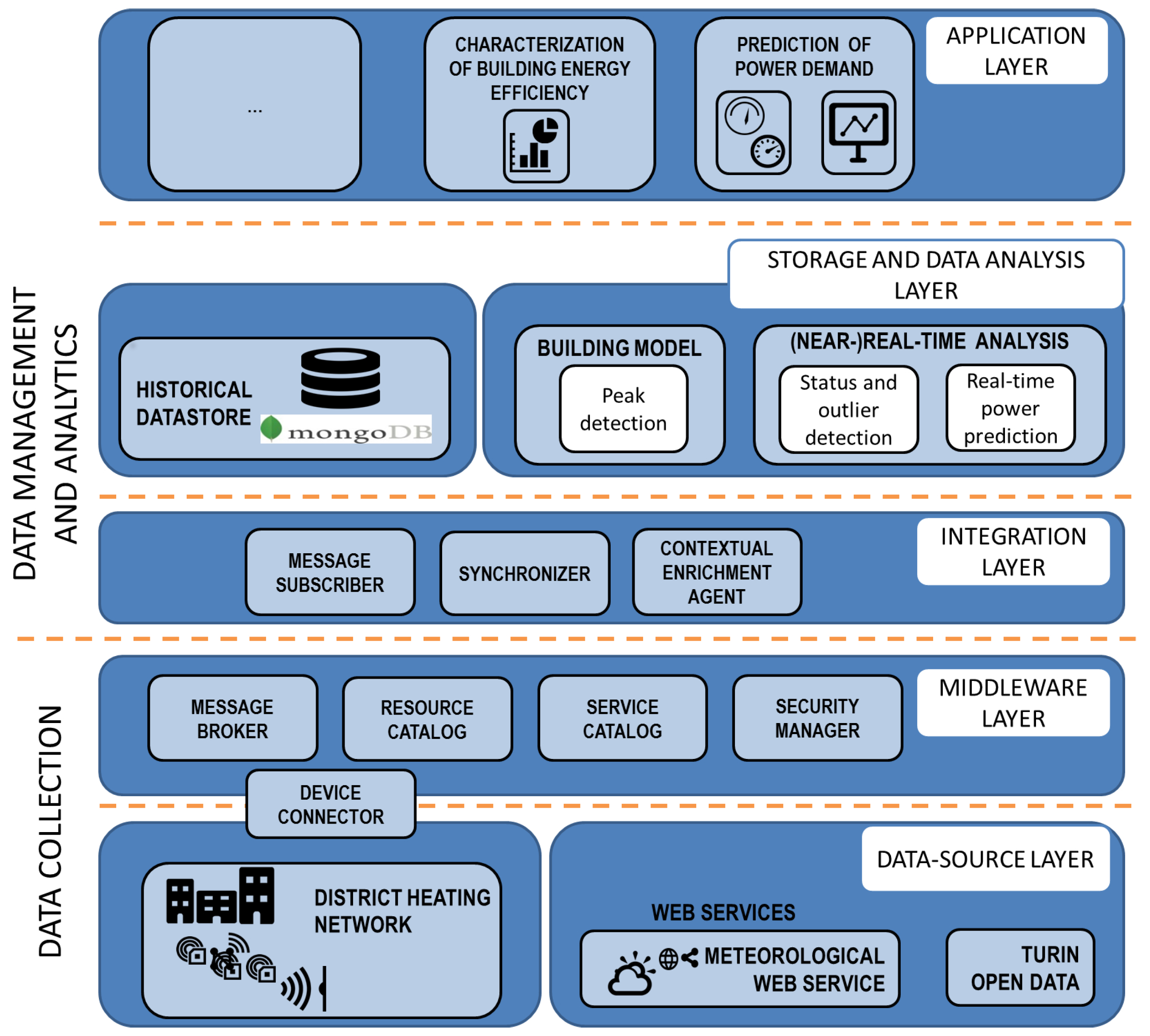
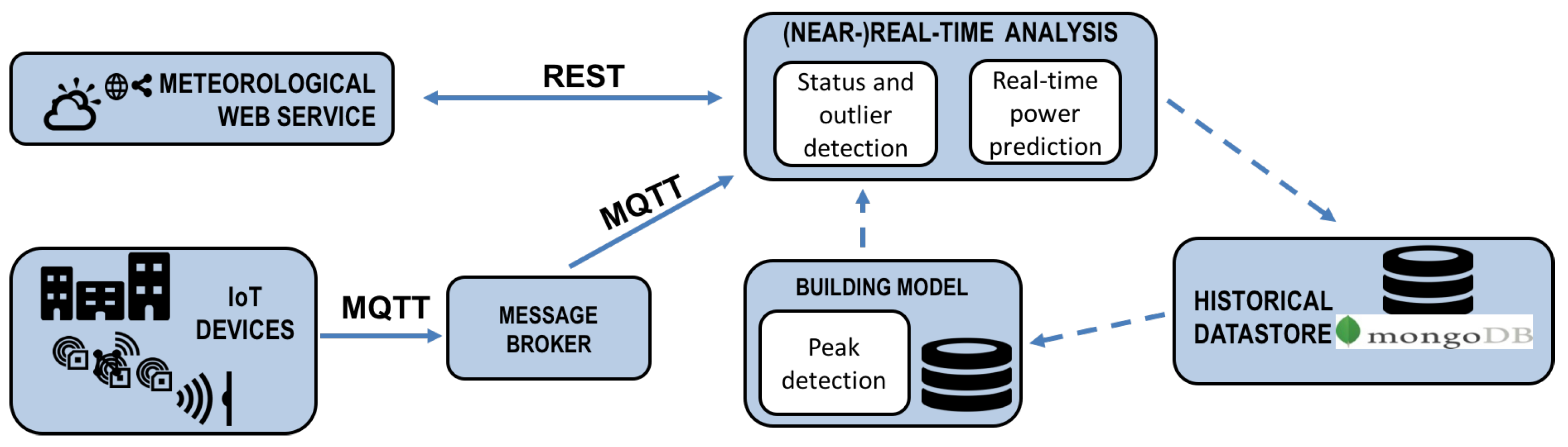
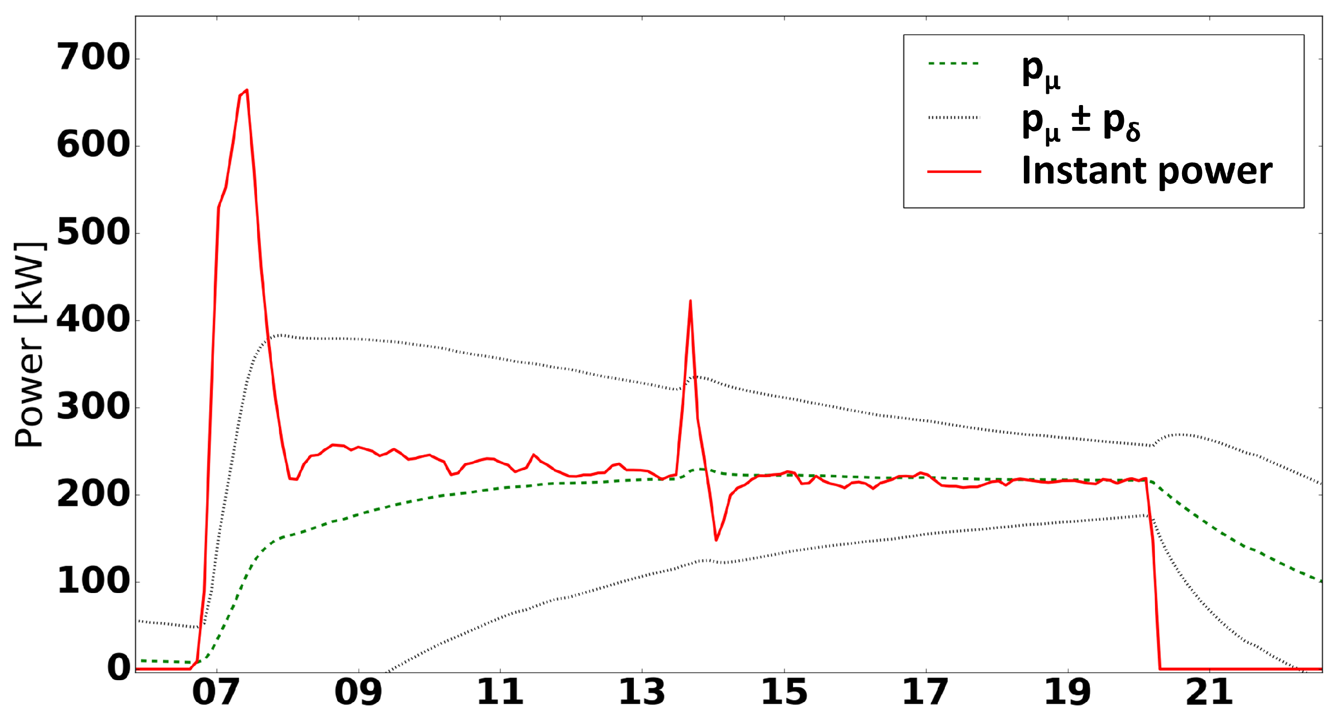
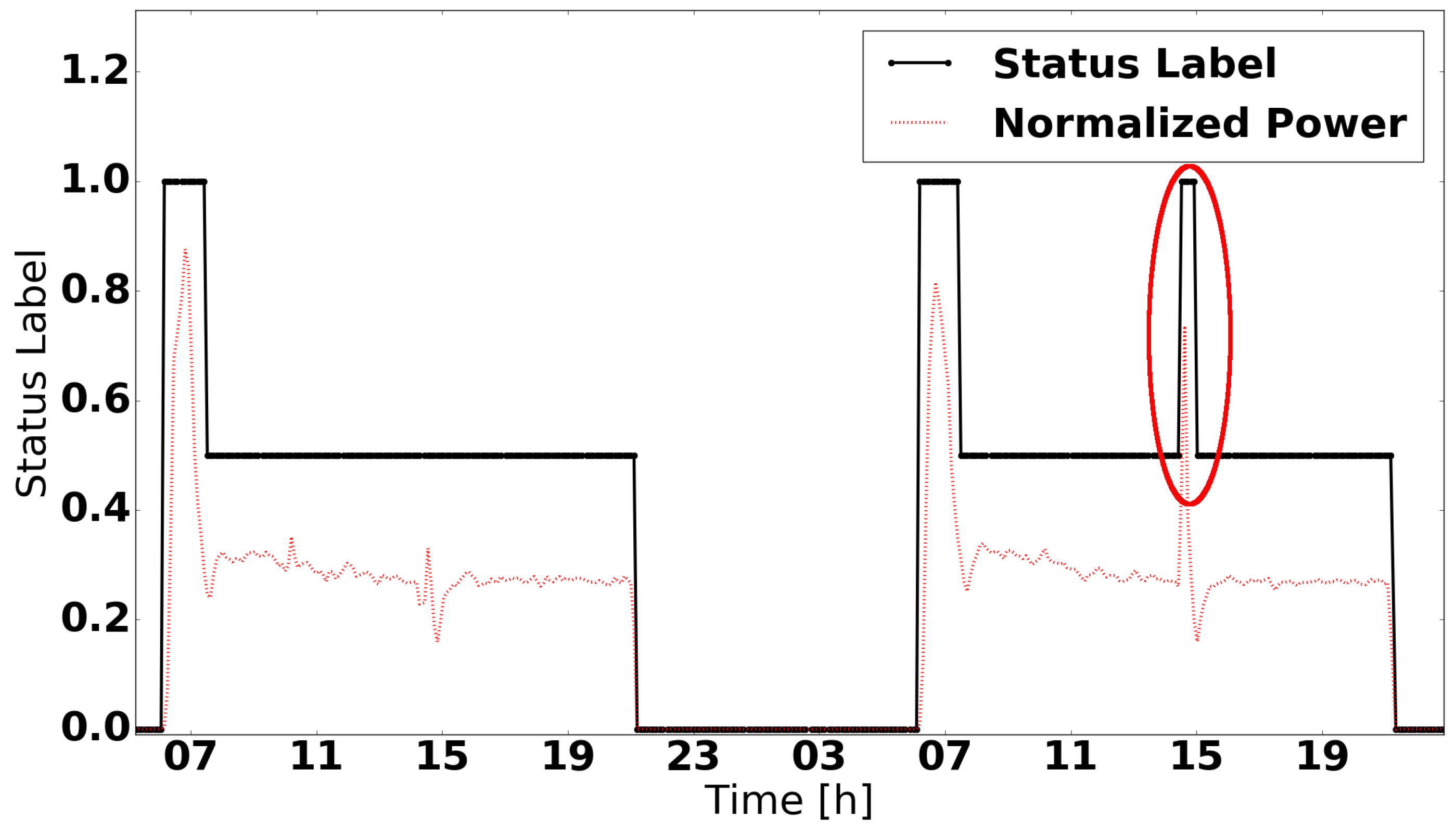
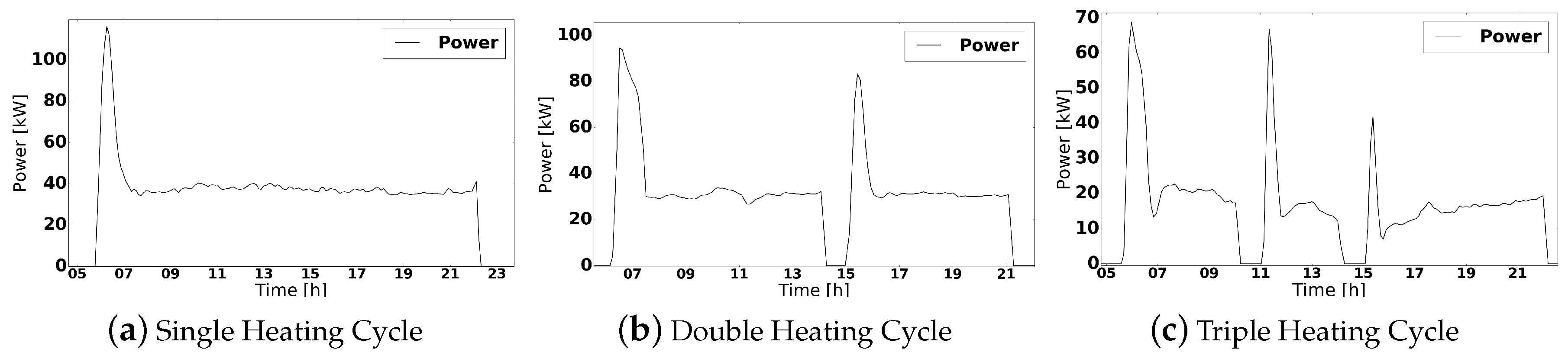
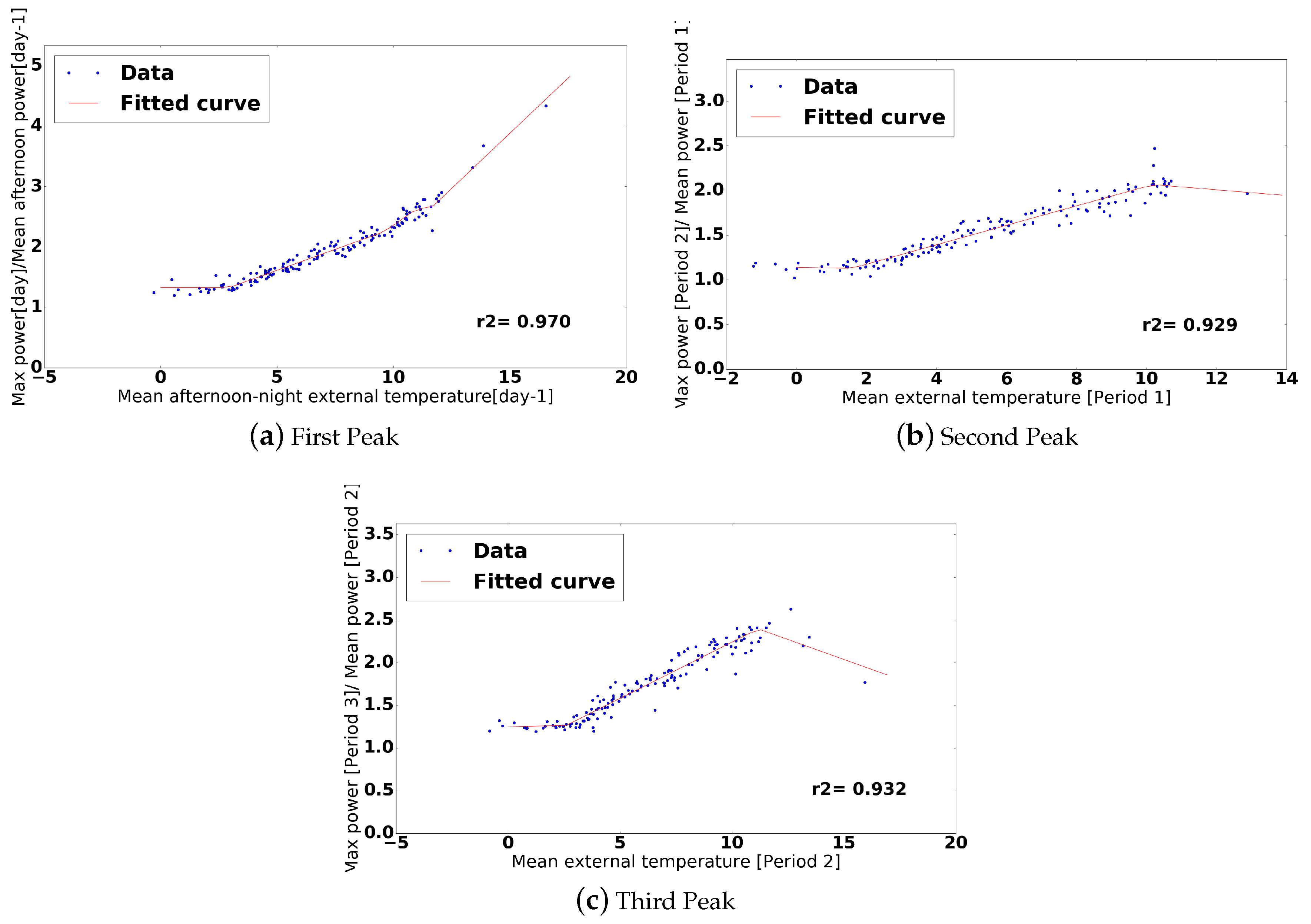
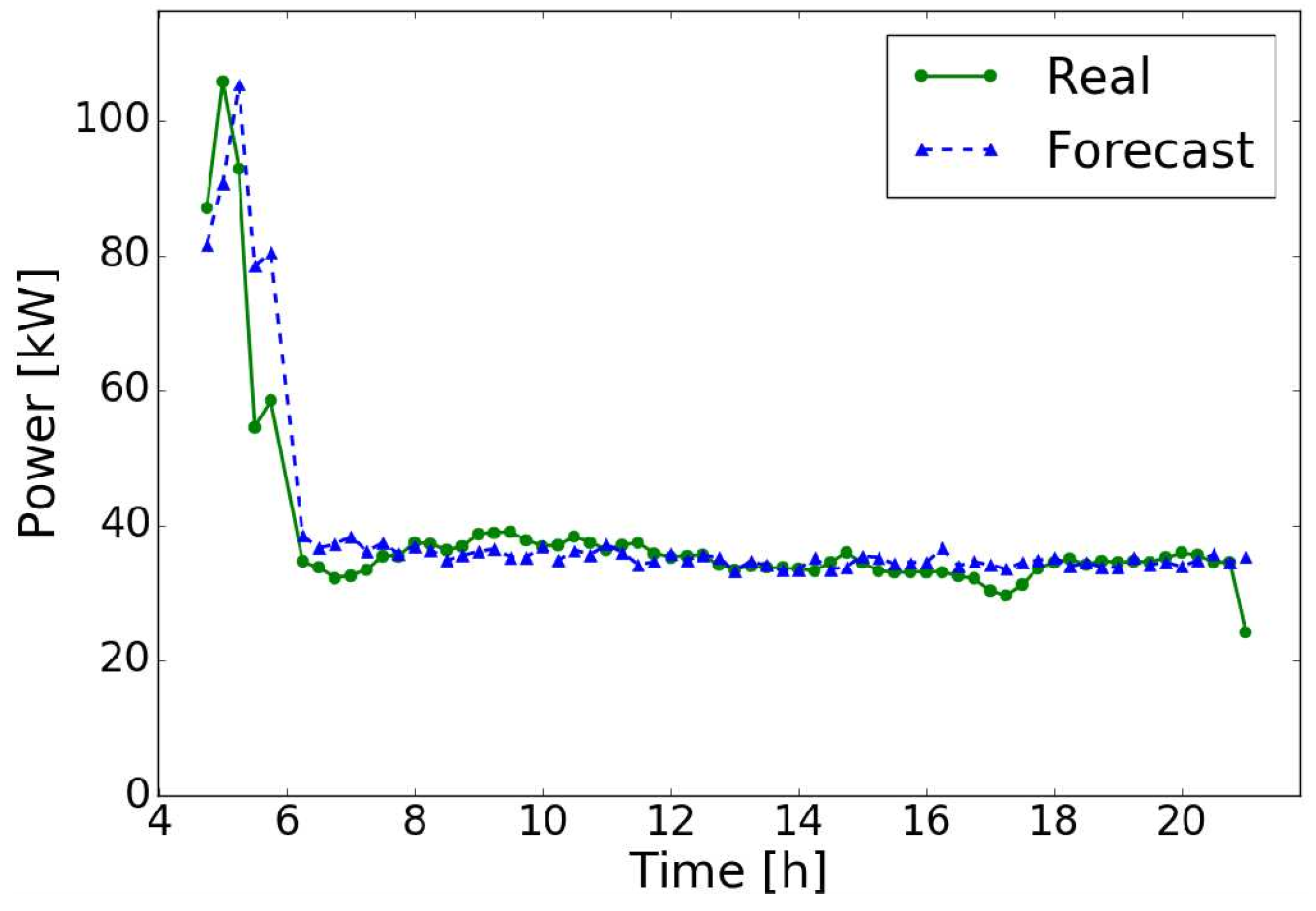
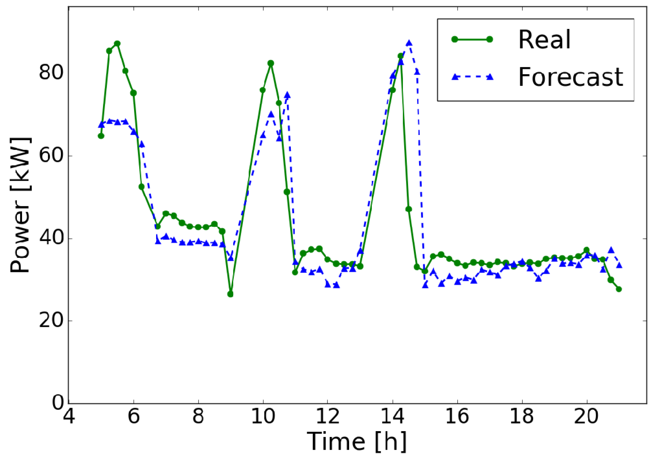
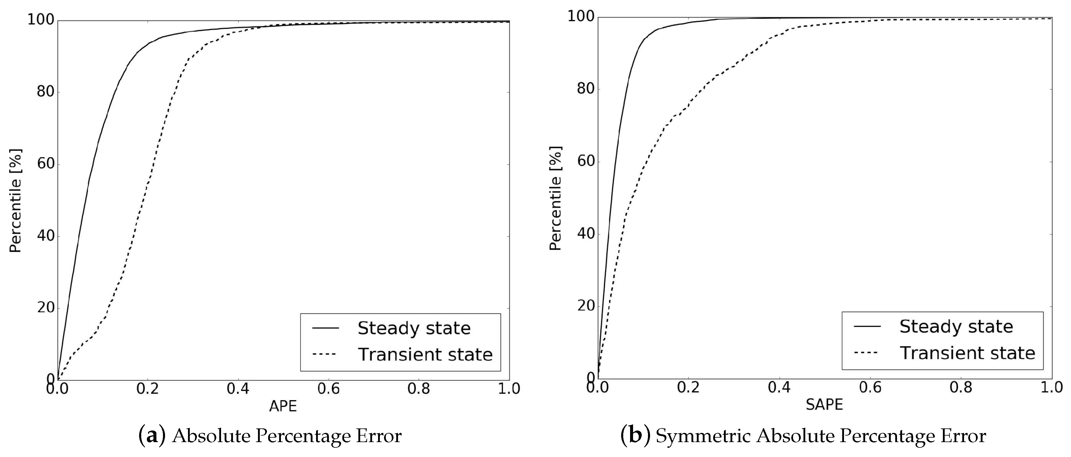
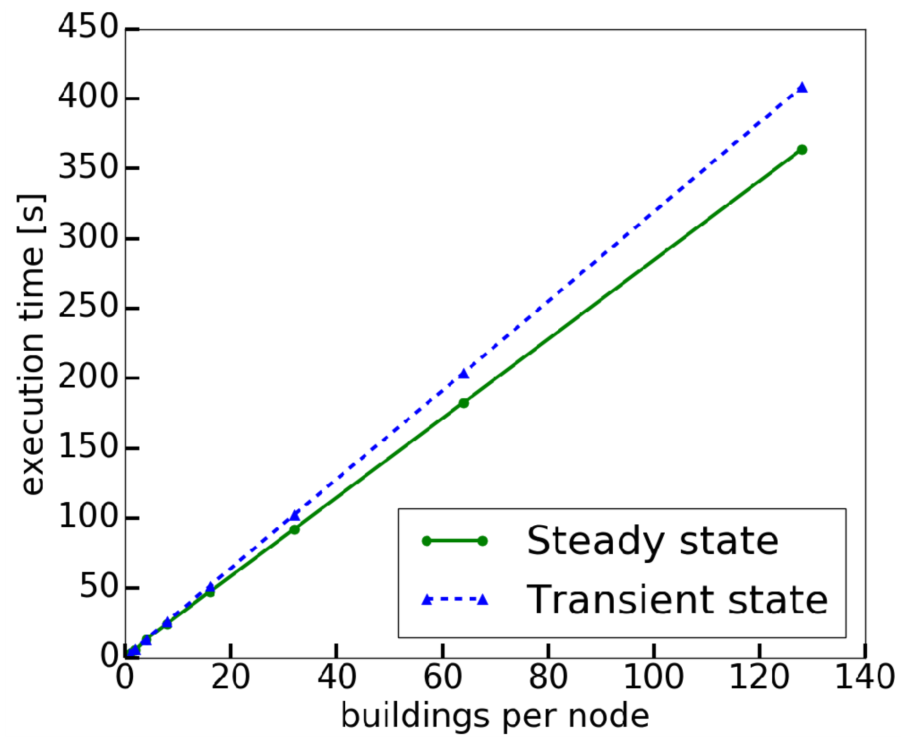
