Design of Robust Fuzzy Logic Controller Based on the Levenberg Marquardt Algorithm and Fault Ride Trough Strategies for a Grid-Connected PV System

Abstract

This paper emphasizes the design and investigation of a new optimization scheme for a grid-connected photovoltaic system (PVS) under unbalance faults. The proposed scheme includes fuzzy logic controller (FLC) based on the Levenberg–Marquardt (LM) optimization technique in coordination with bridge-type-fault-current limiter (BFCL) as the fault ride through (FRT) Strategy. The LM optimization-based control is an iterative process with a fast and robust response and is always convergent. The BFCL reduces the fault currents to rated values without compromising at ripples. A keen and critical comparison of the designed strategy is carried out with a conventionally tuned proportional-integral (PI) controller in coordination with the crowbar FRT strategy. A 100kW MATLAB/Simulink model of a photovoltaic system is used for simulation and analysis of unbalance faults at the point of common-coupling (PCC) and at 5 km away from PCC. It is found that grid-connected PVS is highly influenced by the fault type and less effected by the distribution line length. The simulation results authenticated smooth, stable, ripples with free, robust, and fault-tolerant behavior of the proposed scheme.

1. Introduction

The abrupt advancement in the concept of renewable energy resources (RERs) is due to its technical, economical, reliable, and environmental benefits, which gives way to low scale energy-sources and electrical potential storage devices for low and medium voltages [1]. The RERs offer sustainability in all angles of the energy development sector [2]. Currently, the photovoltaic system (PVS) is contributing a main role to meet global electric power demand among various RERs [3,4,5]. PVS is the most developed RER due to its good looking and flexible nature from residential to commercial loads [6].

The world is compelled to adopt RERs like PVS due to the reduction in greenhouse gas emissions and depletion of fossil fuels for conventional electric power generation [7,8,9]. To achieve the ripple-free and stable output from PVS to be injected toward utility grid, power electronics-based devices like DC to DC boost-converter and maximum-power point-tracker (MPPT) based controls are used. Mostly voltage source inverters (VSI) are employed in inverters because of its simplicity and stability and have both voltage control and current control loops.

According to the last decade statistics, the PVS becomes more sophisticated and its price is declining. The growth of PV plant connections to the grid is increasing rapidly. Therefore, the isolation of PVS from the grid for a long duration is unsuitable for the stability, reliability, and operation of the power system, which can be dangerously affected [10,11]. Thus, for the PV power insertion to the grid, many countries have changed their grid code requirements [12,13,14,15]. The application of these grid code requirements makes sure PVS has the capability to reconnect in a minimum time span after a voltage dip and retaining the grid rated-voltage [16,17]. A German energy company known by E. ON (Energy On) and CEI (Comitato Electtrotecnico Italiano), which is known as a low-voltage-ride-through (LVRT) capacity [12], presents this capability.

The grid stability is achieved by reactive current insertion to reinforce grid voltages during faulty conditions [18,19]. For voltage support, RERs must have to inject reactive current, which amounts to 2% of nominal current for each 1% dip of inverter voltage occurs. Voltage support must be within 20 ms after any abnormality detection [20,21]. The operation of the inverter and PV module can be severely affected by an asymmetrical voltage sag due to high spikes and ripples in the current. Until now, different fault-ride through (FRT) schemes have been introduced to confine LVRT capability under E. ON requirements to overcome this problem [22,23,24,25,26,27,28,29,30]. Most of the previously proposed strategies have minimized the fault current. However, it is compromised at high ripples and vice versa [22,23]. Active and reactive power control is carried out, which results in non-sinusoidal current response during an unbalance fault [24,25]. According to Reference [26], a positive and negative sequence balance control is proposed, but the issue of oscillations in harmonics with both active and reactive components injection is not eliminated. Most of the above-mentioned articles have emphasized the proportional-integral (PI) and proportional-resonant (PR) controllers for inverter control and a conventional crowbar as the FRT strategy to achieve LVRT capability for PVS.

Since the PI controller has enormous use in industries due to its simplicity, it has some restrictions due to its nonlinear response to the dynamic system i.e., fault conditions and sensitivity toward parametric uncertainties. Until now, the conventional crowbar is used as the FRT strategy to limit the effect of fault current at an inverter even though it violates the requirements of grid connection and utility to retain normal operation [29].

To handle the above-mentioned problems, we are presenting a novel FLC based on the Levenberg–Marquardt (LM) technique for the inverter control in combination with bridge-type-fault-current limiter (BFCL) as the FRT strategy to optimize fault parameters of grid-connected PVS under unbalance abnormal conditions. LM-based optimization uses the hybrid algorithm, which has characteristics of high speed of Gauss-Newton method and fast convergence of the Steepest Descent method. This is why it can respond efficiently during dynamic conditions, which is the deficiency of the PI controller. Moreover, the proposed BFCL includes special arrangements of the bridge path, which significantly reduces the di/dt stress on the controlled switch due to a change of the half cycle and fault transients. A detailed model of the 100-kW PV array connected to the utility grid is taken from SimPower examples of MATLAB/Simulink for simulations to justify our proposed scheme.

1)

A 100kW MATLAB/Simulink model of photovoltaic system is used for simulation at both the grid side and the PV side variables and dc-link voltage are kept within optimum limits during asymmetrical faults at PCC. Moreover, the proposed strategy is employed at 5 km from PCC to investigate the variations due to the distribution line impedance during the fault.

2)

A novel bridge-type-fault-current limiter (BFCL) strategy is employed to strengthen the LVRT capability of three-phase grid connected PVS comfortably.

3)

A comprehensive and keen comparison of conventional-crowbar circuitry with the BFCL strategy is performed to authenticate the optimized and smooth response of the system variable with the BFCL strategy.

4)

LM is designed and compared precisely with a previously adopted conventional PI controller. Due to the robust nature, the LM optimization-based controller is fast and always convergent.

5)

Unbalance faults are applied for 0.15 s to verify the fault-tolerant capability of the proposed LM in coordination with BFCL when compared to a conventional PI and crowbar strategy.

6)

Performance evaluation analysis is performed to verify stability of the proposed controller and strategy i.e., Integral-Absolute-Error (IAE), Integral-Square-Error (ISE), and Integral of Time-Weighted-Absolute-Error (ITAE).

7)

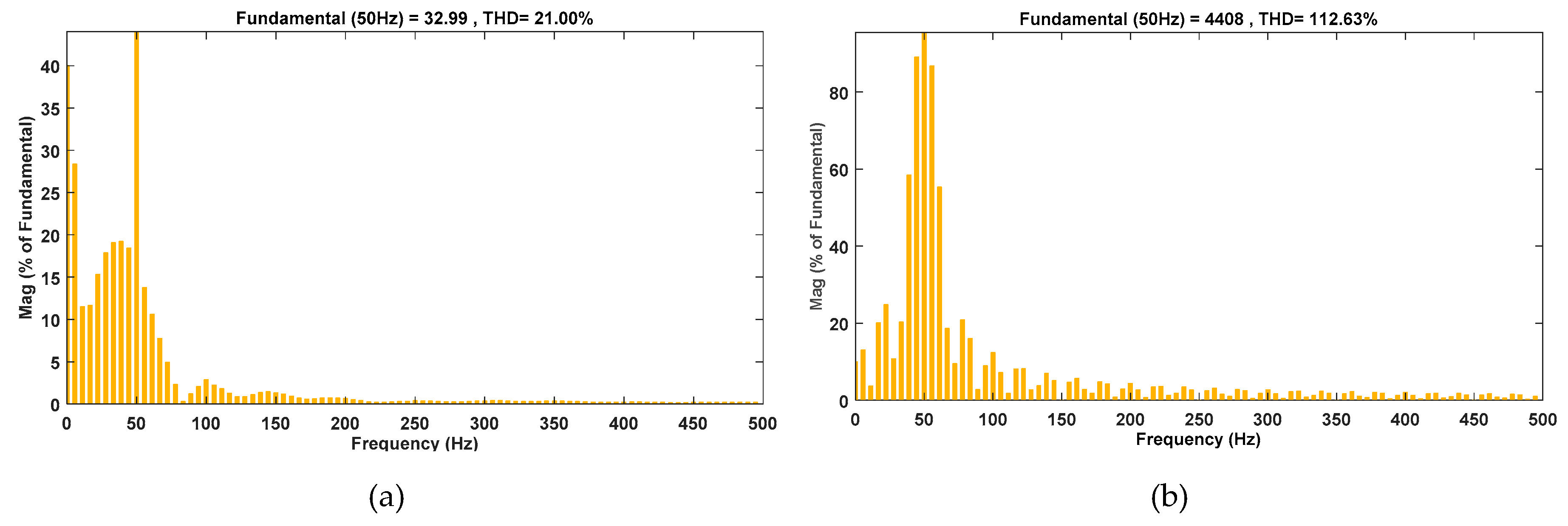
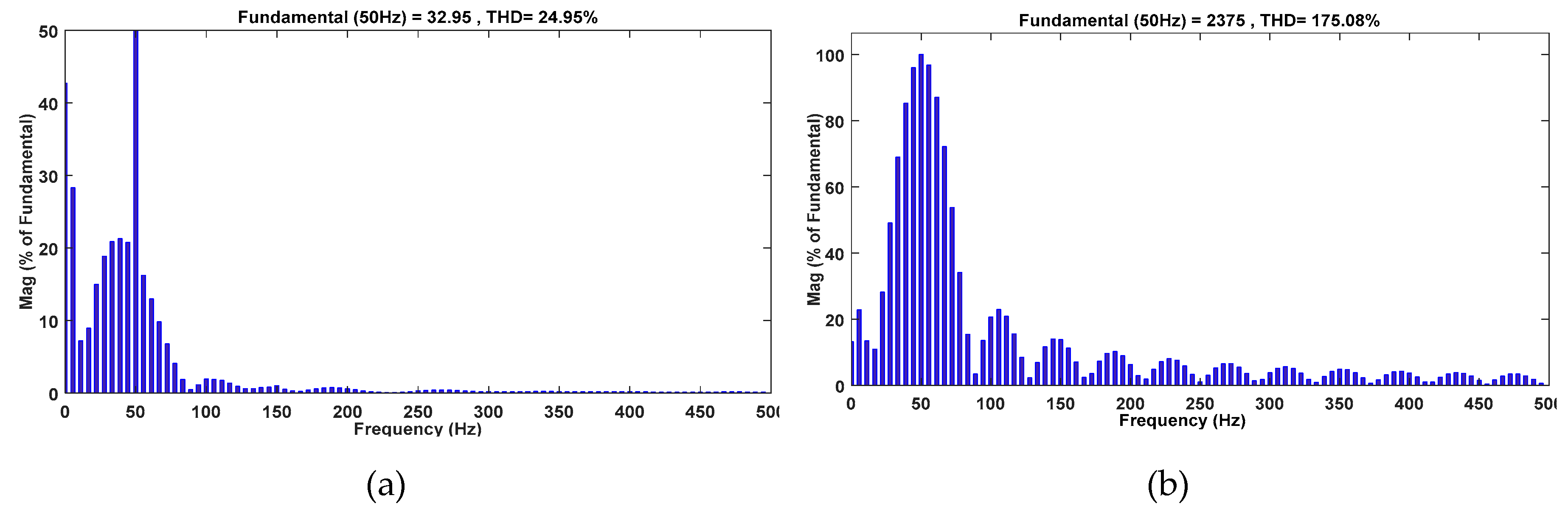
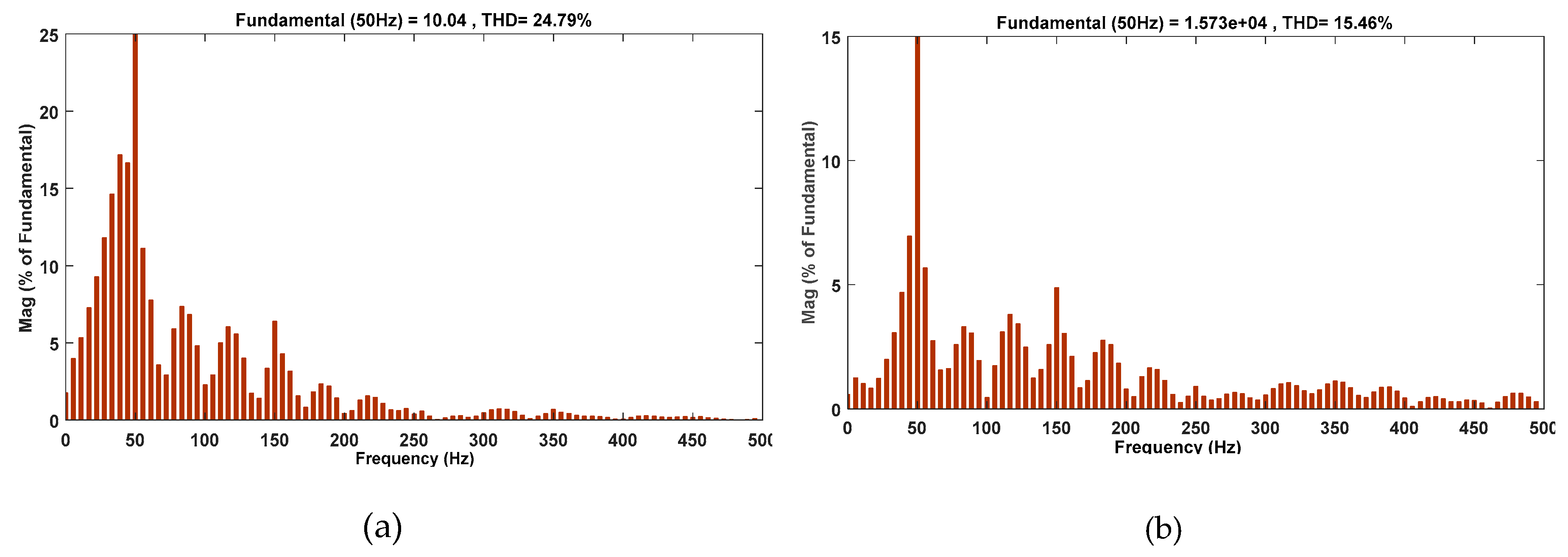
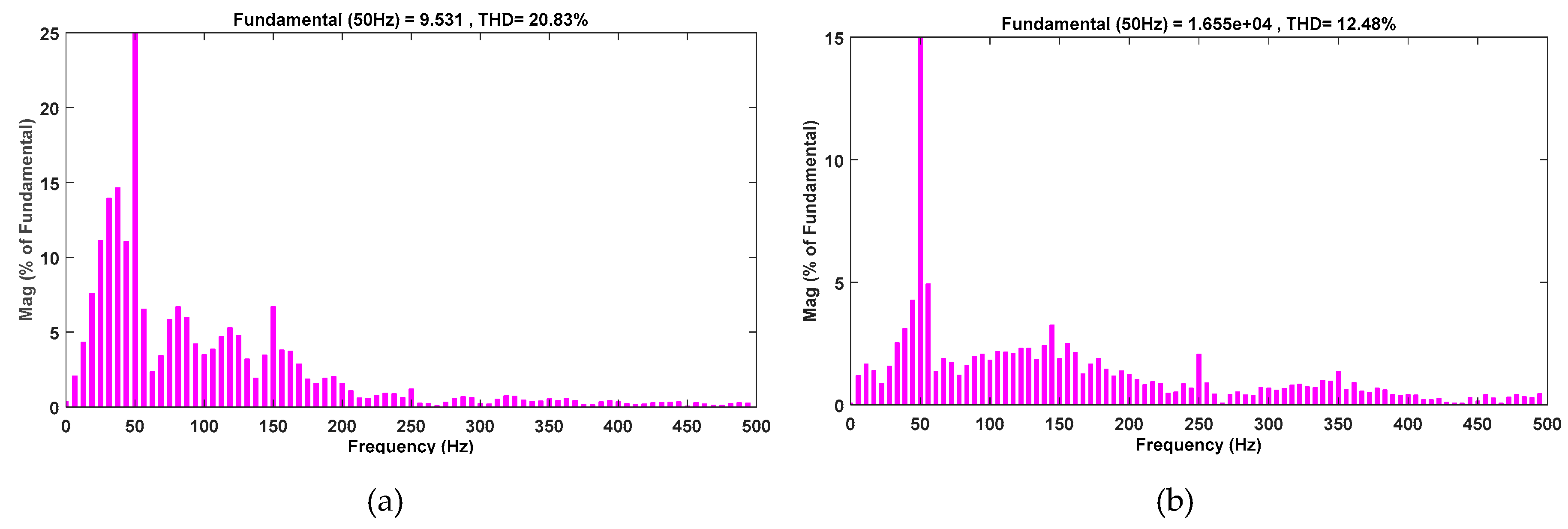
Total harmonic distortion (THD) is calculated using fast fourier transform (FFT) analysis for grid current and voltage to validate the robustness of the proposed approach.

The article is organized under sections where Section 2 presents the modeling of the PV system with the help of subsections like mathematical modeling of the PV cell, mathematical modeling of the DC-to-DC boost-converter, and mathematical modeling of the voltage-source inverter, the proposed model, and the design of the controller along with the FRT strategy. Results and discussion are covered in Section 3 and paper concludes in Section 4.

2. Mathematical Modeling

An overview of the mathematical modeling of some important blocks of the proposed model are illustrated below.

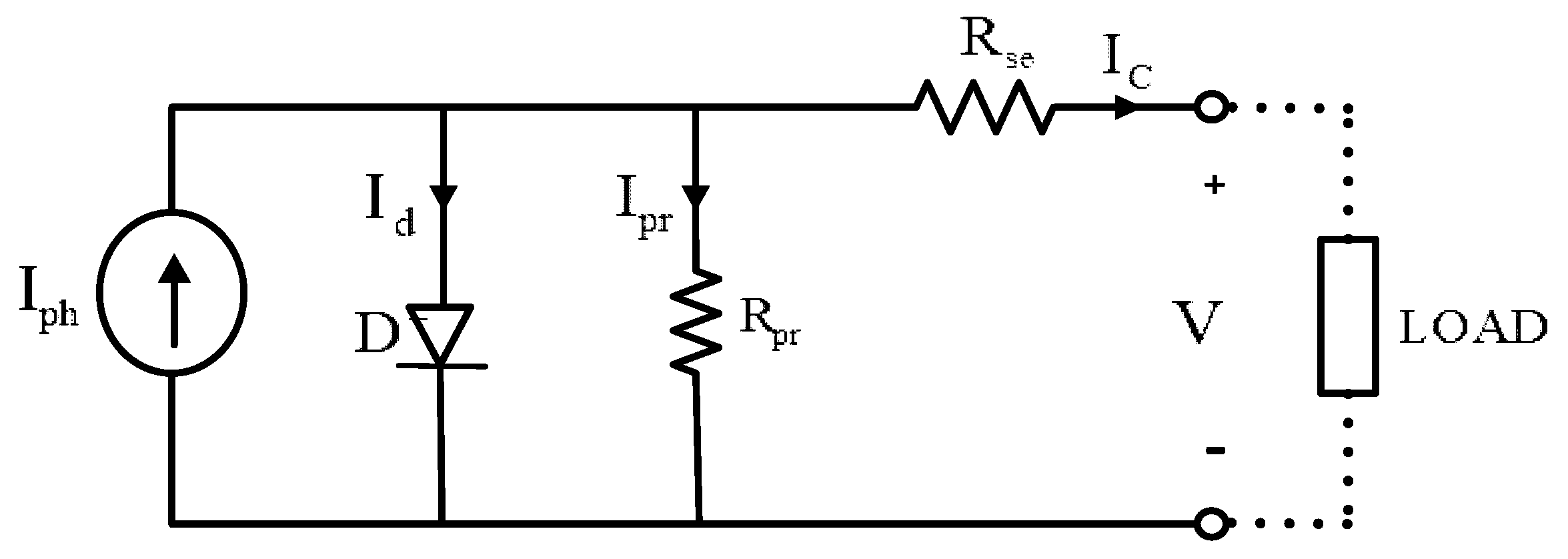
2.1. Mathematical Modeling of the PV Cell

A PV cell is a semiconducting p-n layer. When exposed to the light, it becomes forward biased and conducts current. The generated current from the solar cell depends linearly on sun irradiance. Practically no solar cell exists that is ideal. Therefore, the circuit model is represented by a high parallel resistance ($R_{pr}$) and a small series resistance ($R_{se}$). The equivalent model is presented by Figure 1 below.

Therefore, by Kirchhoff’s current law (KCL), we acquired the equation below.

$${\mathrm{I}}_{\mathrm{c}}={\mathrm{I}}_{\mathrm{ph}}-\left({\mathrm{I}}_{\mathrm{d}}+{\mathrm{I}}_{\mathrm{pr}}\right)$$

(1)

$${\mathrm{I}}_{\mathrm{C}}={\mathrm{I}}_{\mathrm{ph}}-\left[{\mathrm{I}}_{\mathrm{sat}}.\left\{\exp \left(\frac{\mathrm{V}+{\mathrm{I}}_{\mathrm{c}}.{\mathrm{R}}_{\mathrm{se}}}{{\mathrm{V}}_{\mathrm{T}}}\right)-1\right\}+\left\{\frac{\mathrm{V}+{\mathrm{I}}_{\mathrm{c}}.{\mathrm{R}}_{\mathrm{se}}}{{\mathrm{R}}_{\mathrm{pr}}}\right\}\right]$$

(2)

Here,

• ${\mathrm{I}}_{\mathrm{c}}$: Output current (A) of PV cell
• ${\mathrm{I}}_{\mathrm{sat}}$: Reverse saturation current of diode = 5.261 × 10⁻⁹ A
• ${\mathrm{I}}_{\mathrm{ph}}$: Insulation current = 5.958 A
• ${\mathrm{R}}_{\mathrm{se}}:$ 0.0831 ohms
• ${\mathrm{R}}_{\mathrm{pr}}:$ 8192 ohms
• ${\mathrm{V}}_{\mathrm{T}}$: Thermal voltage, calculated by Equation (3) below.

$${\mathrm{V}}_{\mathrm{T}}=\frac{\mathrm{KT}}{\mathrm{q}.\mathrm{Qd}.\mathrm{Npr}.\mathrm{Nse}}$$

(3)

Here, $\mathrm{K}$ is the Boltzmann constant = 1.3806 × 10⁻²³ (j/k)

• $\mathrm{T}$: Absolute Temperature = 25 °C
• ${\mathrm{Q}}_{\mathrm{d}}:$ Quality factor of diode = 1.25
• $\mathrm{q}:$ Charge of electron = 1.602 × 10⁻¹⁹ C
• ${\mathrm{N}}_{\mathrm{pr}}:$ Number of parallel strings = 66
• ${\mathrm{N}}_{\mathrm{se}}:$ Number of series-connected modules/string = 5

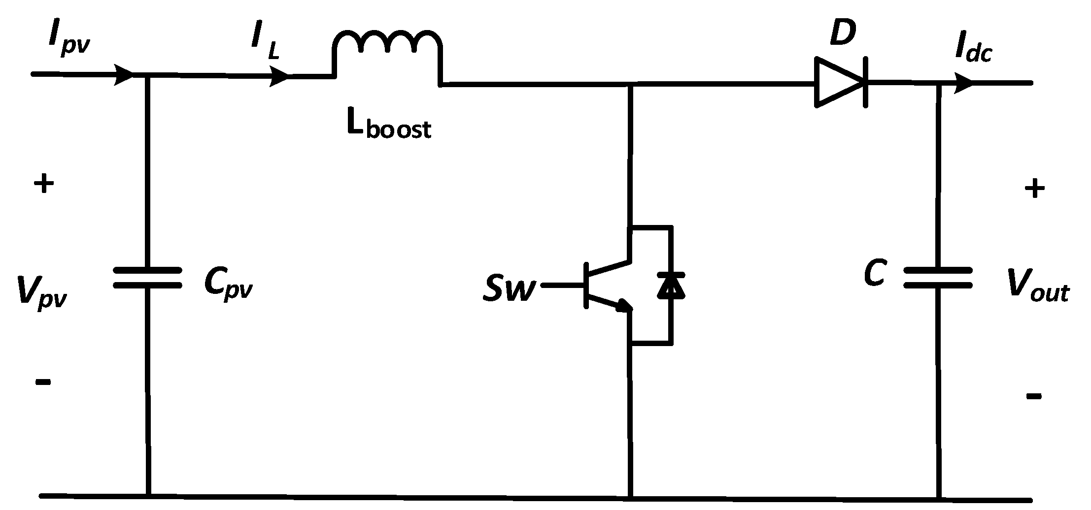
2.2. Mathematical Modeling of the DC-to-DC Boost-Converter

All over the world, different techniques i.e., single-stage and two-stage have been followed to obtain maximum-power-point-tracking (MPPT) for grid-connected PV systems. Although, the proposed model uses two-stage methodology since it can efficiently boost PV voltage to an optimal value for the inverter. The system also becomes economical. It is performed by the power electronic switch, which is controlled by the duty-cycle of the converter. The DC to DC boost-converter model with essential components i.e., input dc voltage, which is the output of the PV module (V_PV), boost-inductor (L_boost), switch (SW), a diode (D), and a filtering capacitor (C) as depicted by Figure 2. To minimize harmonics up to a high extent in frequency, a capacitor (C_pv) is carried out between the PV module and DC-DC circuit, which is given by equation (4) [31].

$${\mathrm{C}}_{\mathrm{PV}}=\frac{{\mathrm{DV}}_{\mathrm{PV}}}{4\Delta {\mathrm{V}}_{\mathrm{PV}}{\mathrm{f}}_{\mathrm{sw}}{}^2{\mathrm{L}}_{\mathrm{boost}}}$$

(4)

• D: Duty Cycle of Boost-Converter.
• V_PV: Input voltage for boost-converter = 273 V.
• ${\mathrm{f}}_{\mathrm{sw}}:$ Switching frequency of boost converter = 5 KHz.
• ${\mathrm{L}}_{\mathrm{boost}}:$ Boost inductor = 5 mH.

The boost inductor value can be calculated by using the equation below [32].

$${\mathrm{L}}_{\mathrm{boost}}=\frac{{\mathrm{V}}_{\mathrm{in}}.\left({\mathrm{V}}_{\mathrm{out}}-{\mathrm{V}}_{\mathrm{in}}\right)}{\Delta {\mathrm{I}}_{\mathrm{L}}.{\mathrm{f}}_{\mathrm{sw}}.{\mathrm{V}}_{\mathrm{out}}}$$

(5)

Here,

$$\Delta {\mathrm{I}}_{\mathrm{L}}={\mathrm{I}}_{\mathrm{out}}\frac{{\mathrm{V}}_{\mathrm{out}}}{{\mathrm{V}}_{\mathrm{in}}}$$

(6)

• ${\mathrm{V}}_{\mathrm{out}}$: Boost converter output voltage = 500 V.

The duty cycle, obtained from the equation of voltage balance, is given below as:

$$\mathrm{D}=1-\frac{{\mathrm{V}}_{\mathrm{PV}}}{{\mathrm{V}}_{\mathrm{dc}\mathrm{Link}}}$$

(7)

The duty cycle (D) of the boost-converter is controlled to track maximum-power-point for PVS.

2.3. Mathematical Modeling of Inverter

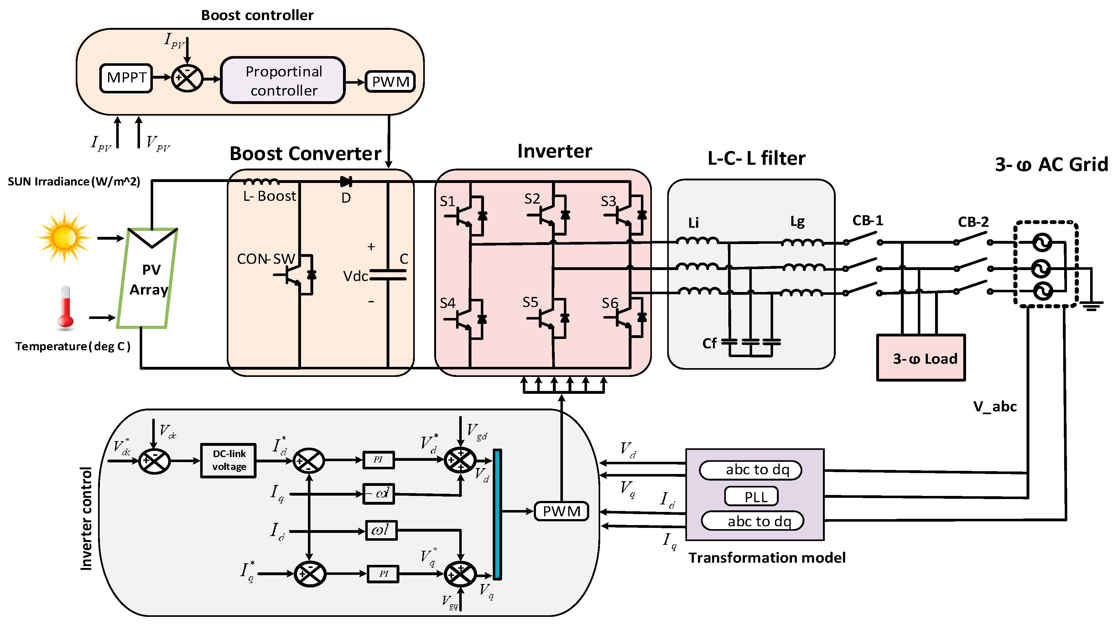
The most important area in a grid-connected PVS is the inverter control rather than the maximum power point achievement. The inverter control environment is responsible for pulse width modulation (PWM) generation, grid synchronization, and monitoring power flow. Two topologies of inverters are adopted widely to convert the DC source to the AC source, which are the “voltage-source-inverter (VSI)” and the “current-source-inverter (CSI).” Normally, the VSI type three-phase inverters are used for grid-connected PVS since it provides a constant sinusoidal waveform of voltage. The proposed 3-phase VSI is designed by using six IGBTs switches in the MATLAB/Simulink [33]. A synchronous reference frame is used for simplification of the control.

The following matrix equations are calculated to convert voltage and current from a natural to a synchronous (d-q) reference frame.

$$\left[\begin{array}{c}{\mathrm{v}}_{\mathrm{d}}\\ {\mathrm{v}}_{\mathrm{q}}\end{array}\right]=\sqrt{\frac{2}{3}}\left[\begin{array}{ccc}\sin \mathsf{\omega }\mathsf{\tau }& \sin \left(\mathsf{\omega }\mathsf{\tau }-\frac{2\mathsf{\pi }}{3}\right)& \sin \left(\mathsf{\omega }\mathsf{\tau }+\frac{2\mathsf{\pi }}{3}\right)\\ \cos \mathsf{\omega }\mathsf{\tau }& \cos \left(\mathsf{\omega }\mathsf{\tau }-\frac{2\mathsf{\pi }}{3}\right)& \cos \left(\mathsf{\omega }\mathsf{\tau }+\frac{2\mathsf{\pi }}{3}\right)\end{array}\right]$$

(8)

$$\left[\begin{array}{c}{\mathrm{i}}_{\mathrm{d}}\\ {\mathrm{i}}_{\mathrm{q}}\end{array}\right]=\sqrt{\frac{2}{3}}\left[\begin{array}{ccc}\sin \mathsf{\omega }\mathsf{\tau }& \sin \left(\mathsf{\omega }\mathsf{\tau }-\frac{2\mathsf{\pi }}{3}\right)& \sin \left(\mathsf{\omega }\mathsf{\tau }+\frac{2\mathsf{\pi }}{3}\right)\\ \cos \mathsf{\omega }\mathsf{\tau }& \cos \left(\mathsf{\omega }\mathsf{\tau }-\frac{2\mathsf{\pi }}{3}\right)& \cos \left(\mathsf{\omega }\mathsf{\tau }+\frac{2\mathsf{\pi }}{3}\right)\end{array}\right]$$

(9)

The required voltage waveforms achieved through the current-controller are further used to obtain the triggering pulse for the three-phase inverter using a pure sine wave. The obtained voltage-wave forms are further convolved with a triangular carrier wave of frequency 30-kHz and, by using reverse matric calculations, the parameters in the synchronous frame are again converted to the natural frame.

2.4. Proposed Model

A built-in detailed model of the 100-kW PV array connected to the utility grid is taken from SimPower examples of MATLAB/Simulink R2014 for simulations to justify our proposed strategy. “Pierre Giroux” designed this detailed model in the Hydro-Quebec Research Institute (IREQ) by “Pierre Giroux.” The model parameters are extracted from the National Renewable Energy Laboratory (NREL) system advisor model (SAM) for reference (https://sam.nrel.gov/). All the parameters of the system are kept unchanged. Only the proposed FRT strategy and controller are applied for their performance verification. These system parameters include a 100-kW PV array, which transfers power through a 20 KV distribution transformer to a 110 KV power grid. The DC-to-DC boost converter and a 3-phase 3-level inverter (VSI) are employed for the PV array, as depicted in Figure 3. The PV power generator is comprised of 66-parallel connected strings. Each string consists of 5-series connected modules (330 SunPower SPR-305-WHT) [34]. The PV array takes sun irradiance and temperature in watts per meter-square (W/m²) and Centi-grades(C), respectively.

The DC-to-DC boost converter with 5 kHz of switching frequency is employed to boost up the PV array output voltage i.e., 273V to 500V, which is a DC-link voltage. Moreover, the MPPT is achieved in the DC-to-DC converter by adopting the incremental conductance algorithm [35]. By using this type of MPPT algorithm, the duty cycle is automatically changing to extract a maximum power point.

A three-phase three-level VSI inverts the DC-link voltage to alternating 260 V with 2 kHz of switching frequency. The control structure of VSI includes two control loops i.e., internal control loop and external control loop to interact DC-link voltage with the grid. The internal control loop regulates active (Id) and reactive (Iq) parts of current. However, for the sake of the unity power factor, Iq_ref is kept to zero. Although, the external loop regulates the DC-link voltage for two split capacitors. The synchronous reference frame current controller output is transformed to a modulating signal U_(abc_ref), which is used for pulse generation.

For controlling the inverter parameter in the d-q frame, the proposed “LM optimization based FLC “is implemented. However, the grid-connected PVS variables during fault current, voltage, and power are optimized by introducing a new FRT strategy i.e., BFCL. The conventionally used PI controller and a crowbar as FRT are also simulated at PCC and at 5-km distance from PCC to verify the robustness of the proposed scheme. Additionally, the overall model parameters are given in

Table A1. Model rated parameters.

Parameters	Values
PV power	100.6 kW
PV module voltage	273 V (L-L, rms)
No. of Phases	3
Full-Load current of PV	364 A
System operating frequency	50 Hz
Boost-converter frequency	5 kHz
Vdc	500 V
Grid voltage	20 KV
Choke impedance (R, L)	2×10−3 ohm, 2.5×10−6 H
Sun irradiance for PV	1000 (W/m2)
Temperature	25 °C
Algorithm used for MPPT	Incremental conductance
Full -load current of grid	2.94 A
Switching frequency of inverter	2 kHz

of Appendix A.

2.5. Design of the Controller and FRT Strategy

Due to the various topologies of the grid-connected inverter, different types of control and FRT schemes have been introduced for the protection of PVS. The control schemes are responsible for keeping the dc-link voltage at a desired reference. However, FRT strategies are designed to optimize fault variables under any fault condition of grid-connected PVS such as restricted fault currents, grid synchronism, constant power, and phase sequence.

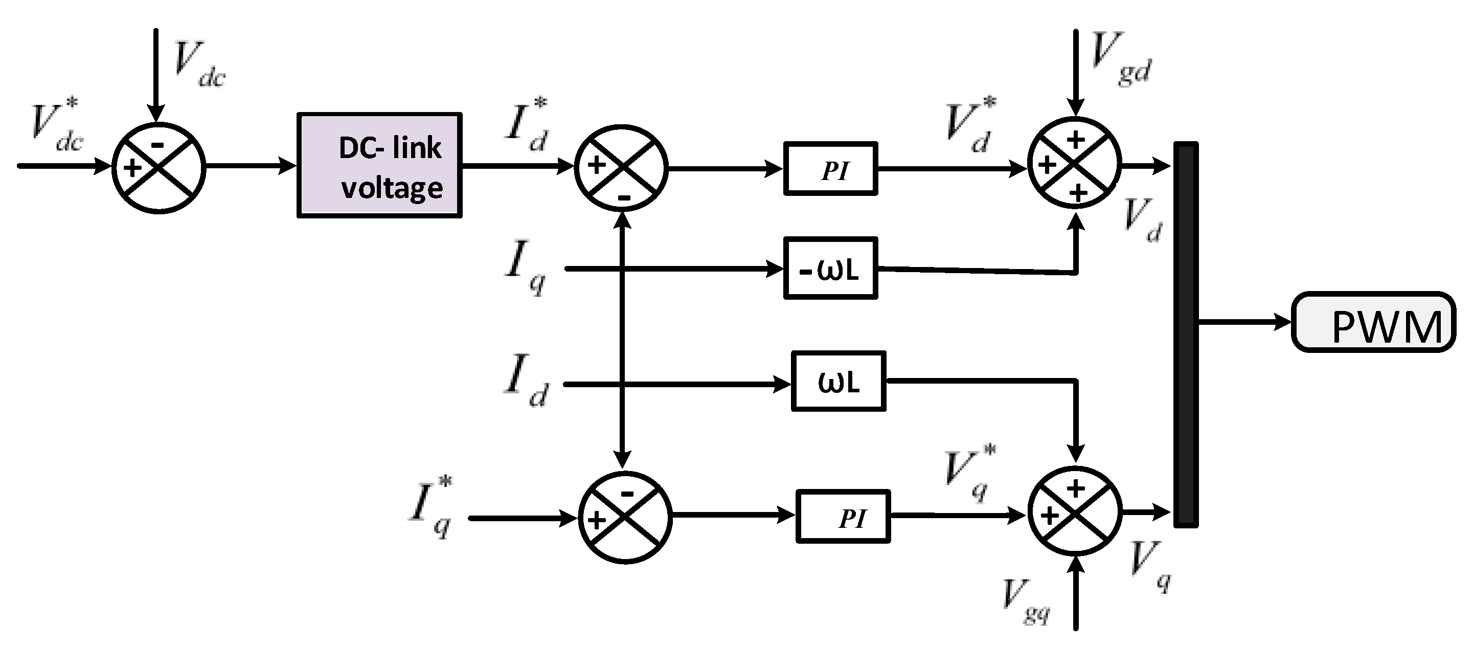
2.5.1. Controller Design

To demonstrate the proposed control for balancing the power of voltage-source-inverter (VSI), a short description is given below.

Proportional-Integral (PI) Controller

Figure 4 below depicts the control structure of the inverter based on a PI controller, which describes the comparison and measurement of DC-link voltage using the dq-reference frame. The dq-frame is adopted by the PI controller instead of the natural frame due to its simplicity and efficient behavior for the dc variable operation. By adopting the dq frame, the desired variables to control are converted to the dc frame so that their control become simple [36]. It is a dual loop control, which generates compensated current reference by the outer loop i.e., voltage loop. The voltage loop gives output in the form of current as the Id reference and the Iq reference. However, the Iq reference is kept at zero for the sake of the unity power factor. The inner control loop i.e., current loop output voltage components in the dq-frame are again converted to a natural frame with three modulating signals to generate PWM. Moreover, the controller’s parameter values are given in

Table A2. Control scheme constants.

Control Schemes	Parameters	Vdc	Id	Iq
PI	${\mathrm{k}}_{\mathrm{p}}$	7	0.3	0.3
	${\mathrm{k}}_{\mathrm{i}}$	800	20	20
FLC base on LM	${\mathrm{c}}_1$	0.4	0.2	0.2
	${\mathrm{c}}_2$	1.2	0.6	0.6
	${\mathsf{\sigma }}_1$	0.4	0.2	0.2
	${\mathsf{\sigma }}_2$	0.8	0.4	0.4
	${\mathrm{b}}_1$	0.4	0.2	0.2
	${\mathrm{b}}_2$	1.2	0.6	0.6
	λ	1.9	1.9	1.9
	$\mathsf{\mu }$	0.62	0.62	0.62

of appendix.

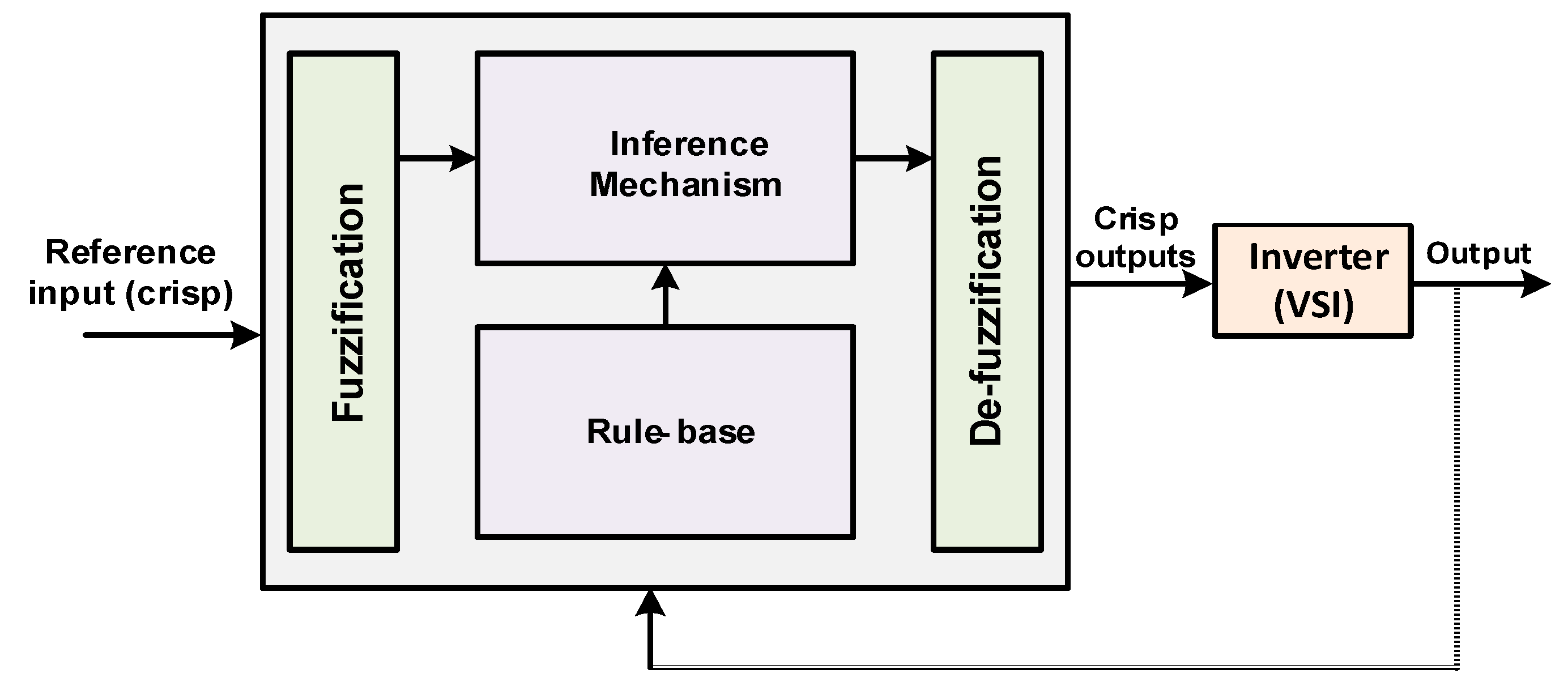
Fuzzy Logic (FLC) Controller Based on Levenberg–Marquardt (LM) Optimization

In this section, the design and investigation of the proposed FLC based on LM optimization is discussed. Until now, different types of control schemes have been introduced to control the grid connected inverter, with their own favorable properties. LM rule-based FLC is more efficient for inadequately understandable, complex kinetics and non-linear systems. This proposed control is directly adoptable, which does not need any mathematical model. The unpredictable nature of the non-linear system can be managed by changing the center of the singleton Membership Function [37].

Due to slow and small step sizes, the training process of the Steepest-Descent (SD) algorithm always results in convergence [38]. However, the Gauss-Newton (GN) algorithm results in a minimum error and has a fast response than SD, but with a high probability of divergence. Whenever the inverse of the Jacobian matrix approaches infinity, the GN algorithm fails. Therefore, to avail the convergence characteristic of SD and fast response of GN, a hybrid methodology is adopted i.e., LM, which is also stable to the Jacobian matrix [39]. Moreover, problems like “least square non-linear minimization” are sorted out through the LM-based control.

$$\mathrm{f}\left(\mathrm{x}\right)=\frac{1}{2}{\displaystyle \sum }_{\mathrm{j}=1}^{\mathrm{m}}{\mathrm{r}}_{\mathrm{i}}^2\left(\mathrm{x}\right).$$

(10)

In the above Equation (10) vector, $\mathrm{x}={\left[{\mathrm{x}}_1{\mathrm{x}}_2{\mathrm{x}}_3\cdots {\mathrm{x}}_{\mathrm{n}}\right]}^{\mathrm{T}}\in {\mathrm{R}}^{\mathrm{n}\times 1}$. Here, $\mathrm{x}$ is a vector that belongs to ${\mathrm{R}}^{\mathrm{n}\times 1}$ and each ${\mathrm{r}}_{\mathrm{i}}$ is the function from ${\mathrm{R}\mathrm{to}\mathrm{R}}^{\mathrm{n}}$. The ${\mathrm{r}}_{\mathrm{i}}$ is known as the residuals and it is supposed that $\mathrm{m}\ge \mathrm{n}$. LM optimization is learned from the following iterative equation.

$${\mathrm{w}}_{\mathrm{k}+1}={\mathrm{w}}_{\mathrm{k}}-\mathsf{\lambda }{\left({\mathrm{J}}_{\mathrm{k}}^{\mathrm{T}}{\mathrm{J}}_{\mathrm{k}}+\mathsf{\mu }\mathrm{I}\right)}^{-1}{\mathrm{J}}_{\mathrm{k}}{\mathrm{e}}_{\mathrm{k}}.$$

(11)

From Equation (11), ${\mathrm{w}}_{\mathrm{k}+1}$ is the optimized present value, ${\mathrm{w}}_{\mathrm{k}}$ represents the previous value, ${\mathrm{J}}_{\mathrm{k}}$ represents the Jacobian matrix, $\mathsf{\mu }$ is a combination coefficient, $e_k$ an error between the desired and actual values, and $\mathrm{I}$ represents the unit matrix. LM optimization also makes the conversant approximate the Hessian matrix to satisfy that the extended Hessian matrix is nonsingular, which is shown below.

$$\mathrm{H}\cong {\left({\mathrm{J}}_{\mathrm{k}}^{\mathrm{T}}{\mathrm{J}}_{\mathrm{k}}+\mathsf{\mu }\mathrm{I}\right)}^{-1}$$

(12)

The remaining two parameters $\mathsf{\lambda }$ and $\mathsf{\mu }$ are employed for the step-size and regularization term control to ensure the stability and non-singularity of the updated equation algorithm. However, its main block is comprised of Fuzzification, De-fuzzification, rule-base, and the inference mechanism, as shown by Figure 5.

The overall FLC process is discussed below.

• Rule base is the set of linguistic rules, which holds the instructions for how to achieve a good output variables control.
• Inference mechanism emulates the set rules according to error. During this process, interpretation and knowledge is given about which rules are suitable for the present error to control the plant efficiently.
• Fuzzification is the process of taking the crisp values i.e., real scalars, which are real time information, are changed to fuzzy rules through membership functions. Fuzzification of the information is important for the inference mechanism to emulate easily.
• Defuzzification is the reverse process of fuzzification, which transforms the conclusion of the inference mechanism in crisp form or real time output. Various techniques are used for defuzzification like the center of minimum, the center of gravity, and the mean of maximum.

a) Controller Output Equation

The proposed control designed on the bases of LM optimization is applicable to optimize both linear and nonlinear functions. Its design initiates from the cost function given below.

$${\mathrm{e}}_{\mathrm{m}}=\frac{1}{2}{\left[{\mathrm{f}}_{\mathrm{m}}-{\mathrm{y}}_{\mathrm{ref}}\right]}^2$$

(13)

To obtain the output, the MF “central of gravity” technique is adopted below.

$${\mathrm{f}}_{\mathrm{m}}=\frac{({{\displaystyle \sum }}_{\mathrm{i}=1}^{\mathrm{R}}{\mathrm{b}}_{\mathrm{i}}{\mathsf{\mu }}_{\mathrm{i}}({\mathrm{x}}_{\mathrm{j}}^{\mathrm{m}},\mathrm{k}))}{({{\displaystyle \sum }}_{\mathrm{i}=1}^{\mathrm{R}}{\mathsf{\mu }}_{\mathrm{i}}({\mathrm{x}}_{\mathrm{j}}^{\mathrm{m}},\mathrm{k}))}$$

(14)

Here, GMF ${\mathsf{\mu }}_{\mathrm{i}}({\mathrm{x}}_{\mathrm{j}}^{\mathrm{m}},\mathrm{k})={{\displaystyle \prod }}^{}\exp \left(-\frac{1}{2}{\left(\frac{{\mathrm{x}}_{\mathrm{j}}^{\mathrm{m}}-{\mathrm{c}}_{\mathrm{j}}^{\mathrm{i}}}{{\mathsf{\sigma }}_{\mathrm{j}}^{\mathrm{i}}}\right)}^2\right)$.

Equation (14) is used for updating the input and output MF of the FLC based on LM, according to the MF of the output variable. Rather than the triangular or trapezoidal shape, the MF relaying on the LM algorithm is Gaussian. The Gaussian Member Function (GMF) responds faster for continuous functions with two iterative parameters i.e., Center ${\mathrm{c}}_{\mathrm{i}}$ and Variance ${\mathsf{\sigma }}_j$.

b) Jacobian Calculation

The Jacobian of each parameter like the output of MF, center, and variance can be calculated by taking the partial derivative of cost function i.e., Equation (13) with respect to the (w.r.t) parameter. The partial derivative of cost function w.r.t output $b_j$ is below.

$$\frac{\partial {\mathrm{e}}_{\mathrm{m}}}{\partial {\mathrm{b}}_{\mathrm{i}}}=\left({\mathrm{f}}_{\mathrm{m}}-{\mathrm{y}}_{\mathrm{ref}}\right)\frac{\partial \mathsf{\epsilon }}{\partial {\mathrm{b}}_{\mathrm{i}}}$$

(15)

Now substituting GMF values, the following equations are developed.

$$\frac{\partial {\mathrm{e}}_{\mathrm{m}}}{\partial {\mathrm{b}}_{\mathrm{i}}}=\mathsf{\epsilon }\frac{\partial }{\partial {\mathrm{b}}_{\mathrm{i}}}\left[\frac{\left({{\displaystyle \sum }}_{\mathrm{i}=1}^{\mathrm{R}}{\mathrm{b}}_{\mathrm{i}}{\mathsf{\mu }}_{\mathrm{i}}\left({\mathrm{x}}_{\mathrm{j}}^{\mathrm{m}},\mathrm{k}\right)\right)}{\left({{\displaystyle \sum }}_{\mathrm{i}=1}^{\mathrm{R}}{\mathsf{\mu }}_{\mathrm{i}}\left({\mathrm{x}}_{\mathrm{j}}^{\mathrm{m}},\mathrm{k}\right)\right)}\right]$$

(16)

$$\frac{\partial {\mathrm{e}}_{\mathrm{m}}}{\partial {\mathrm{b}}_{\mathrm{i}}}=\mathsf{\epsilon }\frac{\partial }{\partial {\mathrm{b}}_{\mathrm{i}}}\left[\frac{\left({{\displaystyle \sum }}_{\mathrm{i}=1}^{\mathrm{R}}{\mathrm{b}}_{\mathrm{i}}{{\displaystyle \prod }}^{}\exp \left(-\frac{1}{2}{\left(\frac{{\mathrm{x}}_{\mathrm{j}}^{\mathrm{m}}-{\mathrm{c}}_{\mathrm{j}}^{\mathrm{i}}}{{\mathsf{\sigma }}_{\mathrm{j}}^{\mathrm{i}}}\right)}^2\right)\right)}{\left({{\displaystyle \sum }}_{\mathrm{i}=1}^{\mathrm{R}}{{\displaystyle \prod }}^{}\exp \left(-\frac{1}{2}{\left(\frac{{\mathrm{x}}_{\mathrm{j}}^{\mathrm{m}}-{\mathrm{c}}_{\mathrm{j}}^{\mathrm{i}}}{{\mathsf{\sigma }}_{\mathrm{j}}^{\mathrm{i}}}\right)}^2\right)\right)}\right]$$

(17)

Equation (17) represents the Jacobian of Gaussian output MF ${\mathrm{b}}_{\mathrm{j}}$. In the same way, the Jacobian for center and variance can be calculated by taking the partial derivative of cost function w.r.t ${\mathrm{c}}_{\mathrm{i}}$ and ${\mathsf{\sigma }}_{\mathrm{i}}$ respectively.

c) Adaptation of Output Gaussian Membership Function (GMF)

The variable $b_i$ represents output GMF. The output MF updates itself according to the output of the plant in order to minimize the error.

$${\mathrm{b}}_{\mathrm{i}}\left(\mathrm{k}\right)={\mathrm{b}}_{\mathrm{i}}\left(\mathrm{k}-1\right)-\mathsf{\lambda }{\left[{\mathrm{J}}_{\mathrm{k}}{\mathrm{J}}_{\mathrm{k}}^{\mathrm{T}}+\mathsf{\mu }\mathrm{I}\right]}^{-1}{\mathrm{J}}_{\mathrm{k}}\mathsf{\epsilon },$$

(18)

Here ${\mathrm{J}}_{\mathrm{k}}=\left[\mathsf{\epsilon }\left[\frac{{\mathsf{\mu }}_{\mathrm{i}}\left({\mathrm{x}}_{\mathrm{j}}^{\mathrm{m}},\mathrm{k}\right)}{{{\displaystyle \sum }}_{\mathrm{i}=1}^{\mathrm{R}}{\mathsf{\mu }}_{\mathrm{i}}\left({\mathrm{x}}_{\mathrm{j}}^{\mathrm{m}},\mathrm{k}\right)}\right]\right]$

Equation (18) is the updated output of the controller to the plant.

d) Adaptation of Variance

Equation (19) is used to find the Variance ${\sigma }_i$, which is the GMF that adaptively updates itself. Variance is inversely related to the magnitude of GMF.

$${\mathsf{\sigma }}_{\mathrm{i}}\left(\mathrm{k}\right)={\mathsf{\sigma }}_{\mathrm{i}}\left(\mathrm{k}-1\right)-\mathsf{\lambda }{\left[{\mathrm{A}}_{\mathrm{k}}{\mathrm{A}}_{\mathrm{k}}^{\mathrm{T}}+\mathsf{\mu }\mathrm{I}\right]}^{-1}{\mathrm{A}}_{\mathrm{k}}\mathsf{\epsilon }$$

(19)

Here, $\mathrm{A}=\left[\mathsf{\epsilon }\left[\frac{\left({{\displaystyle \sum }}_{\mathrm{i}=1}^{\mathrm{R}}{\mathrm{b}}_{\mathrm{i}}\right)-{\mathrm{f}}_{\mathrm{m}}}{{{\displaystyle \sum }}_{\mathrm{i}=1}^{\mathrm{R}}{\mathsf{\mu }}_{\mathrm{i}}\left({\mathrm{x}}_{\mathrm{j}}^{\mathrm{m}},\mathrm{k}\right)}\right]\left(\frac{{\left({\mathrm{x}}_{\mathrm{j}}^{\mathrm{m}}-{\mathrm{c}}_{\mathrm{j}}^{\mathrm{i}}\right)}^2}{{\left({\mathsf{\sigma }}_{\mathrm{j}}^{\mathrm{i}}\right)}^3}\right){\mathsf{\mu }}_{\mathrm{i}}({\mathrm{x}}_{\mathrm{j}}^{\mathrm{m}},\mathrm{k})\right]$ Adaptation of Center

The Equation (20) updates the Center of GMF to achieve different values, according to the crisp input to the controller.

$${\mathrm{c}}_{\mathrm{i}}\left(\mathrm{k}\right)={\mathrm{c}}_{\mathrm{i}}\left(\mathrm{k}-1\right)-\mathsf{\lambda }{\left[{\mathrm{B}}_{\mathrm{k}}{\mathrm{B}}_{\mathrm{k}}^{\mathrm{T}}+\mathsf{\mu }\mathrm{I}\right]}^{-1}{\mathrm{B}}_{\mathrm{k}}\mathsf{\epsilon }$$

(20)

Here, ${\mathrm{B}}_{\mathrm{k}}=\left[\mathsf{\epsilon }\left[\frac{\left({{\displaystyle \sum }}_{\mathrm{i}=1}^{\mathrm{R}}{\mathrm{b}}_{\mathrm{i}}\right)-{\mathrm{f}}_{\mathrm{m}}}{{{\displaystyle \sum }}_{\mathrm{i}=1}^{\mathrm{R}}{\mathsf{\mu }}_{\mathrm{i}}\left({\mathrm{x}}_{\mathrm{j}}^{\mathrm{m}},\mathrm{k}\right)}\right]\left(\frac{\left({\mathrm{x}}_{\mathrm{j}}^{\mathrm{m}}-{\mathrm{c}}_{\mathrm{j}}^{\mathrm{i}}\right)}{{\left({\mathsf{\sigma }}_{\mathrm{j}}^{\mathrm{i}}\right)}^2}\right){\mathsf{\mu }}_{\mathrm{i}}({\mathrm{x}}_{\mathrm{j}}^{\mathrm{m}},\mathrm{k})\right]$

2.5.2. Fault Ride Through (FRT) Strategies

A huge amount of capital cost is invested throughout the world for installation and protection of electrical power systems. Therefore, various FRT strategies until now are presented to prevent the avalanche of fault current and optimize sag in voltage during fault time for the stability of the system. In this article, a new BFCL strategy is presented to achieve LVRT capability for grid-connected PVS. Moreover, the response of conventionally-adopted crowbar circuitry as the FRT strategy is carried out to verify the effectiveness of our proposed strategies. Additionally, the parameters values of FRT strategies are given in

Table A3. FRT strategies parameters.

FRT Strategies	Parameters	Value/Type
Crowbar	$\mathrm{Resistance}\left(\mathrm{R}\right)$	1800 Ω
	$\mathrm{Switch}\mathrm{type}$	$\mathrm{DIAC}$
BFCL	${\mathrm{L}}_{\mathrm{sh}}$	4.5 × 10−3 H
	${\mathrm{R}}_{\mathrm{sh}}$	1800 Ω
	${\mathrm{L}}_{\mathrm{dc}}$	1 × 10−3 H
	${\mathrm{R}}_{\mathrm{dc}}$	40 Ω

of Appendix A.

Crow-Bar Strategy

The designed crowbar circuitry is composed of two conditional switches, as depicted by Figure 6. According to the fault-detection algorithm at a time, only the two switches will be closed i.e., with a fault switch or without a fault switch. When any short circuit fault occurs, the “fault switch” will conduct fault current, which includes resistance. At normal conditions, the power flows through its normal path by triggering a “without fault” switch. The power electronic bi-directional switches are employed to pass both half cycles of the AC waveform.

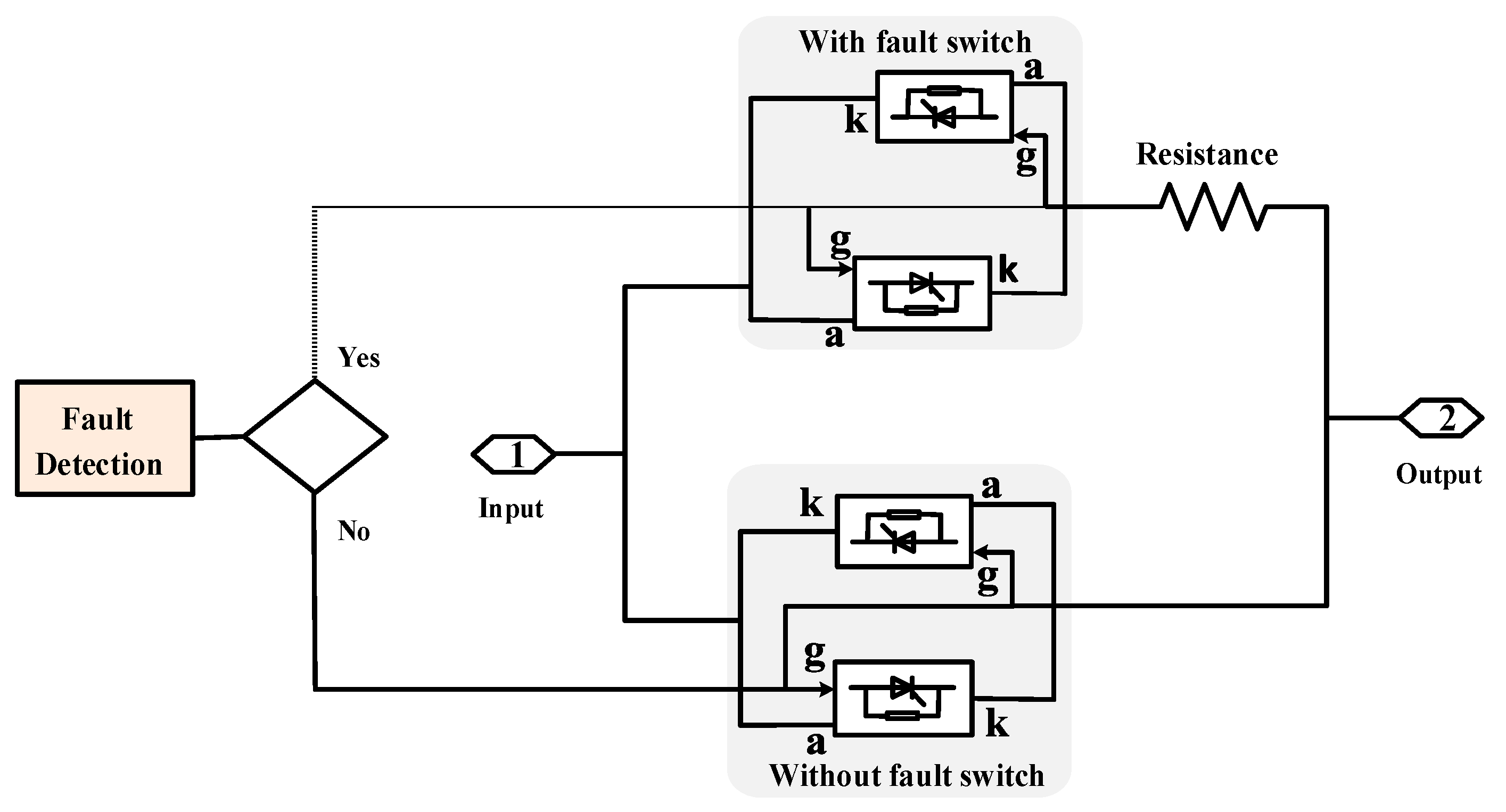
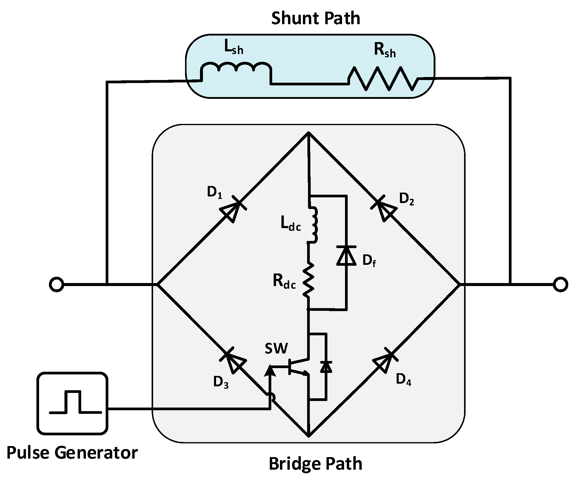
Bridge-Type Fault Current Limiters (BFCL)

The BFCL strategy for LVRT enhancement of rotating units like doubly fed induction generator (DFIG) has been proposed [40]. To analyze and investigate the response of BFCL for grid-connected PVS to enhance its LVRT capability for the grid requirement is proposed here. The fault currents are optimized to rated values without compromising at ripples by the BFCL strategy through its dual path control.

The BFCL strategy is comprised of two paths i.e., bridge path and shunt path [41]. The bridge path using the current in normal conditions, which consists of four diodes (D₁-D₄) connected to pass both the positive and negative half cycles of alternating current. The parallel connected small DC-reactor (${\mathrm{L}}_{\mathrm{dc}}$) and a freewheeling diode (${\mathrm{D}}_{\mathrm{f}}$) are come in series with a power electronic switch, as depicted from Figure 7. A very small amount of resistance is included as an inductor inheritance resistance (${\mathrm{R}}_{\mathrm{dc}}$). The shunt path is a series branch of an inductor (${\mathrm{L}}_{\mathrm{sh}}$) and a resistor (${\mathrm{R}}_{\mathrm{sh}}$), which is parallel with the bridge path.

The BFCL circuitry operates in such a way that, during normal conditions, the power electronic switch of the bridge path remains triggered to keep it closed for power flow. The path ${\mathrm{D}}_1$-${\mathrm{L}}_{\mathrm{dc}}$. -${\mathrm{R}}_{\mathrm{dc}}$-${\mathrm{D}}_4$ passes one-half cycle of the alternating current. However, ${\mathrm{D}}_2$-${\mathrm{L}}_{\mathrm{dc}}$-${\mathrm{R}}_{\mathrm{dc}}$-${\mathrm{D}}_3$ passes another half cycle. During abnormal conditions, the bridge path becomes open and power flow is diverted to the high impedance path i.e., shunt path to limit high fault currents. Due to the abrupt increase in current during fault initiation, the reactor ${\mathrm{L}}_{\mathrm{dc}}$ limits the high $\raisebox{1ex}{$\mathrm{di}$}\!\left/ \!\raisebox{-1ex}{$\mathrm{dt}$}\right.$ changes to assure safe operation of the switch.

For design consideration, the BFCL circuit should consume power equal to that of the line carries at the pre-fault to save the system from high disturbances. Equation (21) and Equation (22) give power consumed by BFCL during the post-fault as:

$${\mathrm{P}}_{\mathrm{BFCL}}\le \frac{{\mathrm{P}}_{\mathrm{gen}}}{2}$$

(21)

$${\mathrm{P}}_{\mathrm{BFCL}}=\frac{{\mathrm{V}}_{\mathrm{PCC}}^2{\mathrm{R}}_{\mathrm{sh}}}{{\mathrm{R}}_{\mathrm{sh}}^2+{\mathrm{X}}_{\mathrm{sh}}^2}$$

(22)

In this case, ${\mathrm{P}}_{\mathrm{gen}}$, ${\mathrm{V}}_{\mathrm{PCC}}$, and ${\mathrm{X}}_{\mathrm{sh}}$ are the power-generated voltage at PCC and shunt inductance, respectively. By substituting Equation (22) into Equation (21), the inequality becomes:

$${\mathrm{R}}_{\mathrm{sh}}\ge \frac{{\mathrm{V}}_{\mathrm{PCC}}^2+\sqrt{{\mathrm{V}}_{\mathrm{PCC}}^4-{\mathrm{P}}_{\mathrm{gen}}^2{\mathrm{X}}_{\mathrm{sh}}^2}}{{\mathrm{P}}_{\mathrm{gen}}}$$

(23)

The condition for ${\mathrm{R}}_{\mathrm{sh}}$ to be a real number is shown below.

$$X_{sh}<\frac{{\mathrm{V}}_{\mathrm{PCC}}^2}{{\mathrm{P}}_{\mathrm{gen}}}$$

(24)

Following this condition for shunt reactance, a smooth and ripple-free optimized current waveform of fault current can be achieved.

3. Results and Discussion

The platform used for implementation of the 100-kW 3-phase grid connected to the photovoltaic system is Matlab/Simulink. The effect of fault parameters for the system are investigated for designed FLC based on the LM and BFCL-based FRT strategy. The response of fault parameters at both grids as well as the PV side are analyzed at two locations i.e., PCC and at 5-km of distance from PCC. Moreover, for justification of the proposed control, a comparative assessment is carried out with conventionally tuned PI and crowbar based FRT strategy.

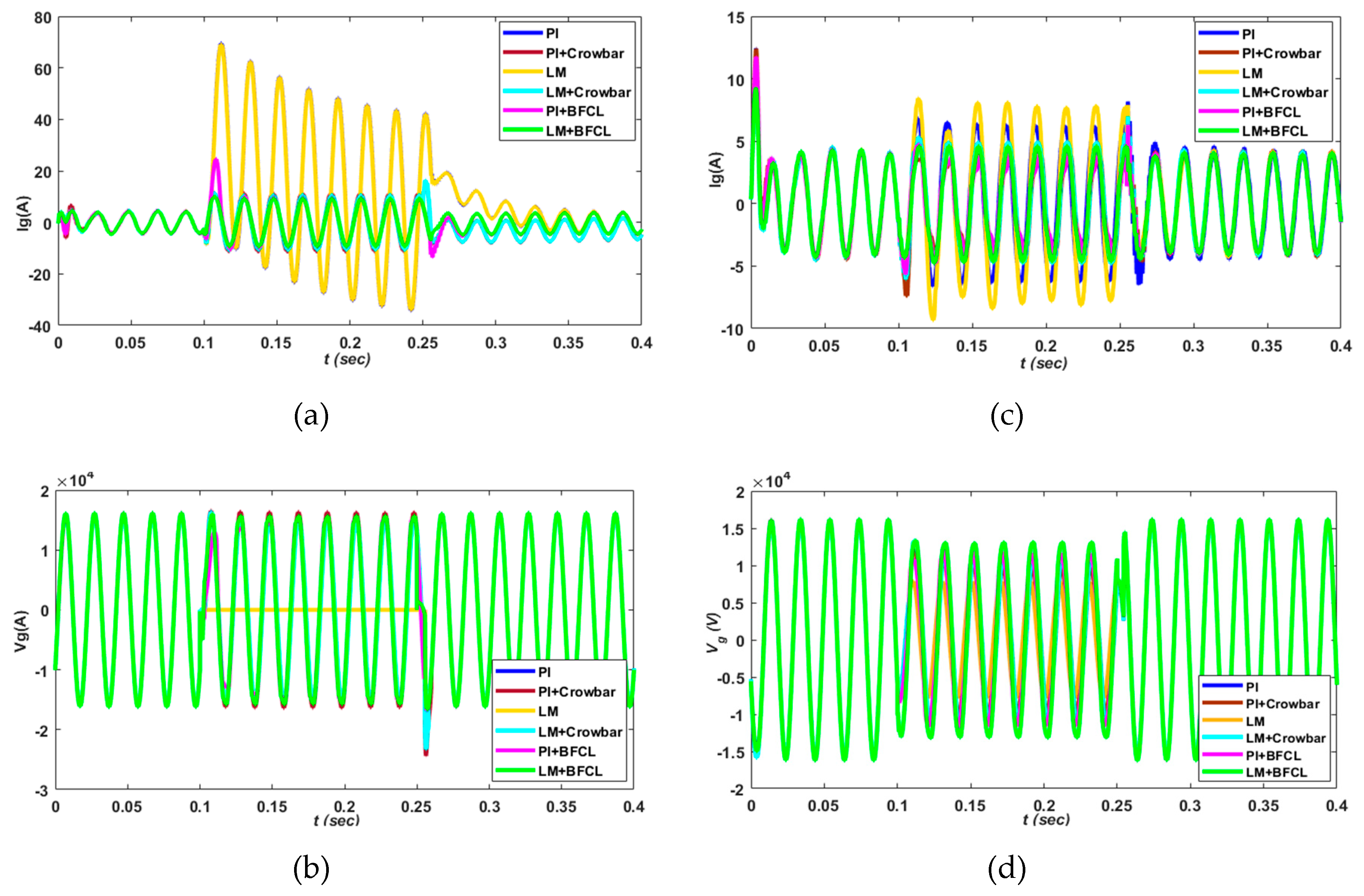
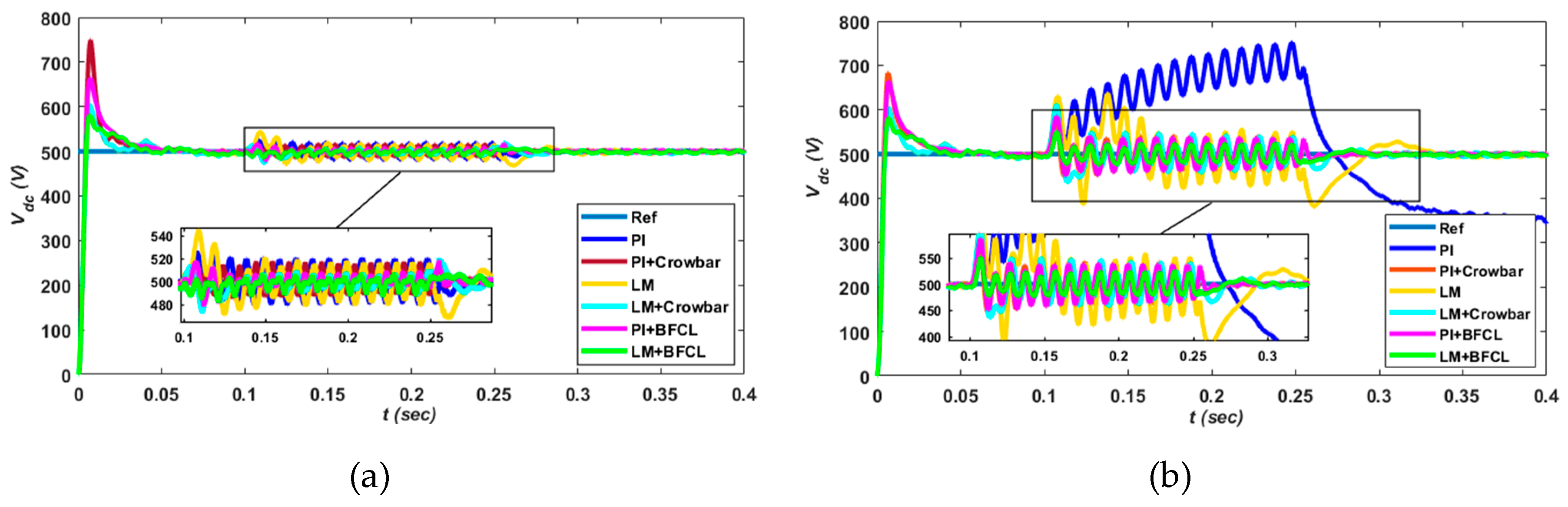
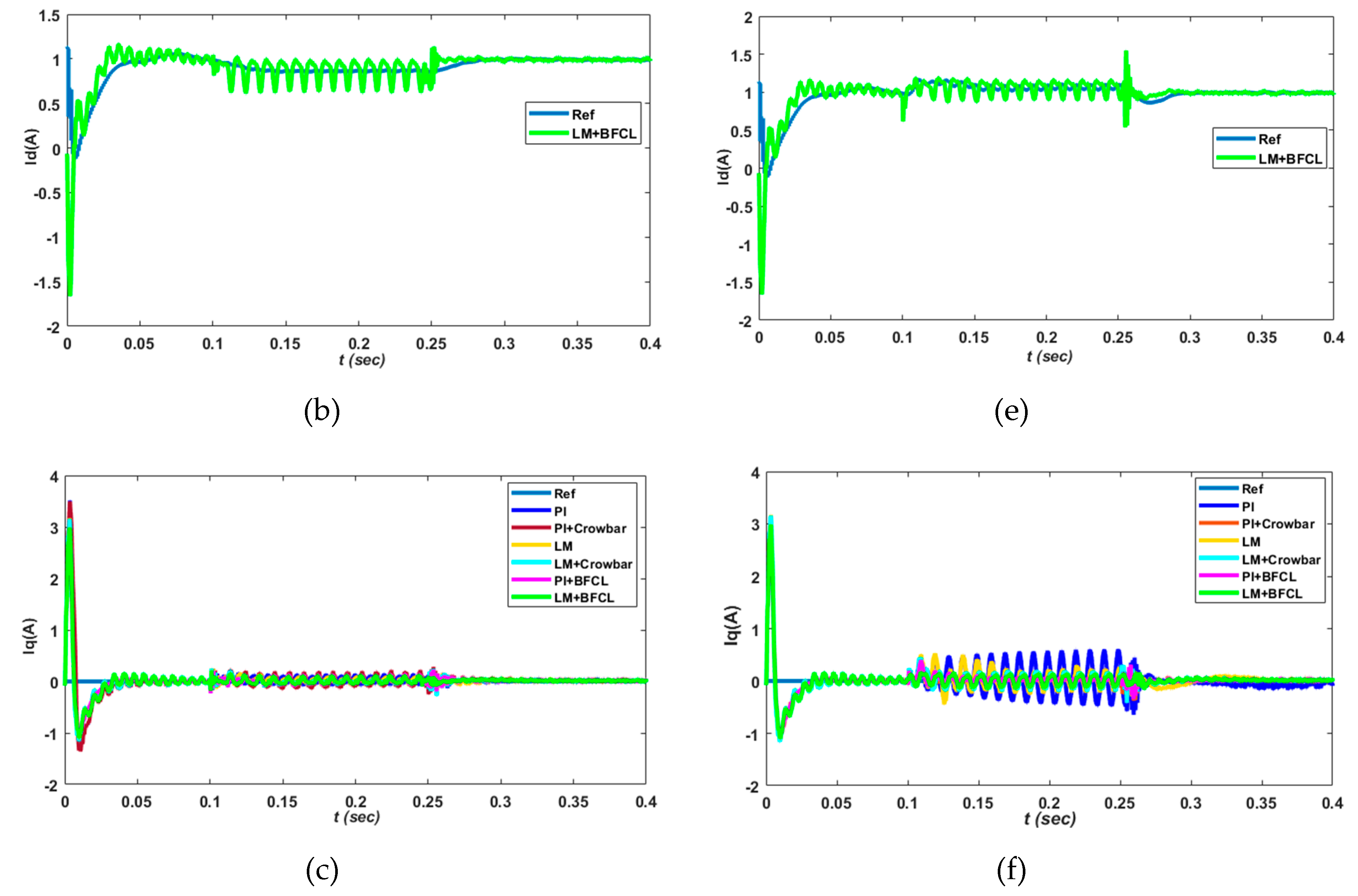
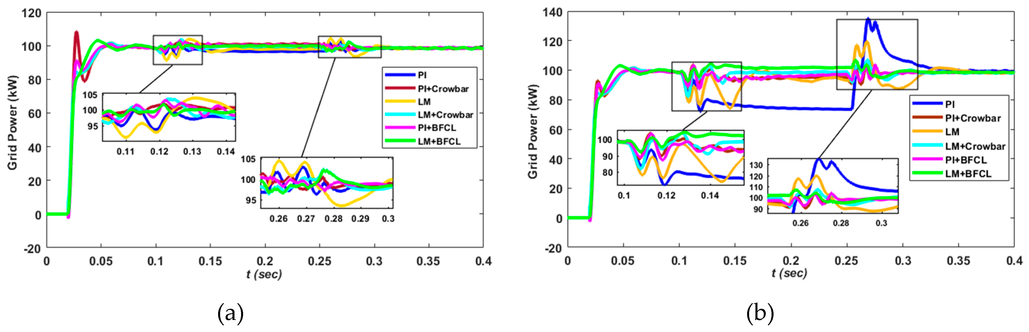
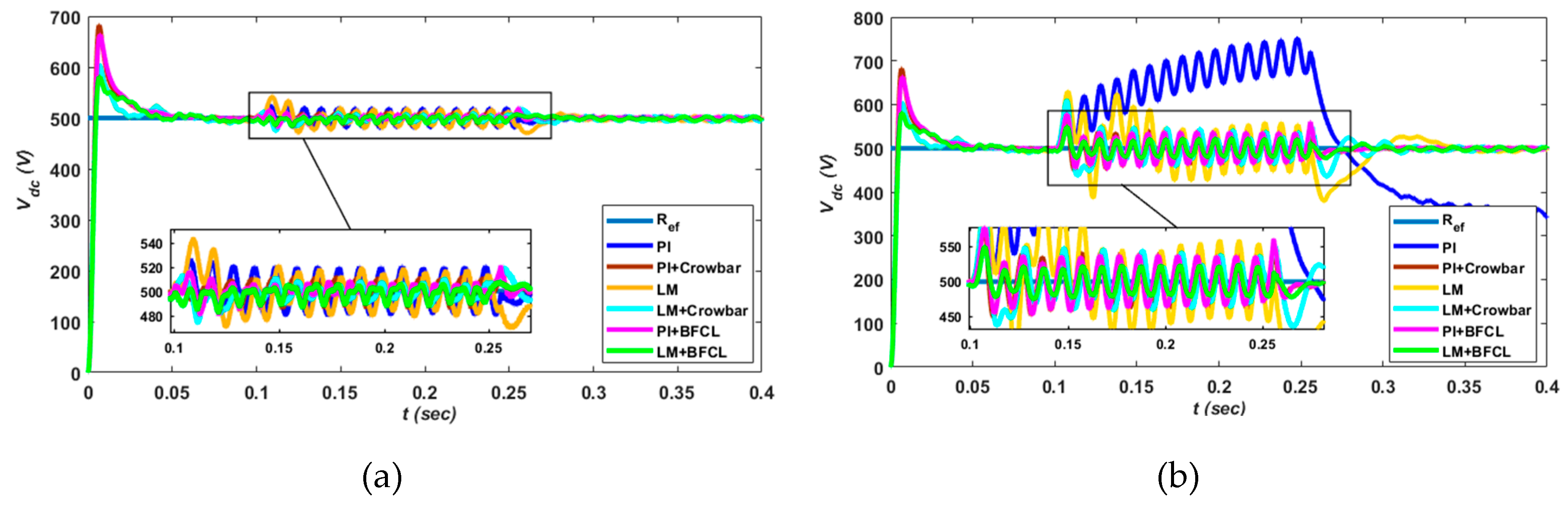
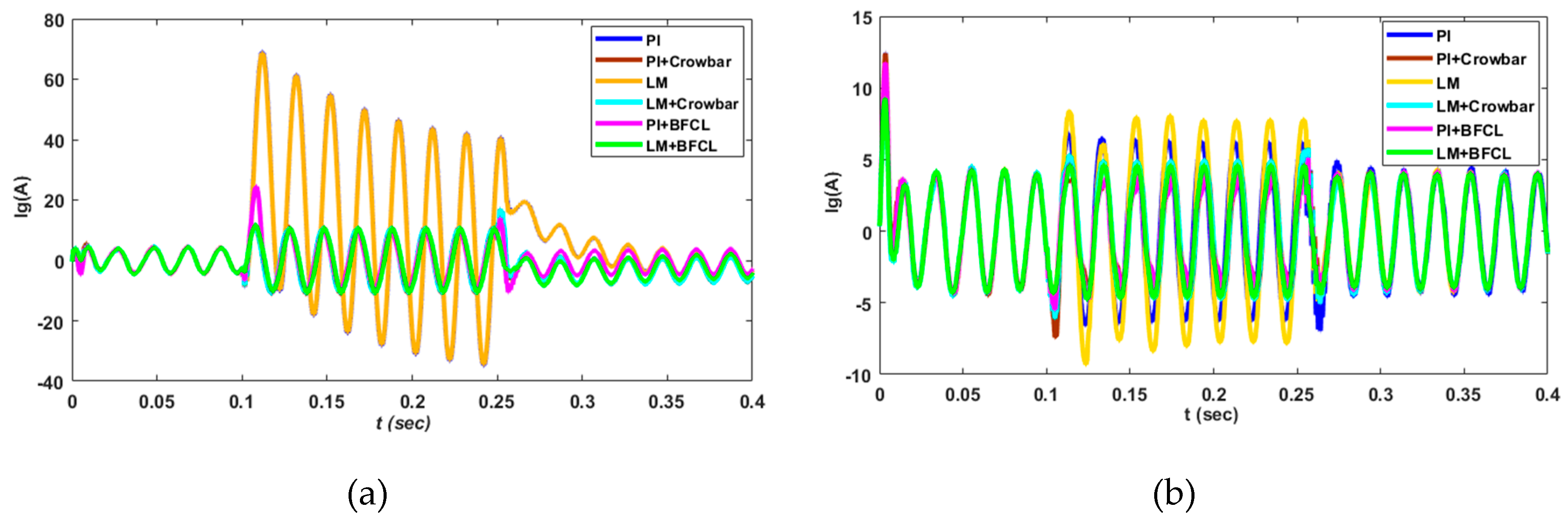
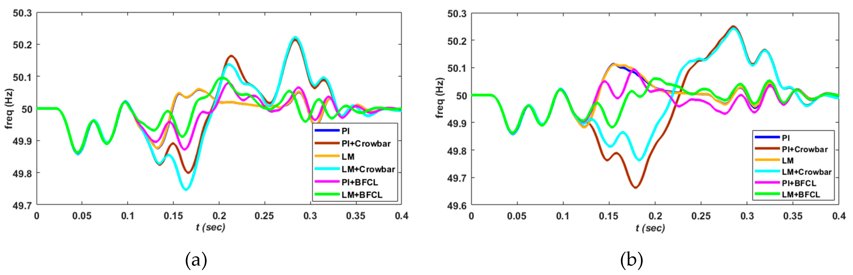
3.1. Asymmetrical Faults at PCC

Asymmetrical faults are applied at 0.1 s for 150 ms at PCC. Performance analysis of the proposed approach in comparison with conventionally used schemes is presented below.

The DC-link voltage behavior during the phase to the ground (P-G) and phase-to-phase (P-P) faults are depicted in Figure 8. The proposed BFCL in combination with FLC based on LM (LM+BFCL) shows a smooth and optimized response throughout the fault duration. The proposed strategy gives minimum spikes at the fault occurring and clearing the time. It also responds with a minimum overshoot and undershoot as compared to any of the other approaches. However, the double phase fault responds more severely as compared to a single-phase fault. However, the response of the proposed strategy justifies its robustness for the P-P fault as well. Moreover, during the start of simulations, LM+BFCL responds in minimum transients, comparatively.

Additionally, the contents of

Table 1. Performance index analysis of the Designed Control Scheme for Vdc.

Control Strategies	Single Phase			Two Phase
	IAE	ISE	ITAE	IAE	ISE	ITAE
PI	0.0211	0.43	0.0029	0.0754	1.233	0.0161
PI+Crowbar	0.0158	0.38	0.0025	0.0185	0.924	0.0029
LM	0.0266	0.52	0.0031	0.0612	1.145	0.0131
LM+Crowbar	0.0143	0.56	0.0020	0.0184	0.839	0.0024
PI+BFCL	0.0126	0.48	0.0007	0.0629	0.953	0.0018
LM+BFCL	0.0122	0.46	0.0006	0.0158	0.872	0.0013

Integral-Absolute-Error (IAE), Integral-Square-Error (ISE), and Integral of Time-Weighted-Absolute-Error (ITAE).

,

Table 2. Performance index analysis of the Designed Control Scheme for Id.

Control Strategies	Single Phase			Two Phase
	IAE	ISE	ITAE	IAE	ISE	ITAE
PI	0.0357	0.0096	0.0051	0.1164	0.0500	0.0290
PI + Crowbar	0.1107	0.0633	0.0269	0.1204	0.0755	0.0296
LM	0.0273	0.0061	0.0041	0.1424	0.0833	0.0354
LM + Crowbar	0.0935	0.0405	0.0228	0.1030	0.0496	0.0257
PI + BFCL	0.0338	0.0110	0.0042	0.1114	0.0486	0.0278
LM + BFCL	0.0258	0.0071	0.0030	0.1002	0.0412	0.0257

Integral-Absolute-Error (IAE), Integral-Square-Error (ISE), Integral of Time-Weighted-Absolute-Error (ITAE).

and

Table 3. Performance index analysis of the designed control scheme for Iq.

Control Strategies	Single Phase			Two Phase
	IAE	ISE	ITAE	IAE	ISE	ITAE
PI	0.0426	0.0513	0.0028	0.0834	0.0672	0.0113
PI + Crowbar	0.0655	0.0574	0.0096	0.0746	0.0601	0.0113
LM	0.0434	0.0516	0.0027	0.0997	0.0931	0.0142
LM + Crowbar	0.0531	0.0531	0.0053	0.0826	0.0557	0.0090
PI + BFCL	0.0371	0.0368	0.0021	0.0747	0.0490	0.0099
LM + BFCL	0.0321	0.0392	0.0019	0.0734	0.0485	0.0087

Integral-Absolute-Error (IAE), Integral-Square-Error (ISE), Integral of Time-Weighted-Absolute-Error (ITAE).

elaborates the control measures to evaluate the performance of different control schemes. Three control measures i.e., Integral Absolute Error (IAE), Integral Square Error (ISE), and Integral Time-weighted Absolute Error (ITAE) are calculated. These measures give a very precise and exact comparison between the different controllers. The minimum is the value while the more is the efficiency.

Performance evaluations of the proposed strategy for the dc-link voltage with other possible combinations are carried out in Table 1.

Figure 9 depicts the inverter active (Id) and reactive (Iq) current components in the synchronous reference frame i.e., d-q frame. In both the unbalanced fault conditions P-G and P-P, the proposed scheme authenticates the low oscillations and surges in currents. This is due to the inductive effect of BFCL comparatively to crowbar as the FRT strategy. Furthermore, the P-P fault proposed scheme gives an optimum response even though it is a severe fault than the P-G fault. However, as mentioned before, the Iq component is kept at zero for the unity power factor. Therefore, the Iq component also proposed LM+BFCL, which gives negligible spikes for both fault cases, as shown in Figure 9c,f. Additionally, most of the performance evaluation indices give minimum values for the proposed approach, as shown in Table 2; Table 3. The minimum value of adopted performance evaluation indices means efficient performance.

Performance evaluation of the proposed strategy with other possible combinations are derived in Table 2 for the real current component (Id).

However, performance evaluations for a reactive current component for all possible combinations are carried out in Table 3.

Figure 10 shows the propagation of real power waveforms during unbalanced short circuit faults. These faults are simulated at the PCC of PVS, which is measured through 100 kVA power rating and 260V/20kV coupling transformer. Both of the controllers i.e., PI and LM alone results in the worst behavior. Approximately 8% and 20% of power dips occurred during P-G and P-P, respectively, along with extensively high transition surges. However, with the combination of crowbar circuitry, an increase in power is achieved but with high and long duration oscillations during the fault occurring and clearing time. The proposed LM+BFCL results in rated power during the fault without compromising at high oscillations and surges, as shown by Figure 10a,b for single phase and double phase abnormal conditions.

The fault current waveforms are substantially restrained to acceptable limits through a proposed strategy, and loss of voltage is regained to a rated value without any ripples during the P-G fault as shown in Figure 11. However, the crowbar strategy with any of the controllers restricts current due to its pure resistive effect but results in high spikes during the fault occurring and clearing time. During the P-P fault, the proposed strategy gives a smooth and optimized response due to shunt inductance during the fault and bridge inductance for switching surge elimination.

Furthermore, total harmonic distortion (THD) is calculated with fast Fourier transform (FFT) analysis for grid current and voltage during the P-G fault. The distortion in harmonics is carried out under analysis for a proposed approach (LM+BFCL) and for other possible combinations i.e., from Figure 12, Figure 13, Figure 14, Figure 15, Figure 16 and Figure 17. The proposed approach gives minimum values of THD for current and voltage i.e., 16.24% and 9.20%, respectively, as depicted by Figure 17. However, for the conventionally adopted PI + Crowbar strategy, the THD values 24.79% and 15.46% for the current and voltage are depicted in Figure 13.

However, considering the THD response of controllers without FRT strategy i.e., for PI and FLC based on LM optimization. The LM optimization-based control have 21% and 112.63% THD for current and voltage, respectively. However, the conventional PI controller results in 24.95% and 175.08% for current and voltage, respectively, as shown by Figure 12 and Figure 13. Therefore, the minimum percent value of THD for LM optimization-based control shows low harmonics as compared to a conventionally tuned PI controller. According to overall harmonics analysis, it is clearly authenticated that the proposed approach is more efficient and have low harmonics distortion than all possible combinations of controllers and FRT strategies.

The frequency variations during P-G and P-P are depicted in Figure 18. According to the German grid code, the frequency variation limits for normal operation are 49.5-50.5 Hz for 50 Hz nominal frequency. However, for serious contingency, the critical frequency variations are 47.0-48.0 Hz for 50 Hz nominal frequency [42,43]. Therefore, each of the presented schemes is obeying the frequency requirements of grid codes. The crowbar strategy results in high variations. However, proposed LM+BFCL gives minimum variations for P-G faults as shown by Figure 18a. In the case of the P-P fault, frequency responds in high amplitude variations than the P-G fault for the crowbar FRT strategy, as shown by Figure 18b. However, for both fault cases, the smooth and optimum response of the proposed approach is authenticated.

The impact of faults on PV array output power results in a decrease at the fault occurring and clearance time. This decrease in power is more significant for the P-P fault whereas, for the P-G fault, it varies little. Considering the performance of FRT schemes, Figure 19a,b clearly show a smooth and fast response for the proposed strategy in both cases of the fault. Yet, with other schemes, a decrease in PV power is faced for 0.04 s as the fault transients, which is more significant with the crowbar strategy due to its pure resistive nature. This is why it results in a high copper loss (${\mathrm{I}}^2\mathrm{R}$).

The PV array current and voltage wave forms during single phase and double phase fault are shown in Figure 20. Both current and voltage give high magnitude surges during fault occurring and clearing time, which are higher for the P-P fault and less for the P-G fault. The instantaneous product of voltage and current in both fault cases justifies the PV power waveform, as shown in Figure 19, according to the power law i.e., P = V*I. Moreover, the proposed strategy authenticates its optimum response comparatively to other schemes in PV output power.

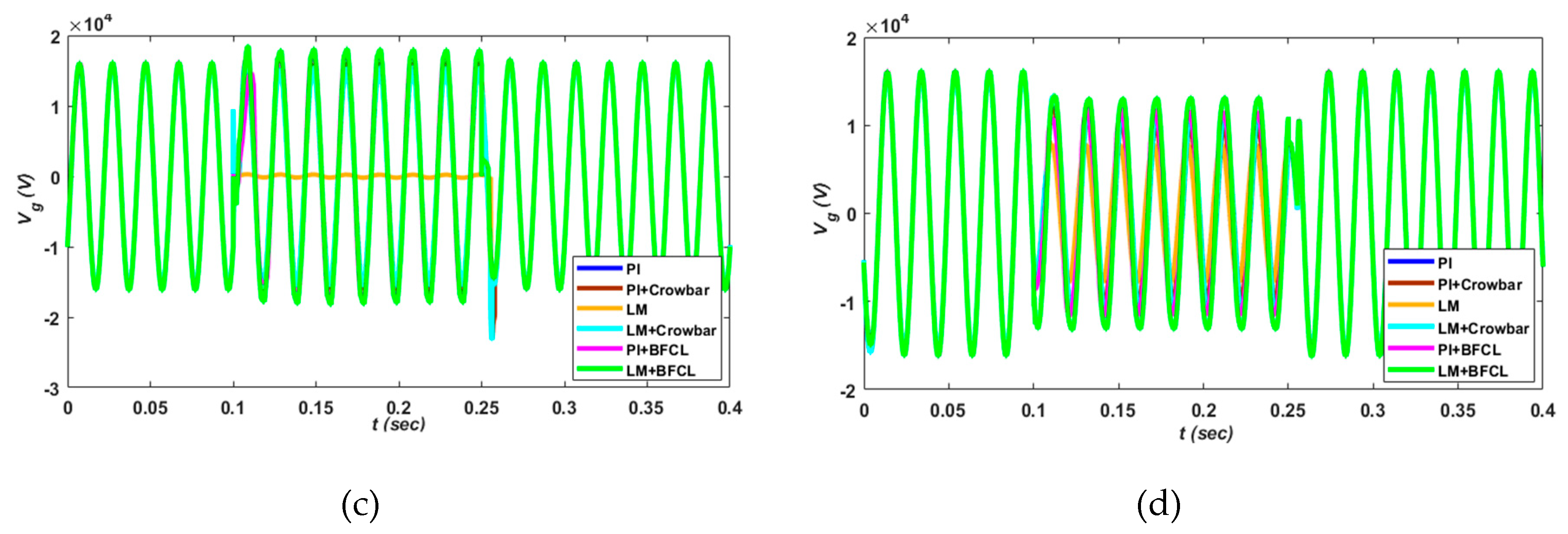
3.2. Asymmetrical Faults at 5-km Distance

The simulated parameters at 5-km from PCC influenced little more than the type of fault rather than the distance. The small variations with respect to distance are due to the addition of extra 5-km line impedance. A negligible increase in voltage waveforms and a decrease in current waveforms are depicted even though the overall behavior is the same as in PCC.

The DC-link voltage response during the P-G and P-P fault at the 5-km distribution line from PCC is shown in Figure 21a,b, respectively, which results in small variations throughout fault time due to the line impedance. Line distance does not alter the effectiveness of the proposed strategy as compared to other schemes.

Figure 22 clarifies the low amplitude oscillations in active (Id) and reactive (Iq) current components for the proposed LM + BFCL strategy during both unbalanced conditions. Yet, insignificant increases in spikes are observed due to line impedance for the conventional crowbar with the PI controller as compared to that of PCC. However, the proposed strategy results in more surge suppression due to line series impedance and shunt impedance of the BFCL strategy.

The small decrease in current and increase in grid voltage due to faults at 5-km of distance from PCC are shown in Figure 23. Same as in PCC, grid currents and voltages at 5-km away abnormalities result in spikes and ripples with conventional crowbar circuitry.

The frequency response is approximately the same as in PCC since frequency is independent of line resistance, which is shown by Figure 24 for asymmetrical faults at the 5-km distance of the distribution line.

Moreover, the grid side parameters like PV power, current, and voltage authenticates the efficiency of the proposed methodology even at fault at the distribution line. However, negligible variations are there but these variations are for all combinations of presented schemes and the power law justifies in this case, as discussed for faults in PCC. The simulated responses of PV parameters at P-G and P-P faults at 5-km of distance from PCC are given by Figure 25 below.

4. Conclusions

This paper emphasizes enhancement of LVRT capability of the three-phase grid connected PVS, according to the existing grid requirements during unbalanced faults. The proposed strategy BFCL in coordination with FLC based on LM optimization (LM+BFCL) is successfully analyzed and compared with a conventionally adopted crowbar strategy and an optimally tuned PI controller. A promising response is accomplished at both sides of PVS i.e., grid side and PV side at two locations such as at PCC and at 5-km distance from PCC. Moreover, it is analyzed that the impact on variables of grid-connected PVS are less influenced with respect to distance and more influenced due to fault type.

The performance evaluation indices i.e., IAE, ITAE, and ISE and THD analysis effectively validates the improvement of the dc-link voltage, power, voltage, and current. Additionally, the proposed approach authenticates smooth, fast, robust, and a fault tolerant response under normal conditions and fault conditions. In the near future, the designed control scheme will be extended by adopting new designed strategies like Feedback Linearization, Adaptive L1, High Order Adaptive SMC, and H-infinity. Furthermore, the proposed scheme will be experimentally validated using the Delfino Texas Instrument or DSP (TMS3200F28335) boards.

References

1. Willisand, H.L.; Scott, W.G. Distributed Power Generation: Planning and Evaluation; Marcel-Dekker: New York, NY, USA, 2000. [Google Scholar]
2. Dvarioniene, J.; Sinkuniene, J.; Gurauskiene, I.; Gecevicius, G.; Stasiskiene, Z. Analysis of integration of solar collector systems into district heat supply networks. Environ. Eng. Manag. J. 2013, 12, 2041–2050. [Google Scholar] [CrossRef]
3. Available online: http://www.iea-pvps.org/fileadmin/dam/public/report/statistics/PVPS_report_-_A_Snapshot_of_Global_PV_-_1992-2013_-_final_3.pdf (accessed on 3 January 2019).
4. Javadi, M.; Marzband, M. A Centralized Smart Decision-Making Hierarchical Interactive Architecture for Multiple Home Microgrids in Retail Electricity Market. Energies 2018, 11, 3144. [Google Scholar] [CrossRef]
5. Valinejad, J.; Marzband, M. Long-term decision on wind investment with considering different load ranges of power plant for sustainable electricity energy market. Sustainability 2018, 10, 3811. [Google Scholar] [CrossRef]
6. Masson, G.; Latour, M.; Rekinger, M.; Theologitis, I.T.; Papoutsi, M. Global Market Outlook for Photovoltaics 2013–2017; EUIP: Brussels, Belgium, 2013. [Google Scholar]
7. REN21. Renewables 2014: Global Status Report. pp. 15–16. 2014. Available online: http://www.webcitation.org/6SKF06GAX (accessed on 8 February 2019).
8. Valinejad, J.; Barforoshi, T.; Marzband, M. Investment Incentives in Competitive Electricity Markets. Appl. Sci. 2018, 8, 1978. [Google Scholar] [CrossRef]
9. Marzband, M.; Azarinejadian, F. Smart transactive energy framework in grid-connected multiple home microgrids under independent and coalition operations. Renew. Energy 2018, 126, 95–106. [Google Scholar] [CrossRef]
10. Bueno, P.G.; Hernández, J.C. Stability assessment for transmission systems with large utility-scale photovoltaic units. IET Renew. Power Gener. 2016, 10, 584–597. [Google Scholar] [CrossRef]
11. Ruiz-Rodriguez, F.J.; Hernández, J.C. Voltage unbalance assessment in secondary radial distribution networks with single-phase photovoltaic systems. Int. J. Electr. Power Energy Syst. 2015, 64, 646–654. [Google Scholar] [CrossRef]
12. Iov, F.; Hansen, A.D.; Sørensen, P.E.; Cutululis, N.A. Mapping of Grid Faults and Grid Codes; Risø National Laboratory, Technical University of Denmark: Roskilde, Denmark, 2007. [Google Scholar]
13. On-GmbH, E. Grid Code—High and Extra High Voltage. Available online: http://www.eon-netz.com/ (accessed on 27 January 2019).
14. Braun, M.; Arnold, G.; Laukamp, H. Plugging into the Zeitgeist. IEEE Power Energy Mag. 2009, 7, 63–76. [Google Scholar] [CrossRef]
15. Comitato Elettrotecnico Italiano. CEI0-21: Reference Technical Rules for Connecting Users to the Active and Passive LV Distribution Companies of Electricity. Available online: http://www.ceiweb.it/ (accessed on 4 January 2019).
16. Altin, M.; Goksu, O.; Teodorescu, R.; Rodriguez, P.; Jensen, B.B.; Helle, L. Overview of recent grid codes for wind power integration. In Proceedings of the 12th International Conference on Optimization of Electrical and Electronic Equipment, Brasov, Romania, 20–22 May 2010; pp. 1152–1160. [Google Scholar]
17. Beach, T.; Kozinda, A.; Rao, V. Advanced Inverters for Distributed PV: Latent Opportunities for Localized Reactive Power Compensation; NREL/BR-6A20-62612; Cal x Clean Coalition Energy: Menlo Park, CA, USA, 2013; p. C226. Available online: https://clean-coalition.org/wp-content/uploads/2018/12/A.14-11-016-Ex-Parte-Letter-from-Clean-Coalition-in-support-of-DeAngelis-Proposed-Decision-with-attachments.pdf (accessed on 7 January 2019).
18. Ding, G.; Gao, F.; Tian, H.; Ma, C.; Chen, M.; He, G.; Liu, Y. Adaptive dc-link voltage control of two-stage photovoltaic inverter during low voltage ride-through operation. IEEE Trans. Power Electron. 2016, 31, 4182–4194. [Google Scholar] [CrossRef]
19. Stetz, T.; Marten, F.; Braun, M. Improved low voltage grid-integration of photovoltaic systems in Germany. IEEE Trans. Sustain. Energy 2013, 4, 534–542. [Google Scholar] [CrossRef]
20. Tsili, M.; Papathanassiou, S. A review of grid code technical requirements for wind farms. IET Renewable Power Gener. 2009, 3, 308–332. [Google Scholar] [CrossRef]
21. Troester, E. New German grid codes for connecting PV systems to the Medium Voltage Power Grid, 2nd; In Proceedings of the International Workshop on Concentrating PV Power Plants, Darmstadt, Germany, 18 November 2011.
22. Lin, W.M.; Hong, C.M. A new Elman neural network-based control algorithm for adjustable-pitch variable-speed wind-energy conversion systems. IEEE Trans. Power Electron. 2011, 26, 473e481. [Google Scholar] [CrossRef]
23. Gaing, Z.L. Wavelet-based neural network for power disturbance recognition and classification. IEEE Trans. Power Del. 2004, 19, 1560e1568. [Google Scholar] [CrossRef]
24. Rodriguez, P.; Timbus, A.V.; Teodorescu, R.; Liserre, M.; Blaabjerg, F. Flexible active power control of distributed power generation systems during grid faults. IEEE Trans. Ind. Electron. 2007, 54, 2583–2592. [Google Scholar] [CrossRef]
25. Teodorescu, R.; Liserre, M.; Rodriguez, P. Grid Converters for Photovoltaic and Wind Power Systems; Wiley: Hoboken, NJ, USA, 2011; Volume 29. [Google Scholar]
26. Castilla, C.M.; Miret, J.; Borrell, A.; de Vicuna, L.G. Active and reactive power strategies with peak current limitation for distributed generation inverters during unbalanced grid faults. IEEE Trans. Ind. Electron. 2015, 62, 1515–1525. [Google Scholar]
27. Specht, D.F. Probabilistic neural network. Neural Netw. 1990, 3, 109–118. [Google Scholar] [CrossRef]
28. Liu, Z.; Li, H.X. A probabilistic fuzzy logic system for modeling and control. IEEE Trans. Fuzzy Syst. 2005, 13, 848–859. [Google Scholar]
29. Cardenas, R.; Pena, R.; Alepuz, S.; Asher, G. Overview of control system for the operation of DFIGs in wind energy application. IEEE Trans. Ind. Electron. 2013, 60, 2776–2798. [Google Scholar] [CrossRef]
30. Li, H.X.; Liu, Z. A probabilistic neural-fuzzy learning system for stochastic modeling. IEEE Trans. Fuzzy Syst. 2008, 16, 898e908. [Google Scholar] [CrossRef]
31. Zeb, K.; Khan, I.; Uddin, W. A Review on Recent Advances and Future Trends of Transformerless Inverter Structures for Single-Phase Grid-Connected Photovoltaic Systems. Energies 2018, 11, 1968. [Google Scholar] [CrossRef]
32. Massawe, H.B. Grid Connected Photovoltaic Systems with SmartGrid functionality. Master’s Thesis, Norwegian University of Science and Technology, Trondheim, Norway, 2013. [Google Scholar]
33. Makhlouf, M.; Messai, F.; Benalla, H. Modeling and control of a single-phase grid connected photovoltaic system. J. Theor. Appl. Inf. Technol. 2012, 37, 289–296. [Google Scholar]
34. Available online: www.mathworks.com (accessed on 27 February 2019).
35. Banu, V.; Istrate, M. Modeling of maximum power point tracking algorithm for PV systems. In Proceedings of the 7th International Conference and Exposition on Electrical and Power Engineering (EPE), Lasi, Romania, 25–27 October 2012; pp. 953–957. [Google Scholar]
36. Kazmierkowski, M.; Krishnan, R.; Blaabjerg, F. Control in Power Electronics—Selected Problems; Academic Press: New York, NY, USA, 2002. [Google Scholar]
37. Harb, A.M.; Smadi, I.A. An Approach to Fuzzy Control for a Class of Nonlinear Systems: Stability and Design Issues. Int. J. Model. Simul. 2015, 25, 106–111. [Google Scholar] [CrossRef]
38. Wilamowski, B.M.; Yu, H. Im proved computation for Levenberg Marquardt training. IEEE Trans. Neural Netw. 2010, 21, 930–937. [Google Scholar] [CrossRef] [PubMed]
39. Menhaj, M.T.H.M. Training feedforward networks with the Marquardt algorithm. IEEE Trans. Neural Netw. 1994, 5, 989–993. [Google Scholar]
40. Rashid, G.; Hasan Ali, M. Transient Stability Enhancement of Doubly Fed Induction Machine-Based Wind Generator by Bridge-Type Fault Current Limiter. IEEE Trans. Energy Convers. 2015, 30, 939–947. [Google Scholar] [CrossRef]
41. Naderi, S.B.; Jafari, M. Impact of bridge type fault current limiter on power system transient stability. In Proceedings of the 7th International Conference of Electronic Engineering, Bursa, Turkey, 4 December 2011; pp. 1–4. [Google Scholar]
42. Luo, X.; Wang, J. Review of Voltage and Frequency Grid Code Specifications for Electrical Energy Storage Applications. Energies 2018, 11, 1070. [Google Scholar] [CrossRef]
43. Hernández, J.C.; Bueno, P.G. Enhanced utility-scale photovoltaic units with frequency support functions and dynamic grid support for transmission systems. IET Renew. Power Gener. 2017, 11, 361–372. [Google Scholar] [CrossRef]
Figure 1. Equivalent circuit of PV cell.
Electronics 08 00429 g001
Figure 2. Equivalent circuit of the boost converter.
Electronics 08 00429 g002
Figure 3. Proposed model for three-phase grid-connected PVS.
Electronics 08 00429 g003
Figure 4. The control scheme for the grid-connected inverter.
Electronics 08 00429 g004
Figure 5. FLC based on the LM optimization algorithm.
Electronics 08 00429 g005
Figure 6. Crowbar circuit with controlled switches.
Electronics 08 00429 g006
Figure 7. BFCL circuitry.
Electronics 08 00429 g007
Figure 8. DC-link voltage response for P-G 8 (a) and P-P 8 (b) at PCC.
Electronics 08 00429 g008
Figure 9. Active (Id), reactive (Iq) currents in 9 (a, b, c) and 9 (d, e, f) during P-G and P-P fault, respectively.
Electronics 08 00429 g009aElectronics 08 00429 g009b
Figure 10. Grid real power response during the P-G fault 10(a) and P-P fault 10(b).
Electronics 08 00429 g010
Figure 11. Grid currents and voltage during P-G 11 (a, b) and P-P 11 (c, d), respectively.
Electronics 08 00429 g011
Figure 12. THD with PI controller for grid current (a) and voltage (b) during the P-G fault.
Electronics 08 00429 g012
Figure 13. THD with PI + Crowbar scheme for grid current (a) and voltage (b) during the P-G fault.
Electronics 08 00429 g013
Figure 14. THD with LM controller for grid current (a) and voltage (b) during the P-G fault.
Electronics 08 00429 g014
Figure 15. THD with LM + Crowbar scheme for grid current (a) and voltage (b) during the P-G fault.
Electronics 08 00429 g015
Figure 16. THD with PI + BFCL scheme for grid current (a) and voltage (b) during the P-G fault.
Electronics 08 00429 g016
Figure 17. THD with LM + BFCL scheme for grid current (a) and voltage (b) during the P-G fault.
Electronics 08 00429 g017
Figure 18. Frequency variations in PCC during the P-G fault 18(a) and P-P fault 18(b).
Electronics 08 00429 g018
Figure 19. PV array power during the P-G fault 19(a) and the P-P fault 19(b) at PCC.
Electronics 08 00429 g019
Figure 20. Current and voltage of PV array during P-G 20 (a, b) and P-P fault 20 (c, d) at PCC.
Electronics 08 00429 g020
Figure 21. DC-link voltage during P-G fault 21 (a) and P-P fault 21 (b) at 15-km from PCC.
Electronics 08 00429 g021
Figure 22. Active (Id) and reactive (Iq) current components during P-G (a, b, c) and P-P (d, e, f) at 5-km distance.
Electronics 08 00429 g022
Figure 23. Grid current and voltage during the P-G fault (a, b) and the P-P fault (c, d) at 5-km from PCC.
Electronics 08 00429 g023aElectronics 08 00429 g023b
Figure 24. Frequency behavior during the P-G fault (a) and the P-P fault (b) at 5-km distance from PCC.
Electronics 08 00429 g024
Figure 25. PV output power, current, and voltage during the P-G fault (a, b, c) and the P-P fault (d, e, f), respectively, at 5 km.
Electronics 08 00429 g025aElectronics 08 00429 g025b