Comparison of Deep Learning and Conventional Demosaicing Algorithms for Mastcam Images


Abstract
1. Introduction
2. Demosaicing Algorithms and Performance Metrics
2.1. Algorithms
- Linear Directional Interpolation and Nonlocal Adaptive Thresholding (LDI-NAT): This algorithm is simple but the non-local search is time consuming [16].
- MHC: It is the Malvar–He–Cutler algorithm in [17]. This is the default method for demosaicing Mastcam images used by NASA. The algorithm is very efficient and simple to implement.
- Lu and Tan Interpolation (LT): It is from [24].
- Adaptive Frequency Domain (AFD): It is a frequency domain approach from Dubois [25]. The algorithm can also be used for other mosaicking patterns.
- Alternate Projection (AP): It is the algorithm from Gunturk et al. [26].
- Primary-Consistent Soft-Decision (PCSD): It is Wu and Zhang’s algorithm from [27].
- ATMF: This method is from [23]. At each pixel location, we demosaic pixels from seven methods; the largest and smallest pixels are removed and the mean of the remaining pixels are used. This method fuses the results from AFD, AP, LT, DLMMSE, MHC, PCSD, and LDI-NAT.
- Demosaicnet (DEMONET): In [19], a feed-forward network architecture was proposed for demosaicing. There are D + 1 convolutional layers and each layer has W outputs and uses K × K size kernels. An initial model was trained using 1.3 million images from Imagenet and 1 million images from MirFlickr. Additionally, some challenging images were searched to further enhance the training model. Details can be found in [19]. It should be noted that we have also performed some training using only Mastcam images. However, the customized model was not good as compared to the original one. This is probably due to lack of training data, as we have less than 100 high quality Mastcam images.
- Fusion using 3 best (F3) [22]: We only used F3 for Mastcam images. The mean of pixels from demosaiced images of LT, MHC, and LDI-NAT were used.
- Bilinear: We used bilinear interpolation for Mastcam images because it is the simplest algorithm.
- Deep Residual Network (DRL) [20]: A DRL algorithm is a deep learning based approach that was proposed for demosaicing based on a customized convolutional neural network (CNN) with a depth of 10 and a receptive field of size 21 × 21.
- Minimized-Laplacian Residual Interpolation (MLRI) [31]: This is a residual interpolation (RI)-based algorithm based on a minimized-Laplacian version.
- Adaptive Residual Interpolation (ARI) [29]: ARI adaptively combines RI and MLRI at each pixel, and adaptively selects a suitable iteration number for each pixel, instead of using a common iteration number for all of the pixels.
- Directional Difference Regression (DDR) [30]: DDR obtains the regression models using directional color differences of the training images. Once models are learned, they will be used for demosaicing.
2.2. Performance Metrics
3. Experimental Results
3.1. Data
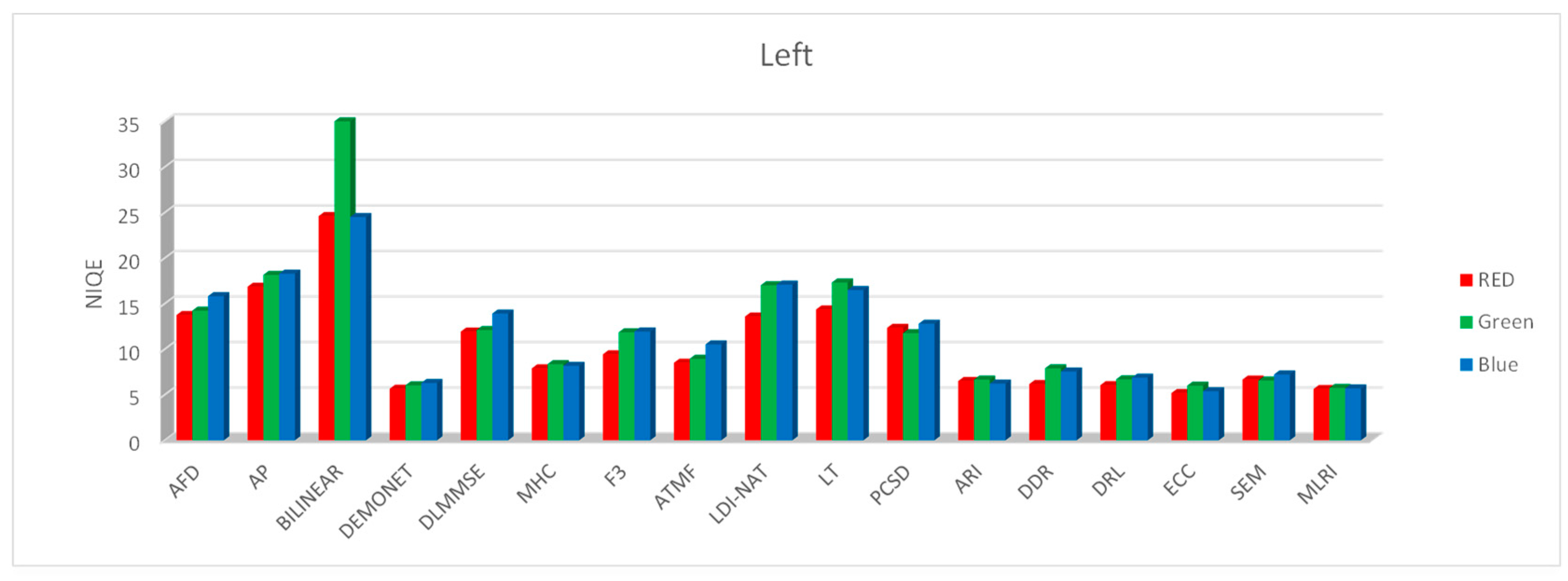
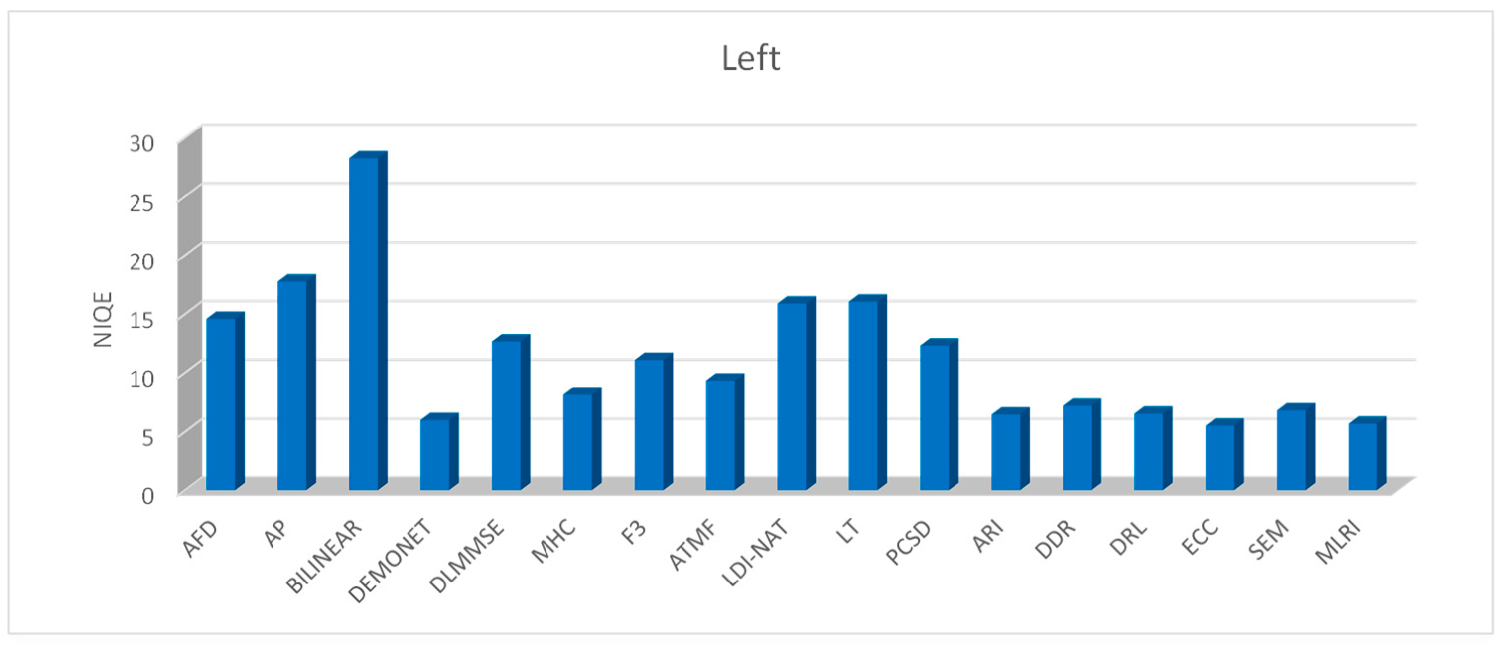
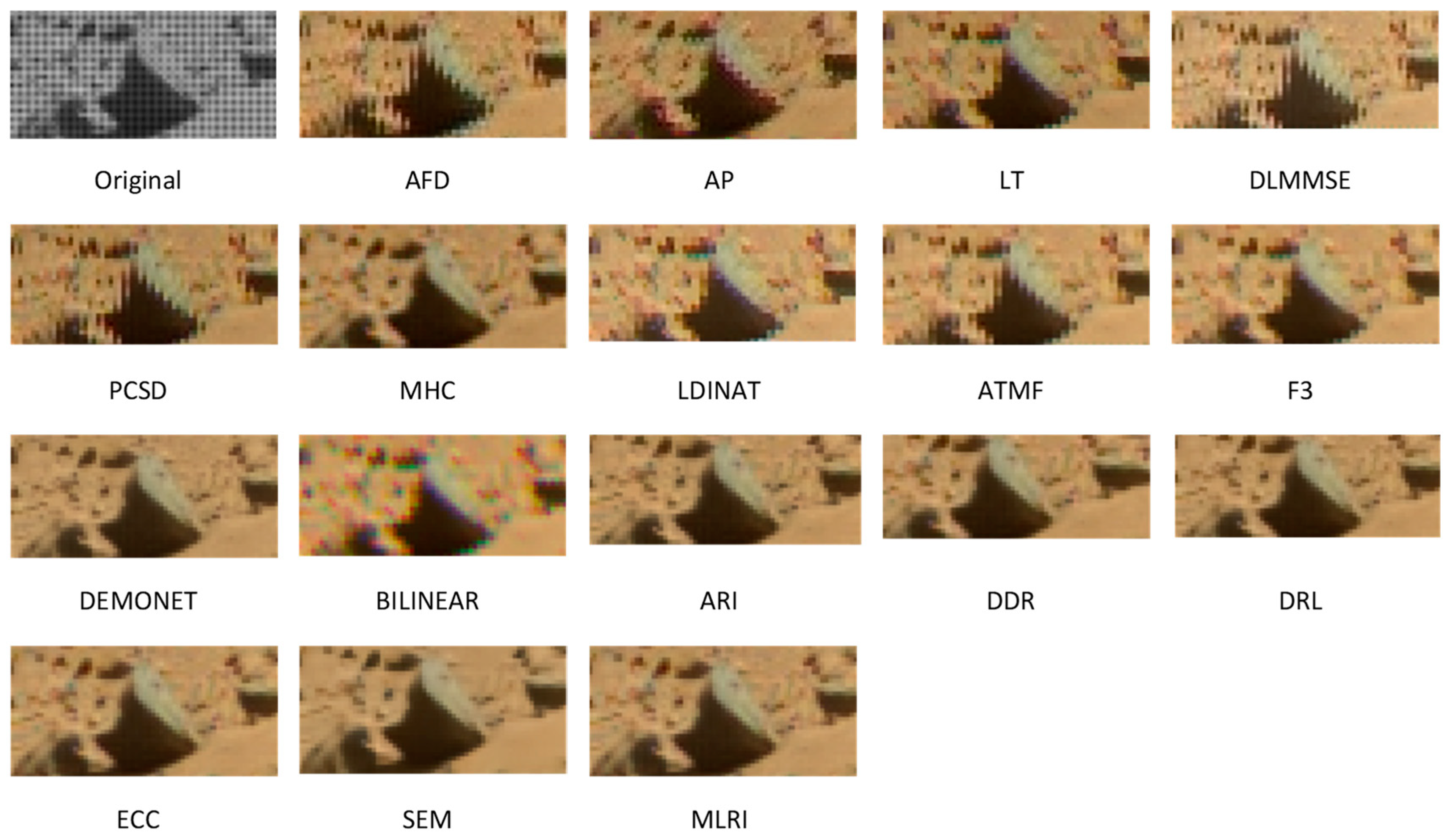
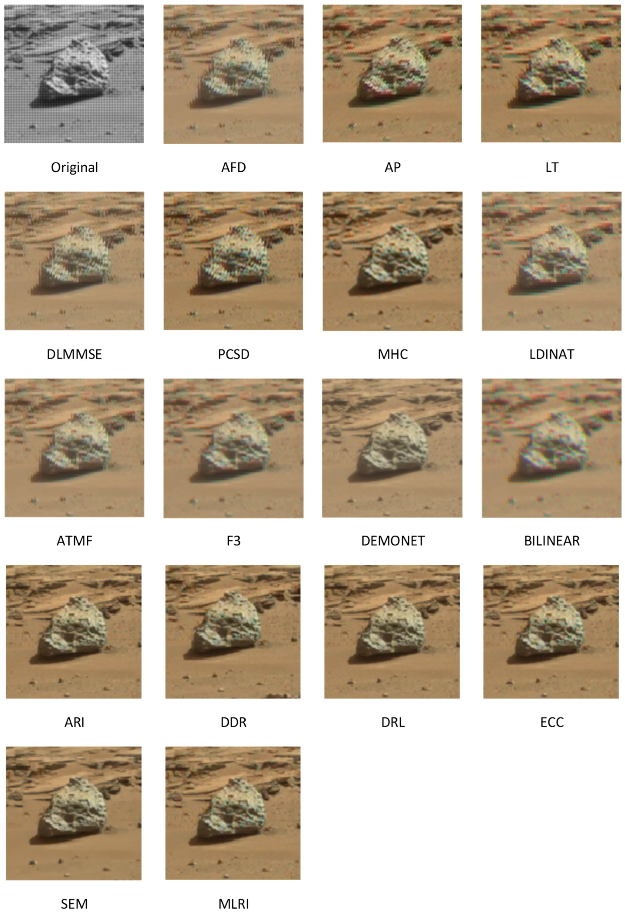
3.2. Left Mastcam Image Demosaicing Results
- The MHC method, which was developed in 2004 and is currently being used by NASA, is mediocre in terms of average scores. Seven algorithms have better results.
- The non-deep learning based method known as ECC achieved the best performance for left images in red and blue bands. However, MLRI has good performance in the green band.
- From Table 4, DEMONET performed the best amongst the deep learning algorithms. Its averaged score (5.98) is close to that of ECC (5.51).
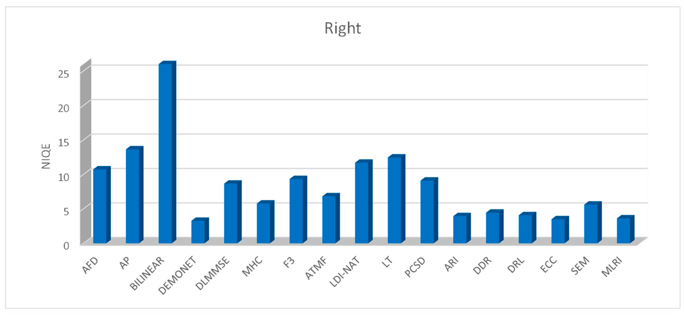
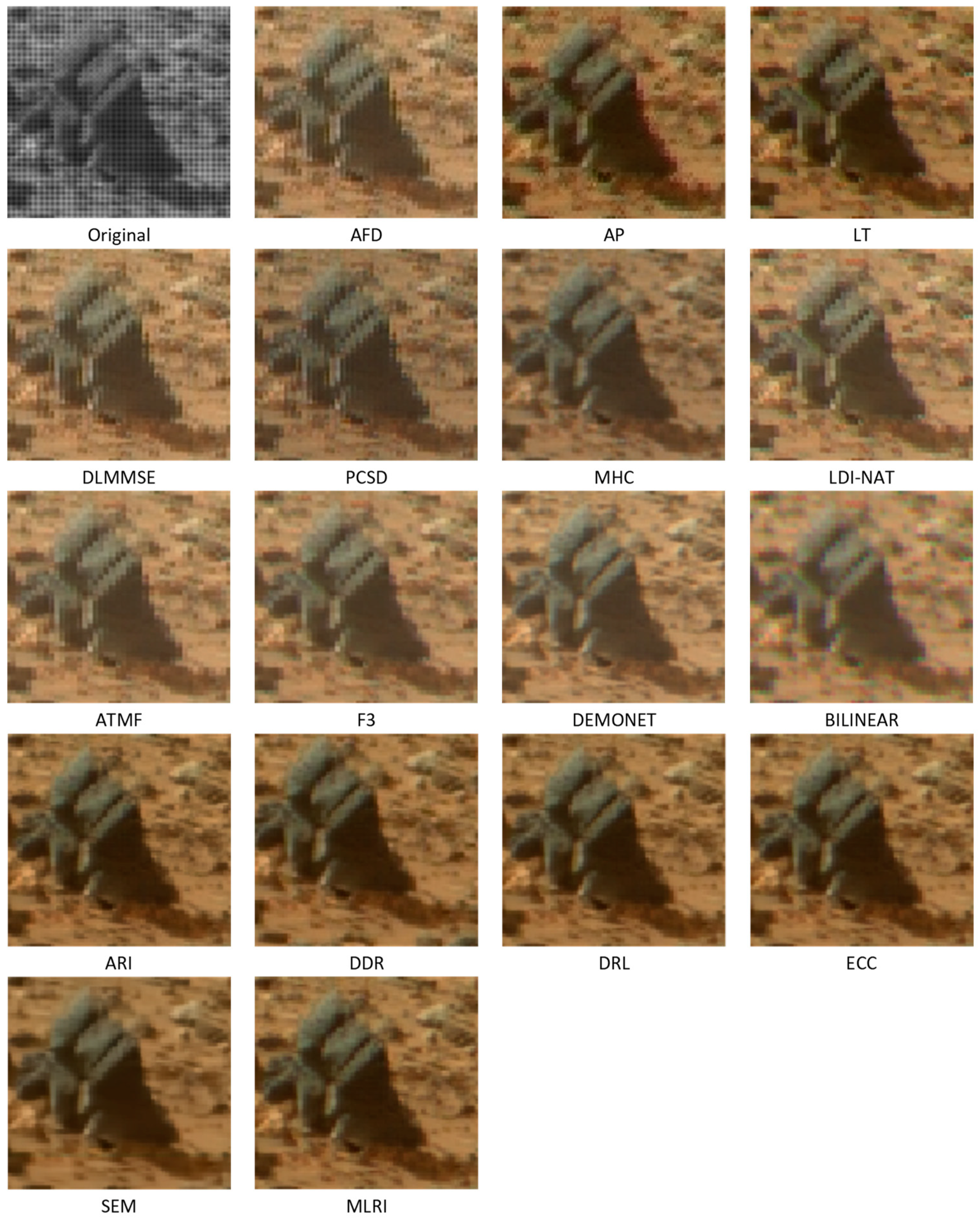
3.3. Right Mastcam Image Demosaicing Results
- In general, the NIQE scores are lower in the right images than those in the left images. This is because the right images have three times higher resolution than those of the left. As a result, neighboring pixels have better correlation, and hence it is easier to demosaic in right images.
- In right images, DEMONET has the best performance in all images.
- MHC is again the mediocre algorithm, as there are seven other algorithms that performed better.
- Among the three deep learning methods (SEM, DEMONET, DRL), DEMONET performed the best.
- There are several non-deep learning based algorithms (ECC, ARI, MLRI) that performed better than two of the deep learning based methods (SEM and DRL).
- Among the non-deep learning based algorithms, ECC is the best performing one.
4. Conclusions
Author Contributions
Funding
Conflicts of Interest
References
- Bell, J.F., III; Godber, A.; McNair, S.; Caplinger, M.A.; Maki, J.N.; Lemmon, M.T.; Van Beek, J.; Malin, M.C.; Wellington, D.; Kinch, K.; et al. The Mars Science Laboratory Curiosity rover Mastcam instruments: Preflight and in-flight calibration, validation, and data archiving. Earth Space Sci. 2017, 4, 396–452. [Google Scholar] [CrossRef]
- Ayhan, B.; Kwan, C.; Vance, S. On the Use of a Linear Spectral Unmixing Technique for Concentration Estimation of APXS Spectrum. J. Multidiscip. Eng. Sci. Technol. 2015, 2, 2469–2474. [Google Scholar]
- Wang, W.; Li, S.; Qi, H.; Ayhan, B.; Kwan, C.; Vance, S. Revisiting the Preprocessing Procedures for Elemental Concentration Estimation based on CHEMCAM LIBS on MARS Rover. In Proceedings of the 6th Workshop on Hyperspectral Image and Signal Processing: Evolution in Remote Sensing (WHISPERS), Lausanne, Switzerland, 24–27 June 2014. [Google Scholar]
- Wang, W.; Ayhan, B.; Kwan, C.; Qi, H.; Vance, S. A Novel and Effective Multivariate Method for Compositional Analysis using Laser Induced Breakdown Spectroscopy. In Proceedings of the 35th International Symposium on Remote Sensing of Environment, Beijing, China, 22–26 April 2013. [Google Scholar]
- Dao, M.; Kwan, C.; Ayhan, B.; Bell, J.F., III. Enhancing Mastcam Images for Mars Rover Mission. In Proceedings of the 14th International Symposium on Neural Networks, Hokkaido, Japan, 21–26 June 2017; pp. 197–206. [Google Scholar]
- Ayhan, B.; Dao, M.; Kwan, C.; Chen, H.-M.; Bell III, J.F.; Kidd, R. A Novel Utilization of Image Registration Techniques to Process Mastcam Images in Mars Rover with Applications to Image Fusion, Pixel Clustering, and Anomaly Detection. IEEE J. Sel. Top. Appl. Earth Obs. Remote. Sens. 2017, 10, 4553–4564. [Google Scholar] [CrossRef]
- Kwan, C.; Budavari, B.; Dao, M.; Ayhan, B.; Bell, J.F., III. Pansharpening of Mastcam images. In Proceedings of the IEEE International Geoscience and Remote Sensing Symposium, Fort Worth, TX, USA, 23–28 July 2017; pp. 5117–5120. [Google Scholar]
- Kwan, C.; Dao, M.; Chou, B.; Kwan, L.M.; Ayhan, B. Mastcam Image Enhancement Using Estimated Point Spread Functions. In Proceedings of the IEEE 8th Annual Ubiquitous Computing, Electronics and Mobile Communication Conference (UEMCON), New York City, NY, USA, 19–21 October 2017. [Google Scholar]
- Malin, M.C.; Ravine, M.A.; Caplinger, M.A.; Ghaemi, F.T.; Schaffner, J.A.; Maki, J.N.; Bell, J.F., III; Cameron, J.F.; Dietrich, W.E.; Edgett, K.S.; et al. The Mars Science Laboratory (MSL) mast cameras and descent imager: I. Investigation and instrument descriptions. Earth Space Sci. 2017, 4, 2. [Google Scholar] [CrossRef] [PubMed]
- Qu, Y.; Guo, R.; Wang, W.; Qi, H.; Ayhan, B.; Kwan, C.; Vance, S. Anomaly Detection in Hyperspectral Images Through Spectral Unmixing and Low Rank Decomposition. In Proceedings of the IEEE International Geoscience and Remote Sensing Symposium (IGARSS), Beijing, China, 10–15 July 2016. [Google Scholar]
- Bayer, B.E. Color Imaging Array. U.S. Patent 3,971,065, 20 July 1976. [Google Scholar]
- Li, X.; Gunturk, B.; Zhang, L. Image demosaicing: A systematic survey. In Proceedings of the SPIE Visual Communications and Image Processing, San Jose, CA, USA, 27–31 January 2008; p. 6822. [Google Scholar]
- Losson, O.; Macaire, L.; Yang, Y. Comparison of color demosaicing methods. Adv. Imaging Electron. Phys. 2010, 162, 173–265. [Google Scholar]
- Kwan, C.; Chou, B.; Kwan, L.-Y.M.; Budavari, B. Debayering RGBW color filter arrays: A pansharpening approach. In Proceedings of the IEEE 8th Annual Ubiquitous Computing, Electronics and Mobile Communication Conference (UEMCON), New York, NY, USA, 19–21 October 2017; pp. 94–100. [Google Scholar]
- Kwan, C.; Chou, B. Further Improvement of Debayering Performance of RGBW Color Filter Arrays Using Deep Learning and Pansharpening Techniques. J. Imaging 2019. submitted. [Google Scholar]
- Zhang, L.; Wu, X.; Buades, A.; Li, X. Color demosaicking by local directional interpolation and nonlocal adaptive thresholding. J. Electron. Imaging 2011, 20. [Google Scholar]
- Malvar, H.S.; He, L.-W.; Cutler, R. High-quality linear interpolation for demosaciking of color images. In Proceedings of the IEEE International Conference on Acoustics, Speech, and Signal Processing, Montreal, QC, Canada, 17–21 May 2004; pp. 485–488. [Google Scholar]
- Zhang, L.; Wu, X. Color demosaicking via directional linear minimum mean square-error estimation. IEEE Trans. Image Process. 2005, 14, 2167–2178. [Google Scholar] [CrossRef] [PubMed]
- Gharbi, M.; Chaurasia, G.; Paris, S.; Durand, F. Deep joint demosaicking and denoising. ACM Trans. Graph. 2016, 35, 191. [Google Scholar] [CrossRef]
- Tan, R.; Zhang, K.; Zuo, W.; Zhang, L. Color image demosaicking via deep residual learning. In Proceedings of the IEEE International Conference on Multimedia and Expo (ICME), Hong Kong, China, 14–17 July 2017; pp. 793–798. [Google Scholar]
- Klatzer, T.; Hammernik, K.; Knobelreiter, P.; Pock, T. Learning joint demosaicing and denoising based on sequential energy minimization. In Proceedings of the IEEE International Conference on Computational Photography (ICCP), Evanston, IL, USA, 13–15 May 2016; pp. 1–11. [Google Scholar]
- Kwan, C.; Chou, B.; Kwan, L.M.; Larkin, J.; Ayhan, B.; Bell, J.F., III; Kerner, H. Demosaicking enhancement using pixel-level fusion. Signal. Image Video Process. 2018, 12, 749–756. [Google Scholar] [CrossRef]
- Bednar, J.; Watt, T. Alpha-trimmed means and their relationship to median filters. IEEE Trans. Acoust. Speech Signal. Process. 1984, 32, 145–153. [Google Scholar] [CrossRef]
- Lu, W.; Tan, Y.-P. Color filter array demosaicking: New method and performance measures. IEEE Trans. Image Process. 2003, 12, 1194–1210. [Google Scholar] [PubMed]
- Dubois, E. Frequency-domain methods for demosaicking of Bayer-sampled color images. IEEE Signal. Proc. Lett. 2005, 12, 847–850. [Google Scholar] [CrossRef]
- Gunturk, B.K.; Altunbasak, Y.; Mersereau, R.M. Color plane interpolation using alternating projections. IEEE Trans. Image Process. 2002, 11, 997–1013. [Google Scholar] [CrossRef] [PubMed]
- Wu, X.; Zhang, N. Primary-consistent soft-decision color demosaicking for digital cameras. IEEE Trans. Image Process. 2004, 13, 1263–1274. [Google Scholar] [CrossRef]
- Jaiswal, S.P.; Au, O.C.; Jakhetiya, V.; Yuan, Y.; Yang, H. Exploitation of inter-color correlation for color image demosaicking. In Proceedings of the 2014 IEEE International Conference on Image Processing (ICIP), Paris, France, 27–30 October 2014; pp. 1812–1816. [Google Scholar]
- Monno, Y.; Kiku, D.; Tanaka, M.; Okutomi, M. Adaptive Residual Interpolation for Color and Multispectral Image Demosaicking. Sensors 2017, 17, 2787. [Google Scholar] [CrossRef] [PubMed]
- Wu, J.; Timofte, R.; Van Gool, L. Demosaicing based on directional difference regression and efficient regression priors. IEEE Trans. Image Process. 2016, 25, 3862–3874. [Google Scholar] [CrossRef] [PubMed]
- Kiku, D.; Monno, Y.; Tanaka, M.; Okutomi, M. Beyond color difference: Residual interpolation for color image demosaicking. IEEE Trans. Image Process. 2016, 25, 1288–1300. [Google Scholar] [CrossRef] [PubMed]
- Mittal, A.; Soundararajan, R.; Bovik, A.C. Making a completely blind image quality analyzer. IEEE Signal. Process. Lett. 2013, 22, 209–212. [Google Scholar] [CrossRef]
- Kwan, C.; Budavari, B.; Bovik, A.; Marchisio, G. Blind quality assessment of fused WorldView-3 images by using the combinations of pansharpening and hypersharpening paradigms. IEEE Geosci. Remote Sens. Lett. 2017, 14, 1835–1839. [Google Scholar] [CrossRef]
- Zhang, X.; Wandell, B.A. A spatial extension of cielab for digital color image reproduction. J. Soc. Inf. Disp. 1997, 5, 61–63. [Google Scholar] [CrossRef]


| 1 | 2 | 3 | 4 | 5 | 6 | 7 | 8 | 9 | 10 | 11 | 12 | 13 | 14 | 15 | 16 | Average Score | |
|---|---|---|---|---|---|---|---|---|---|---|---|---|---|---|---|---|---|
| AFD | 12.6157 | 12.3485 | 12.1242 | 13.3303 | 13.2126 | 13.5321 | 14.7531 | 15.1553 | 18.6010 | 10.9798 | 10.1270 | 9.9302 | 9.9043 | 17.9503 | 15.2261 | 20.0289 | 13.7387 |
| AP | 18.2010 | 18.0048 | 19.4864 | 17.5491 | 15.8528 | 16.5753 | 18.1528 | 16.4546 | 16.8276 | 13.0121 | 11.9930 | 13.4964 | 14.7574 | 17.2369 | 18.4499 | 23.5608 | 16.8507 |
| BILINEAR | 24.3861 | 22.7447 | 24.9261 | 21.5132 | 27.4676 | 23.5540 | 20.5943 | 32.9269 | 36.3999 | 19.8422 | 19.0712 | 18.7308 | 22.4578 | 27.4981 | 29.3003 | 22.2328 | 24.6029 |
| DEMONET | 6.3888 | 6.2854 | 6.2401 | 4.9996 | 6.4177 | 5.2067 | 8.1258 | 7.0335 | 7.5684 | 2.3706 | 2.5799 | 2.7853 | 3.1433 | 6.0430 | 5.4516 | 9.7968 | 5.6523 |
| DLMMSE | 9.4969 | 9.8020 | 8.9876 | 9.9526 | 10.6303 | 9.5661 | 11.9049 | 15.9125 | 19.0670 | 9.2243 | 8.8326 | 8.5922 | 8.3645 | 17.2780 | 16.6125 | 16.5366 | 11.9225 |
| MHC | 8.8028 | 8.4880 | 8.4972 | 6.5740 | 7.7228 | 6.8218 | 8.0547 | 10.2574 | 9.1416 | 5.8709 | 6.0534 | 5.7102 | 6.4907 | 8.9529 | 8.4660 | 10.3326 | 7.8898 |
| F3 | 9.9487 | 9.4586 | 9.8147 | 8.3603 | 9.7182 | 8.0768 | 10.3871 | 12.0146 | 10.6184 | 7.5044 | 7.6903 | 7.8860 | 7.9320 | 10.0270 | 9.5595 | 11.9133 | 9.4319 |
| ATMF | 7.5744 | 7.5672 | 7.4194 | 6.6482 | 8.0566 | 7.0440 | 9.2500 | 12.5748 | 12.2874 | 6.5111 | 6.8925 | 6.4804 | 6.9250 | 10.6036 | 10.0881 | 10.1432 | 8.5041 |
| LDI-NAT | 15.2696 | 13.8418 | 14.1918 | 13.0392 | 16.0519 | 11.4435 | 14.1575 | 18.6315 | 13.4045 | 9.9377 | 10.4555 | 10.7327 | 10.2377 | 13.7882 | 14.1493 | 17.9184 | 13.5782 |
| LT | 16.2990 | 16.1489 | 14.7652 | 14.5088 | 15.4279 | 12.9803 | 16.4634 | 16.2705 | 15.0118 | 10.6679 | 10.5675 | 10.7996 | 11.0427 | 14.2605 | 14.5101 | 19.9576 | 14.3551 |
| PCSD | 10.6626 | 9.5610 | 10.5258 | 11.1919 | 11.5831 | 11.3474 | 13.2739 | 15.1180 | 16.6131 | 10.3915 | 10.0033 | 9.4892 | 10.4619 | 16.1212 | 15.0266 | 16.0245 | 12.3372 |
| ARI | 7.8307 | 7.7902 | 7.6098 | 6.4998 | 7.1966 | 5.5262 | 8.8072 | 7.5124 | 8.4496 | 2.7482 | 3.0267 | 3.1441 | 3.7501 | 6.7718 | 6.8560 | 10.4665 | 6.4991 |
| DDR | 7.3324 | 6.5304 | 7.4349 | 5.4152 | 7.4710 | 5.3931 | 7.4163 | 6.7847 | 8.1394 | 2.8828 | 3.3034 | 3.5171 | 3.8357 | 6.0895 | 6.0212 | 11.0807 | 6.1655 |
| DRL | 6.6865 | 6.4329 | 6.6929 | 5.4711 | 6.9394 | 6.1882 | 8.1536 | 7.3102 | 7.3954 | 2.5361 | 2.9083 | 3.1997 | 3.4499 | 6.2047 | 6.3336 | 10.7963 | 6.0437 |
| ECC | 6.1652 | 5.9417 | 5.7833 | 4.4966 | 5.8008 | 4.6530 | 7.1787 | 5.7831 | 8.0893 | 2.0770 | 2.4203 | 2.7926 | 2.8901 | 5.0870 | 4.8711 | 8.8361 | 5.1791 |
| SEM | 8.2160 | 7.3065 | 6.8650 | 6.0870 | 6.4451 | 6.4901 | 6.2254 | 6.5468 | 7.4197 | 4.2544 | 4.1907 | 4.6557 | 4.6339 | 6.3160 | 6.9174 | 13.9538 | 6.6577 |
| MLRI | 6.2695 | 6.1110 | 6.3910 | 5.0862 | 6.4207 | 5.0127 | 8.0620 | 6.1697 | 8.5279 | 2.3714 | 2.6752 | 2.8781 | 3.2375 | 5.6602 | 5.5172 | 9.5773 | 5.6230 |
| 1 | 2 | 3 | 4 | 5 | 6 | 7 | 8 | 9 | 10 | 11 | 12 | 13 | 14 | 15 | 16 | Average Score | |
|---|---|---|---|---|---|---|---|---|---|---|---|---|---|---|---|---|---|
| AFD | 12.6703 | 12.6311 | 12.3865 | 13.8310 | 14.3111 | 12.9213 | 18.3620 | 16.2041 | 19.5074 | 11.5416 | 10.3887 | 10.2301 | 10.1888 | 18.5937 | 15.9739 | 17.7493 | 14.2182 |
| AP | 20.1798 | 20.9515 | 21.5002 | 19.1573 | 19.5768 | 17.2300 | 18.3290 | 16.6963 | 17.4608 | 13.0597 | 12.6967 | 14.2266 | 14.9722 | 18.0224 | 19.4218 | 26.8274 | 18.1443 |
| BILINEAR | 40.7608 | 39.2980 | 41.1265 | 41.9653 | 45.0438 | 34.1691 | 31.3486 | 41.9754 | 35.3423 | 29.9190 | 27.3598 | 25.3460 | 32.7174 | 37.4109 | 37.1828 | 29.1994 | 35.6353 |
| DEMONET | 7.0640 | 6.9449 | 6.6178 | 5.5862 | 6.8468 | 5.3198 | 9.3102 | 7.2925 | 7.4448 | 2.5248 | 2.8198 | 3.1476 | 3.2791 | 6.3934 | 5.8190 | 9.9502 | 6.0226 |
| DLMMSE | 9.5654 | 10.0626 | 9.2360 | 9.9096 | 12.2185 | 9.2016 | 14.1905 | 16.9864 | 19.5058 | 9.2222 | 8.6287 | 8.3050 | 8.0422 | 17.2357 | 15.9294 | 15.1912 | 12.0894 |
| MHC | 11.0402 | 10.1916 | 9.6517 | 7.3656 | 9.3626 | 6.9627 | 9.1531 | 9.2700 | 9.3979 | 5.3081 | 5.7778 | 5.8543 | 6.2014 | 7.9290 | 8.0201 | 12.1286 | 8.3509 |
| F3 | 13.7498 | 12.3342 | 12.8677 | 11.6409 | 12.3959 | 10.2167 | 13.8089 | 15.8334 | 12.2554 | 9.1715 | 9.0990 | 9.3589 | 10.1732 | 11.6633 | 11.2368 | 13.6424 | 11.8405 |
| ATMF | 8.5114 | 8.4356 | 7.8041 | 7.1378 | 9.8430 | 7.3690 | 10.7015 | 13.0503 | 12.5598 | 6.6034 | 6.8257 | 6.7711 | 6.9102 | 10.2502 | 9.7555 | 10.4899 | 8.9387 |
| LDI-NAT | 20.1918 | 19.6658 | 18.8845 | 17.4088 | 20.7436 | 15.1318 | 18.3224 | 23.7702 | 15.2608 | 12.3106 | 12.2848 | 12.0722 | 12.5477 | 16.1586 | 17.3386 | 20.0246 | 17.0073 |
| LT | 22.7623 | 22.6173 | 19.8021 | 17.5254 | 18.0994 | 15.9179 | 18.1351 | 20.6919 | 16.1980 | 11.9799 | 12.3960 | 12.9244 | 13.2472 | 16.6548 | 17.3158 | 20.7084 | 17.3110 |
| PCSD | 9.0432 | 8.8867 | 8.8222 | 9.6742 | 11.5718 | 10.1917 | 13.6950 | 14.8333 | 18.6161 | 10.1609 | 9.2967 | 8.9027 | 9.2410 | 16.6378 | 14.1500 | 14.2234 | 11.7467 |
| ARI | 7.6321 | 7.7683 | 6.9852 | 6.1566 | 7.7425 | 5.7470 | 10.4436 | 7.2718 | 7.6983 | 2.9622 | 3.1619 | 3.4485 | 3.7585 | 6.5774 | 6.8704 | 12.1917 | 6.6510 |
| DDR | 10.4109 | 8.9291 | 9.4875 | 7.5457 | 9.3295 | 6.9483 | 9.7873 | 8.2933 | 8.1583 | 3.8448 | 4.3701 | 4.7332 | 5.0439 | 7.1323 | 7.0400 | 15.1946 | 7.8905 |
| DRL | 7.9368 | 7.4567 | 7.3435 | 6.3023 | 7.9834 | 5.7111 | 9.0479 | 7.7064 | 7.1232 | 2.8032 | 3.0707 | 3.4920 | 3.6821 | 6.6151 | 6.5001 | 14.0444 | 6.6762 |
| ECC | 7.7006 | 6.8815 | 6.2364 | 5.0943 | 6.8910 | 5.6091 | 8.5025 | 5.7033 | 7.9690 | 2.6572 | 2.8357 | 3.2388 | 3.2777 | 5.2952 | 5.2841 | 12.5825 | 5.9849 |
| SEM | 7.7693 | 6.8767 | 6.5279 | 6.1042 | 6.3507 | 6.2772 | 6.1881 | 6.7558 | 7.0327 | 4.3574 | 4.1155 | 4.7189 | 4.7257 | 6.5027 | 6.8619 | 13.6116 | 6.5485 |
| MLRI | 6.3992 | 6.6364 | 5.7877 | 4.8804 | 6.2366 | 5.1377 | 8.4950 | 5.9310 | 8.0001 | 2.7079 | 2.6687 | 2.9962 | 3.2730 | 5.4421 | 5.5927 | 11.6218 | 5.7379 |
| 1 | 2 | 3 | 4 | 5 | 6 | 7 | 8 | 9 | 10 | 11 | 12 | 13 | 14 | 15 | 16 | Average Score | |
|---|---|---|---|---|---|---|---|---|---|---|---|---|---|---|---|---|---|
| AFD | 14.5864 | 13.9231 | 14.0585 | 15.3444 | 18.5497 | 15.5466 | 18.7568 | 17.3559 | 19.8981 | 13.6431 | 12.4304 | 12.0565 | 12.4879 | 18.7383 | 16.9312 | 18.7096 | 15.8135 |
| AP | 19.2670 | 19.9871 | 21.3419 | 19.3088 | 19.3347 | 17.5124 | 19.2153 | 17.6247 | 18.2528 | 13.3385 | 13.2465 | 14.5793 | 15.2625 | 19.7025 | 20.2802 | 24.2563 | 18.2819 |
| BILINEAR | 23.8308 | 20.8149 | 24.6371 | 21.6647 | 24.1133 | 19.8129 | 20.3025 | 40.5546 | 35.3253 | 18.3366 | 20.0293 | 18.0607 | 19.3285 | 32.7385 | 31.7767 | 20.6639 | 24.4994 |
| DEMONET | 7.2567 | 6.6519 | 6.6649 | 5.9576 | 7.4158 | 5.6743 | 8.8996 | 7.8555 | 7.5587 | 3.1536 | 3.1706 | 3.4218 | 3.6073 | 7.1296 | 6.2235 | 9.9246 | 6.2854 |
| DLMMSE | 10.9357 | 10.7937 | 10.0314 | 11.7147 | 15.2816 | 11.0944 | 18.2778 | 20.5719 | 20.2985 | 11.2449 | 10.0133 | 9.9414 | 9.3345 | 20.4301 | 17.6373 | 14.8350 | 13.9023 |
| MHC | 8.7606 | 8.0585 | 8.0009 | 6.8194 | 10.9248 | 7.0562 | 11.1300 | 10.7483 | 9.0195 | 5.8184 | 5.9876 | 5.6556 | 5.6390 | 8.3535 | 8.1691 | 10.5054 | 8.1654 |
| F3 | 13.7223 | 12.4385 | 13.0771 | 10.6563 | 15.8835 | 9.5145 | 14.1971 | 16.4787 | 11.8411 | 8.8933 | 9.0591 | 9.0519 | 9.5685 | 11.7786 | 12.5635 | 12.2013 | 11.9328 |
| ATMF | 9.3318 | 9.2339 | 9.0547 | 8.7640 | 12.2586 | 8.2443 | 13.3870 | 14.7837 | 14.6702 | 8.4970 | 8.0584 | 8.0154 | 7.6959 | 12.8762 | 12.4575 | 10.9242 | 10.5158 |
| LDI-NAT | 19.5850 | 18.1983 | 19.8057 | 16.8455 | 21.4798 | 13.4044 | 18.7152 | 24.5553 | 15.6810 | 12.0656 | 12.5384 | 13.3025 | 12.3000 | 17.8838 | 18.9332 | 18.0008 | 17.0809 |
| LT | 18.3088 | 19.1614 | 18.4159 | 16.9973 | 18.7274 | 14.4921 | 16.7091 | 18.8571 | 15.7428 | 12.1769 | 12.2158 | 13.1784 | 12.7667 | 19.0153 | 18.0692 | 18.9609 | 16.4872 |
| PCSD | 9.5105 | 9.6314 | 9.6460 | 10.8682 | 13.5822 | 10.7944 | 14.1071 | 16.8850 | 19.9891 | 11.2238 | 9.7191 | 9.3630 | 9.6811 | 18.1334 | 16.8122 | 14.6453 | 12.7870 |
| ARI | 7.5236 | 7.5462 | 6.7914 | 6.1973 | 6.5027 | 5.2371 | 8.9051 | 7.1753 | 7.4235 | 2.8278 | 2.9863 | 3.2339 | 3.6053 | 6.1213 | 6.1758 | 11.1646 | 6.2136 |
| DDR | 8.8834 | 8.5042 | 8.5348 | 7.1919 | 8.8674 | 7.0034 | 9.5343 | 8.6183 | 8.1761 | 4.0088 | 4.4167 | 4.7057 | 4.9941 | 7.5178 | 7.5042 | 12.1168 | 7.5361 |
| DRL | 7.5994 | 7.7727 | 7.2424 | 6.2941 | 8.5154 | 6.1257 | 10.1854 | 8.4451 | 8.0437 | 3.4442 | 3.5534 | 3.8158 | 4.1140 | 7.3694 | 7.1362 | 10.2393 | 6.8685 |
| ECC | 6.4315 | 6.1222 | 5.7949 | 5.1305 | 5.9310 | 4.9685 | 7.5694 | 6.1103 | 7.2993 | 2.4650 | 2.6389 | 2.9609 | 3.0864 | 5.1252 | 5.1081 | 9.2109 | 5.3721 |
| SEM | 8.8906 | 7.8784 | 7.2367 | 6.6777 | 7.2827 | 6.8169 | 6.7955 | 7.3035 | 7.0705 | 4.9536 | 4.8367 | 5.4966 | 5.3667 | 6.9520 | 7.4696 | 14.4549 | 7.2177 |
| MLRI | 6.7813 | 6.5032 | 6.1632 | 5.2871 | 6.4288 | 5.3377 | 8.1457 | 6.5769 | 7.5407 | 2.6612 | 2.8198 | 3.0884 | 3.2593 | 5.4085 | 5.5196 | 9.3803 | 5.6814 |
| 1 | 2 | 3 | 4 | 5 | 6 | 7 | 8 | 9 | 10 | 11 | 12 | 13 | 14 | 15 | 16 | Average Score | |
|---|---|---|---|---|---|---|---|---|---|---|---|---|---|---|---|---|---|
| AFD | 13.2908 | 12.9676 | 12.8564 | 14.1686 | 15.3578 | 14.0000 | 17.2906 | 16.2384 | 19.3355 | 12.0549 | 10.9820 | 10.7389 | 10.8603 | 18.4274 | 16.0437 | 18.8293 | 14.5901 |
| AP | 19.2159 | 19.6478 | 20.7761 | 18.6718 | 18.2548 | 17.1059 | 18.5657 | 16.9252 | 17.5137 | 13.1368 | 12.6454 | 14.1008 | 14.9974 | 18.3206 | 19.3840 | 24.8815 | 17.7590 |
| BILINEAR | 29.6592 | 27.6192 | 30.2299 | 28.3811 | 32.2082 | 25.8453 | 24.0818 | 38.4856 | 35.6892 | 22.6992 | 22.1534 | 20.7125 | 24.8346 | 32.5492 | 32.7533 | 24.0321 | 28.2459 |
| DEMONET | 6.9032 | 6.6274 | 6.5076 | 5.5145 | 6.8934 | 5.4003 | 8.7785 | 7.3938 | 7.5240 | 2.6830 | 2.8568 | 3.1182 | 3.3432 | 6.5220 | 5.8313 | 9.8905 | 5.9867 |
| DLMMSE | 9.9994 | 10.2194 | 9.4183 | 10.5256 | 12.7101 | 9.9540 | 14.7911 | 17.8236 | 19.6238 | 9.8971 | 9.1582 | 8.9462 | 8.5804 | 18.3146 | 16.7264 | 15.5209 | 12.6381 |
| MHC | 9.5345 | 8.9127 | 8.7166 | 6.9196 | 9.3367 | 6.9469 | 9.4459 | 10.0919 | 9.1864 | 5.6658 | 5.9396 | 5.7400 | 6.1104 | 8.4118 | 8.2184 | 10.9889 | 8.1354 |
| F3 | 12.4736 | 11.4104 | 11.9199 | 10.2192 | 12.6659 | 9.2693 | 12.7977 | 14.7756 | 11.5717 | 8.5231 | 8.6161 | 8.7656 | 9.2246 | 11.1563 | 11.1199 | 12.5856 | 11.0684 |
| ATMF | 8.4725 | 8.4122 | 8.0927 | 7.5167 | 10.0527 | 7.5524 | 11.1128 | 13.4696 | 13.1725 | 7.2038 | 7.2589 | 7.0890 | 7.1770 | 11.2433 | 10.7670 | 10.5191 | 9.3195 |
| LDI-NAT | 18.3488 | 17.2353 | 17.6273 | 15.7645 | 19.4251 | 13.3266 | 17.0650 | 22.3190 | 14.7821 | 11.4379 | 11.7596 | 12.0358 | 11.6951 | 15.9435 | 16.8070 | 18.6479 | 15.8888 |
| LT | 19.1234 | 19.3092 | 17.6610 | 16.3438 | 17.4182 | 14.4634 | 17.1025 | 18.6065 | 15.6509 | 11.6083 | 11.7264 | 12.3008 | 12.3522 | 16.6435 | 16.6317 | 19.8757 | 16.0511 |
| PCSD | 9.7388 | 9.3597 | 9.6647 | 10.5781 | 12.2457 | 10.7778 | 13.6920 | 15.6121 | 18.4061 | 10.5921 | 9.6730 | 9.2516 | 9.7947 | 16.9642 | 15.3296 | 14.9644 | 12.2903 |
| ARI | 7.6621 | 7.7016 | 7.1288 | 6.2846 | 7.1473 | 5.5034 | 9.3853 | 7.3199 | 7.8571 | 2.8460 | 3.0583 | 3.2755 | 3.7046 | 6.4901 | 6.6341 | 11.2743 | 6.4546 |
| DDR | 8.8756 | 7.9879 | 8.4857 | 6.7176 | 8.5560 | 6.4483 | 8.9126 | 7.8988 | 8.1580 | 3.5788 | 4.0301 | 4.3187 | 4.6246 | 6.9132 | 6.8551 | 12.7974 | 7.1974 |
| DRL | 7.4076 | 7.2208 | 7.0930 | 6.0225 | 7.8127 | 6.0083 | 9.1290 | 7.8206 | 7.5207 | 2.9279 | 3.1774 | 3.5025 | 3.7487 | 6.7297 | 6.6566 | 11.6933 | 6.5295 |
| ECC | 6.7658 | 6.3151 | 5.9382 | 4.9071 | 6.2076 | 5.0769 | 7.7502 | 5.8655 | 7.7859 | 2.3998 | 2.6317 | 2.9974 | 3.0847 | 5.1692 | 5.0878 | 10.2098 | 5.5120 |
| SEM | 8.2920 | 7.3539 | 6.8765 | 6.2896 | 6.6928 | 6.5281 | 6.4030 | 6.8687 | 7.1743 | 4.5218 | 4.3810 | 4.9571 | 4.9088 | 6.5902 | 7.0829 | 14.0068 | 6.8080 |
| MLRI | 6.4833 | 6.4169 | 6.1140 | 5.0846 | 6.3620 | 5.1627 | 8.2342 | 6.2259 | 8.0229 | 2.5802 | 2.7212 | 2.9876 | 3.2566 | 5.5036 | 5.5432 | 10.1931 | 5.6807 |
| 1 | 2 | 3 | 4 | 5 | 6 | 7 | 8 | 9 | 10 | 11 | 12 | 13 | 14 | 15 | Average Score | |
|---|---|---|---|---|---|---|---|---|---|---|---|---|---|---|---|---|
| AFD | 8.9373 | 8.7759 | 8.4147 | 7.8949 | 9.9891 | 11.7386 | 12.8431 | 11.4313 | 9.5332 | 8.0114 | 7.8637 | 7.4557 | 10.9986 | 9.4828 | 10.4834 | 9.5902 |
| AP | 11.7636 | 12.0465 | 11.5401 | 11.1604 | 12.1845 | 15.8165 | 13.9067 | 13.4301 | 10.4149 | 12.9089 | 12.6933 | 13.0260 | 13.8336 | 12.8938 | 14.1931 | 12.7874 |
| BILINEAR | 28.8126 | 28.7810 | 30.4590 | 28.4978 | 25.9336 | 14.7615 | 19.0792 | 27.5918 | 30.6576 | 17.3245 | 15.8286 | 17.4058 | 18.1779 | 28.7096 | 29.6889 | 24.1140 |
| DEMONET | 2.9675 | 3.0637 | 3.3210 | 3.2762 | 3.3405 | 2.8246 | 2.1394 | 2.4837 | 4.7563 | 2.9169 | 2.8299 | 3.1901 | 5.1096 | 3.4419 | 2.8021 | 3.2309 |
| DLMMSE | 7.8138 | 8.3816 | 7.8904 | 7.4860 | 9.7922 | 9.7494 | 9.5454 | 11.8459 | 8.3049 | 7.3125 | 6.2269 | 6.0346 | 8.1370 | 7.9481 | 11.2107 | 8.5120 |
| MHC | 5.3547 | 5.9482 | 5.4479 | 5.4481 | 7.3170 | 6.3724 | 6.1576 | 7.5658 | 5.6747 | 5.0677 | 4.8282 | 4.3008 | 5.1746 | 6.0824 | 7.6604 | 5.8934 |
| F3 | 8.7640 | 8.7259 | 8.4800 | 7.7582 | 9.5665 | 10.2421 | 10.1394 | 11.7106 | 7.7857 | 8.3091 | 7.4829 | 7.1931 | 7.8775 | 8.0355 | 9.4304 | 8.7667 |
| ATMF | 6.6743 | 6.6595 | 6.4038 | 5.8089 | 7.2439 | 7.0425 | 7.1295 | 9.2204 | 6.8400 | 5.2451 | 4.7606 | 4.7055 | 5.2618 | 5.9143 | 7.8990 | 6.4539 |
| LDI-NAT | 9.2965 | 9.7399 | 9.3430 | 9.5120 | 10.8810 | 12.0612 | 11.2467 | 13.7934 | 8.2312 | 10.3715 | 9.1168 | 9.1195 | 10.6429 | 8.6974 | 10.9420 | 10.1997 |
| LT | 10.6002 | 10.7115 | 10.2027 | 10.3402 | 10.6377 | 12.9606 | 11.8765 | 13.6656 | 8.9471 | 10.3509 | 9.5417 | 9.6351 | 11.1062 | 9.5586 | 12.0835 | 10.8145 |
| PCSD | 8.4732 | 8.1432 | 8.2082 | 8.0098 | 9.3474 | 10.5576 | 10.6419 | 10.9943 | 11.5698 | 7.6042 | 7.0000 | 6.8201 | 8.1520 | 10.0265 | 10.6231 | 9.0781 |
| ARI | 3.8643 | 3.8832 | 3.7584 | 3.6326 | 3.6848 | 3.7225 | 3.4176 | 4.0140 | 4.8334 | 3.6318 | 3.5733 | 3.7651 | 4.8328 | 3.4707 | 3.4006 | 3.8323 |
| DDR | 3.5730 | 3.6052 | 3.4872 | 3.3958 | 3.7071 | 4.2683 | 3.3111 | 3.2884 | 4.4908 | 3.5341 | 3.5813 | 3.8145 | 5.2901 | 3.1349 | 3.6475 | 3.7420 |
| DRL | 4.3763 | 4.6736 | 4.1437 | 4.3016 | 4.4772 | 4.6836 | 3.9870 | 3.6093 | 5.9920 | 4.2541 | 4.1115 | 4.3783 | 5.6772 | 3.9266 | 4.3381 | 4.4620 |
| ECC | 3.3683 | 3.3292 | 3.3833 | 3.4280 | 3.6901 | 3.3630 | 3.1023 | 2.8801 | 5.0862 | 3.1662 | 2.9537 | 3.1822 | 4.1965 | 3.2978 | 3.2007 | 3.4418 |
| SEM | 6.4175 | 6.7539 | 6.2270 | 7.0319 | 6.6929 | 3.9100 | 3.7460 | 5.0608 | 5.7326 | 4.1348 | 4.2521 | 5.4342 | 7.4946 | 5.5833 | 6.2933 | 5.6510 |
| MLRI | 3.3507 | 3.3433 | 3.2649 | 3.1270 | 3.2436 | 3.7696 | 3.2913 | 3.1710 | 4.8223 | 3.4419 | 3.1855 | 3.3245 | 4.2431 | 3.1748 | 2.9723 | 3.4484 |
| 1 | 2 | 3 | 4 | 5 | 6 | 7 | 8 | 9 | 10 | 11 | 12 | 13 | 14 | 15 | Average Score | |
|---|---|---|---|---|---|---|---|---|---|---|---|---|---|---|---|---|
| AFD | 10.2283 | 9.9450 | 10.0469 | 8.9331 | 11.0748 | 12.3874 | 12.5055 | 12.6413 | 9.6722 | 8.8446 | 8.1703 | 7.5573 | 11.4522 | 10.3896 | 12.0499 | 10.3932 |
| AP | 13.2241 | 12.7496 | 12.6944 | 13.2560 | 14.8596 | 16.9524 | 15.3472 | 13.9157 | 12.4708 | 13.9361 | 13.5262 | 13.8971 | 15.2199 | 14.5889 | 13.9971 | 14.0423 |
| BILINEAR | 35.4112 | 33.4531 | 33.5375 | 32.1076 | 32.0812 | 23.6092 | 28.2909 | 38.5868 | 32.8474 | 27.5611 | 19.2977 | 20.2725 | 23.6938 | 33.8324 | 38.2297 | 30.1875 |
| DEMONET | 2.8300 | 2.8854 | 2.9407 | 3.0127 | 3.1893 | 3.0187 | 2.0252 | 2.3617 | 4.0645 | 3.0288 | 2.7233 | 2.8771 | 4.2383 | 3.3213 | 3.0590 | 3.0384 |
| DLMMSE | 7.3204 | 7.5524 | 7.6667 | 7.4579 | 8.8528 | 9.6833 | 9.3913 | 11.3895 | 8.3860 | 7.0783 | 5.9558 | 5.4538 | 7.2602 | 8.1940 | 10.6806 | 8.1549 |
| MHC | 4.7724 | 4.8642 | 4.8707 | 4.8521 | 5.1707 | 6.2827 | 5.2994 | 5.7075 | 5.1135 | 5.2209 | 4.7714 | 4.5538 | 6.7551 | 4.9248 | 5.8384 | 5.2665 |
| F3 | 9.0362 | 9.0262 | 8.9231 | 8.0461 | 10.0338 | 11.1550 | 10.3404 | 12.5021 | 8.3595 | 9.8269 | 8.9642 | 8.0894 | 9.6839 | 8.9083 | 10.5739 | 9.5646 |
| ATMF | 6.2075 | 6.4776 | 6.2349 | 5.7986 | 6.8841 | 7.5712 | 7.2522 | 9.1094 | 6.5474 | 5.9517 | 5.2739 | 5.0625 | 5.9398 | 6.0583 | 7.9680 | 6.5558 |
| LDI-NAT | 12.0319 | 11.0222 | 11.7852 | 11.7070 | 12.9594 | 13.7746 | 13.0479 | 16.4539 | 9.7382 | 13.0068 | 11.5174 | 11.5833 | 13.3256 | 11.8053 | 13.6218 | 12.4920 |
| LT | 12.6544 | 11.7003 | 12.4646 | 12.2405 | 13.8234 | 13.6690 | 13.6470 | 16.7674 | 10.6262 | 15.1693 | 14.2864 | 13.7754 | 14.7637 | 12.5160 | 14.6491 | 13.5168 |
| PCSD | 7.9138 | 7.9461 | 8.3462 | 8.0029 | 8.9711 | 9.9546 | 10.0704 | 11.0980 | 10.9626 | 7.3233 | 6.2532 | 5.9437 | 7.2752 | 9.4385 | 10.3597 | 8.6573 |
| ARI | 3.6773 | 3.6637 | 3.5379 | 3.3950 | 3.5790 | 4.5649 | 3.9592 | 3.7183 | 4.9729 | 4.1258 | 3.9438 | 4.2372 | 5.8258 | 3.4715 | 3.5483 | 4.0147 |
| DDR | 4.6053 | 5.2221 | 4.7598 | 4.5665 | 4.3752 | 5.4972 | 4.0005 | 4.1847 | 5.4951 | 4.8847 | 4.8642 | 5.1785 | 7.2650 | 4.1581 | 4.7003 | 4.9171 |
| DRL | 3.2993 | 3.4929 | 3.3397 | 3.2732 | 3.3959 | 4.2842 | 3.2201 | 2.9978 | 4.5287 | 3.5500 | 3.6291 | 4.1059 | 6.0238 | 3.2160 | 3.3621 | 3.7146 |
| ECC | 3.0159 | 3.0625 | 3.1197 | 3.2723 | 3.2585 | 3.3437 | 2.6735 | 2.6450 | 4.3873 | 3.3267 | 2.9858 | 3.4501 | 5.6797 | 2.8642 | 2.8602 | 3.3297 |
| SEM | 5.5644 | 5.9796 | 5.4204 | 6.4380 | 6.1974 | 3.7708 | 3.5829 | 4.6566 | 5.5745 | 4.2964 | 4.3139 | 5.3388 | 7.3200 | 5.4434 | 5.9784 | 5.3250 |
| MLRI | 3.1872 | 3.1842 | 3.1559 | 3.3401 | 3.3998 | 3.8686 | 3.3537 | 3.1066 | 4.5308 | 3.6670 | 3.4663 | 3.7024 | 5.6801 | 3.2627 | 3.0902 | 3.5997 |
| 1 | 2 | 3 | 4 | 5 | 6 | 7 | 8 | 9 | 10 | 11 | 12 | 13 | 14 | 15 | Average Score | |
|---|---|---|---|---|---|---|---|---|---|---|---|---|---|---|---|---|
| AFD | 12.5477 | 11.9409 | 12.4119 | 9.9442 | 12.8377 | 13.9556 | 14.2960 | 14.9113 | 10.4462 | 10.9007 | 10.0915 | 8.7691 | 13.1742 | 12.4651 | 13.8381 | 12.1687 |
| AP | 13.5296 | 13.2034 | 12.5964 | 12.7902 | 14.7256 | 17.1475 | 15.9003 | 13.3022 | 12.5033 | 14.2503 | 13.1017 | 13.3199 | 14.8402 | 15.2030 | 14.6520 | 14.0710 |
| BILINEAR | 23.8644 | 26.6160 | 27.5043 | 25.1093 | 28.0884 | 16.6282 | 20.4687 | 30.4048 | 27.4614 | 21.8034 | 14.2912 | 16.0282 | 16.4314 | 28.5738 | 32.3832 | 23.7105 |
| DEMONET | 3.6025 | 3.3205 | 3.4325 | 3.3256 | 4.0589 | 3.0237 | 2.4499 | 2.7884 | 4.0108 | 3.3536 | 3.1538 | 3.3053 | 4.6468 | 3.8813 | 4.3289 | 3.5122 |
| DLMMSE | 8.5264 | 8.7596 | 8.6707 | 8.5476 | 9.6663 | 10.5780 | 10.7446 | 12.5295 | 9.6187 | 8.1350 | 6.6076 | 6.2440 | 9.3913 | 9.8253 | 11.5818 | 9.2951 |
| MHC | 6.2451 | 6.3690 | 6.5548 | 6.0205 | 7.2500 | 6.5242 | 6.0671 | 7.5240 | 7.1293 | 5.3466 | 4.5403 | 4.1923 | 5.3854 | 5.7723 | 7.2084 | 6.1419 |
| F3 | 8.3102 | 8.3781 | 8.4115 | 8.2123 | 9.3660 | 11.4006 | 10.7494 | 14.1100 | 8.1449 | 10.0275 | 8.6781 | 8.1412 | 10.1294 | 9.2251 | 11.2337 | 9.6345 |
| ATMF | 7.1593 | 6.9848 | 7.2341 | 6.5064 | 7.7006 | 8.6775 | 8.4664 | 10.6989 | 7.4679 | 6.6607 | 5.5655 | 5.2368 | 6.7328 | 7.2673 | 9.3764 | 7.4490 |
| LDI-NAT | 11.1834 | 10.2198 | 10.1846 | 10.7598 | 12.7046 | 14.1219 | 14.0287 | 16.5706 | 8.7091 | 14.3474 | 12.0921 | 11.7074 | 13.6881 | 12.1656 | 13.3946 | 12.3919 |
| LT | 11.8153 | 11.1057 | 11.2251 | 11.6244 | 13.2907 | 13.9863 | 13.8112 | 16.8207 | 9.9657 | 14.3183 | 12.9410 | 13.0936 | 14.3593 | 12.8745 | 14.0450 | 13.0184 |
| PCSD | 9.2291 | 9.0793 | 9.8087 | 9.0227 | 10.3275 | 10.2666 | 10.6311 | 12.7562 | 10.8984 | 7.7754 | 6.8724 | 6.6299 | 7.9110 | 10.3900 | 11.7432 | 9.5561 |
| ARI | 3.4140 | 3.4395 | 3.2791 | 3.4732 | 3.7545 | 3.8988 | 3.5656 | 3.8133 | 4.9650 | 4.0305 | 4.1304 | 4.2627 | 5.5859 | 3.7664 | 4.0767 | 3.9637 |
| DDR | 4.2288 | 4.5550 | 4.2588 | 4.1113 | 4.3614 | 5.7041 | 4.7395 | 4.3866 | 4.4837 | 4.9152 | 4.5909 | 4.7278 | 6.6523 | 3.8431 | 4.4323 | 4.6660 |
| DRL | 3.6402 | 3.6145 | 3.7252 | 3.5532 | 3.3148 | 5.0437 | 4.0088 | 3.4239 | 5.0221 | 4.4532 | 4.0147 | 4.1556 | 5.4063 | 3.3822 | 3.6686 | 4.0285 |
| ECC | 3.3025 | 3.3867 | 3.2667 | 3.6631 | 3.7915 | 3.6648 | 2.9638 | 3.1258 | 4.7044 | 3.5719 | 3.5386 | 3.7569 | 5.1194 | 3.5656 | 3.7446 | 3.6777 |
| SEM | 6.1757 | 6.4499 | 5.8948 | 6.7091 | 6.8396 | 4.3956 | 4.5851 | 5.2785 | 5.7554 | 4.8414 | 4.6764 | 5.6456 | 7.5500 | 6.0228 | 7.0262 | 5.8564 |
| MLRI | 3.4477 | 3.6087 | 3.3960 | 3.6005 | 3.8101 | 4.0409 | 3.4529 | 3.4557 | 4.4991 | 3.8203 | 3.6343 | 3.8192 | 4.9023 | 3.5789 | 3.8469 | 3.7942 |
| 1 | 2 | 3 | 4 | 5 | 6 | 7 | 8 | 9 | 10 | 11 | 12 | 13 | 14 | 15 | Average Score | |
|---|---|---|---|---|---|---|---|---|---|---|---|---|---|---|---|---|
| AFD | 10.5711 | 10.2206 | 10.2911 | 8.9241 | 11.3005 | 12.6939 | 13.2149 | 12.9947 | 9.8839 | 9.2522 | 8.7085 | 7.9274 | 11.8750 | 10.7792 | 12.1238 | 10.7174 |
| AP | 12.8391 | 12.6665 | 12.2770 | 12.4022 | 13.9232 | 16.6388 | 15.0514 | 13.5493 | 11.7963 | 13.6984 | 13.1071 | 13.4143 | 14.6312 | 14.2286 | 14.2807 | 13.6336 |
| BILINEAR | 29.3628 | 29.6167 | 30.5003 | 28.5716 | 28.7011 | 18.3330 | 22.6129 | 32.1945 | 30.3221 | 22.2297 | 16.4725 | 17.9022 | 19.4344 | 30.3719 | 33.4339 | 26.0040 |
| DEMONET | 3.1333 | 3.0899 | 3.2314 | 3.2048 | 3.5296 | 2.9557 | 2.2048 | 2.5446 | 4.2772 | 3.0998 | 2.9023 | 3.1242 | 4.6649 | 3.5482 | 3.3967 | 3.2605 |
| DLMMSE | 7.8869 | 8.2312 | 8.0759 | 7.8305 | 9.4371 | 10.0036 | 9.8938 | 11.9216 | 8.7699 | 7.5086 | 6.2634 | 5.9108 | 8.2628 | 8.6558 | 11.1577 | 8.6540 |
| MHC | 5.4574 | 5.7271 | 5.6244 | 5.4403 | 6.5792 | 6.3931 | 5.8414 | 6.9325 | 5.9725 | 5.2117 | 4.7133 | 4.3490 | 5.7717 | 5.5932 | 6.9024 | 5.7673 |
| F3 | 8.7034 | 8.7101 | 8.6049 | 8.0055 | 9.6554 | 10.9326 | 10.4097 | 12.7743 | 8.0967 | 9.3878 | 8.3751 | 7.8079 | 9.2303 | 8.7230 | 10.4127 | 9.3220 |
| ATMF | 6.6804 | 6.7073 | 6.6243 | 6.0380 | 7.2762 | 7.7637 | 7.6160 | 9.6762 | 6.9518 | 5.9525 | 5.2000 | 5.0016 | 5.9781 | 6.4133 | 8.4145 | 6.8196 |
| LDI-NAT | 10.8373 | 10.3273 | 10.4376 | 10.6596 | 12.1817 | 13.3192 | 12.7744 | 15.6060 | 8.8929 | 12.5752 | 10.9088 | 10.8034 | 12.5522 | 10.8894 | 12.6528 | 11.6945 |
| LT | 11.6900 | 11.1725 | 11.2975 | 11.4017 | 12.5839 | 13.5386 | 13.1116 | 15.7512 | 9.8464 | 13.2795 | 12.2564 | 12.1680 | 13.4097 | 11.6497 | 13.5925 | 12.4499 |
| PCSD | 8.5387 | 8.3895 | 8.7877 | 8.3452 | 9.5487 | 10.2596 | 10.4478 | 11.6161 | 11.1436 | 7.5676 | 6.7085 | 6.4646 | 7.7794 | 9.9517 | 10.9087 | 9.0972 |
| ARI | 3.6519 | 3.6621 | 3.5252 | 3.5003 | 3.6728 | 4.0621 | 3.6474 | 3.8485 | 4.9238 | 3.9294 | 3.8825 | 4.0883 | 5.4148 | 3.5695 | 3.6752 | 3.9369 |
| DDR | 4.1357 | 4.4608 | 4.1686 | 4.0245 | 4.1479 | 5.1565 | 4.0170 | 3.9532 | 4.8232 | 4.4447 | 4.3454 | 4.5736 | 6.4025 | 3.7120 | 4.2600 | 4.4417 |
| DRL | 3.7719 | 3.9270 | 3.7362 | 3.7093 | 3.7293 | 4.6705 | 3.7386 | 3.3437 | 5.1809 | 4.0857 | 3.9184 | 4.2133 | 5.7024 | 3.5083 | 3.7896 | 4.0684 |
| ECC | 3.2289 | 3.2595 | 3.2566 | 3.4545 | 3.5800 | 3.4572 | 2.9132 | 2.8836 | 4.7260 | 3.3549 | 3.1594 | 3.4630 | 4.9985 | 3.2425 | 3.2685 | 3.4831 |
| SEM | 6.0525 | 6.3945 | 5.8474 | 6.7263 | 6.5767 | 4.0255 | 3.9714 | 4.9986 | 5.6875 | 4.4242 | 4.4142 | 5.4728 | 7.4549 | 5.6832 | 6.4326 | 5.6108 |
| MLRI | 3.3285 | 3.3787 | 3.2723 | 3.3559 | 3.4845 | 3.8930 | 3.3660 | 3.2444 | 4.6174 | 3.6431 | 3.4287 | 3.6154 | 4.9418 | 3.3388 | 3.3031 | 3.6141 |
© 2019 by the authors. Licensee MDPI, Basel, Switzerland. This article is an open access article distributed under the terms and conditions of the Creative Commons Attribution (CC BY) license (http://creativecommons.org/licenses/by/4.0/).
Share and Cite
Kwan, C.; Chou, B.; Bell III, J.F. Comparison of Deep Learning and Conventional Demosaicing Algorithms for Mastcam Images. Electronics 2019, 8, 308. https://doi.org/10.3390/electronics8030308
Kwan C, Chou B, Bell III JF. Comparison of Deep Learning and Conventional Demosaicing Algorithms for Mastcam Images. Electronics. 2019; 8(3):308. https://doi.org/10.3390/electronics8030308
Chicago/Turabian StyleKwan, Chiman, Bryan Chou, and James F. Bell III. 2019. "Comparison of Deep Learning and Conventional Demosaicing Algorithms for Mastcam Images" Electronics 8, no. 3: 308. https://doi.org/10.3390/electronics8030308
APA StyleKwan, C., Chou, B., & Bell III, J. F. (2019). Comparison of Deep Learning and Conventional Demosaicing Algorithms for Mastcam Images. Electronics, 8(3), 308. https://doi.org/10.3390/electronics8030308