Abstract
A relevant task in unmanned aerial vehicles (UAV) flight is path planning in environments. This task must be completed using the least possible computing time. The aim of this article is to combine methodologies to optimise the task in time and offer a complete trajectory. The flight environment will be considered as a adaptive discrete mesh, where grids are created with minimal refinement in the search for collision-free spaces. The proposed path planning algorithm for UAV saves computational time and memory resources compared with classical techniques. With the construction of the discrete meshing, a cost response methodology is applied as a discrete deterministic finite automaton (DDFA). A set of optimal partial responses, calculated recursively, indicates the collision-free spaces in the final path for the UAV flight.
1. Introduction
The world market for unmanned aerial vehicles (UAVs) is expanding rapidly, and there are various forecasts and projections regarding the market for unmanned vehicles. The economic impact of integrating UAVs into the National Airspace System in the United States will grow substantially and reach more than billion between 2015 and 2025 [].
A wide diversity of air missions can be completed by UAVs [,] in various scenarios and including outdoor/indoor and water/ground/air/space environments []. The types of missions include military (missile launching drones, bomb-dropping drones, flying camouflaged drones) and civilian (video-graph/photography, disaster response, environment and climate) [,,,,]. A highly demanded task for UAVs is autonomous navigation (either in static or dynamic environments) that optimises the route and minimises the computational cost. Thus, path planning defines the methodology that an autonomous robot must complete to move from an initial location to a final location, deploying its own resources as sensors, actuators, and strategies, while avoiding obstacles during the trip. Several path planning and obstacle avoidance techniques are being used in unmanned ground vehicles (UGVs), autonomous underwater vehicles (AUVs), and unmanned aerial vehicles (UAVs).
From the traditional robotics point of view, numerous works have been developed in which the path planning and obstacle avoidance algorithms perform searches in continuous or discrete Euclidean [] dimensional movement environments. It is important to mention that LaValle in [] has done significant work on sampling-based path planning algorithms. However, although his analysis is complete from a two-dimensional perspective, planning analysis is not completely addressed. An exhaustive study of the growing work on sampling-based algorithms is presented in []. It must be remembered that the path planning problem is NP-hard; and so environmental dimensional increases and UAV kinematics affect problem complexity.
An in-depth review of the current literature shows several works focus on two-dimensional scenarios [] that limit vehicle behaviour to just a flat surface and consider its height as constant by making a dimensional analysis []. However, in complex unstructured situations (including, for example, forests, urban, or underwater environments) a simple algorithm is insufficient and path planning is needed.
A diversity of methodological paradigms have been developed to complete the task of path planning. These are based on sampling, node/based algorithms, bio-inspired algorithms, and mathematical models, among other techniques. A brief bibliographic review focused on trajectory planning is presented below.
Some representative techniques used in path planning methods and based on continuous and discrete environment sampling include: RRT (rapidly-exploring random tree) [,,,]; PRM (probabilistic road maps) [,,,,]; Voronoi diagrams [,,]; and artificial potential [,,,]. Nevertheless, it is important to note that RRT and PRM make random explorations (continuous sampling) of the defined environment. RRT is an expensive algorithm in terms of computational cost when searching for feasible solutions in cluttered environments. It should be emphasised that once the PRM road map is made, a methodological base built on nodes must be invoked to define the lowest cost path. The main disadvantage of the Voronoi diagram is that it is an offline method. Finally, artificial potential algorithms present little computational complexity—although they tend to fall into local minimums.
Node-based algorithms (discrete space) are mathematical structures used to model pairwise relations (in this context, the structures are made with vertices and edges) and the aim is to calculate the cost of exploring nodes to find the optimal path. Various methodologies and subsequent variations, such as Dijkstra’s algorithm [,], A* [,], D* [,], and Theta* [], present these characteristics in their results. In [] the characteristics and approximations of various methodologies of * (Star) search algorithms are studied.
In recent years, these classical techniques have been improved with new learning machine techniques. ANN (Artificial Neural Networks) [,,], fuzzy logic [,], ACO (Ant Colony Optimisation) [,], and PSO (Particle Swarm Optimisation) [,], among others [,,], are examples of these heuristic methodologies. Hence, these biological algorithms attempt to optimise the path by mimicking animal behaviour. The weaknesses and strengths of a set of heuristic techniques are discussed in []. The implementation relevance of these methodologies does not present significant experimental results. In addition, the different techniques presented in this section have a particular computational cost and complexity based on the different approaches [] (see Table 1).

Table 1.
Computational cost and complexity in the graph structure, where n is the number of vertex and m is the number of edges.
A summary of the above mentioned methodologies is shown in Table 2, which details the approximation methodology, authors and reference, type of obstacle avoidance (static or dynamic), type of implementation (simulation or real), and publication year.
Table 2.
3D path planning methodologies studied list.
The path planning problem is still an open issue in this field. The general approach is to combine several of the above mentioned techniques to improve overall performance.
Several planners optimise the path planning distance. However, this paper attempts to include distance as an objective, as well as the geometrical characteristics of the UAV and flight constraints (velocity, turning capacity, battery, flight distance, etc.). All of these constraints are evaluated as potential cost and the path planning result is based on the sum of contributions for each cost (see Section 4). It is important to highlight that planning results do not attempt to arrive at an optimal path in a shorter distance. Furthermore, unlike other path planning methodologies in which pruning of the results is necessary, this paper attempts to minimise such pruning.
An adaptive cell decomposition (ACD) is a strong methodology for solving physical systems led by partial differential equations [,]. Such techniques offer a substantial improvement in computational time and discretisation is not governed by a dominant equations system. This methodology is used in accurate complex Cartesian geometry reconstructions [,]. The approach presented in this work does not seek a refined environment reconstruction, and only tries to determine occupied and free spaces within the Cartesian space. The savings in computational and memory effort is significant. The computational structure that constructs the algorithm makes a rapid labelling of the geometric figure of the environment as a solid with a rectangular shape.
In this paper, a functional UAV path planning algorithm is proposed that is based on an evolution of the (ACD) method. The proposal attempts to achieve a linear speedup, exploring and decomposing the environment under a recursive reward cost paradigm, and building an efficient and simple path detection. The aim is not to generate a large scale reconstruction of the environment, nor start the procedure with a defined cloud of points []. In the presented paper, the UAV just receives the obstacle information from the control station and generates a trajectory. Over time, physical phenomena often generate unknown space distributions between the UAV and obstacles, and so adaptation according these changes and spatial constraints might exist. In the event of obstacle collision with the previously calculated path, a new estimated path is generated.
This paper is organised as follows. Section 2 defines the terrain representation and codification obstacles, and the general problem of path planning under static and dynamic environments is stated. In Section 3, the basis of the adaptive cell decomposition technique is revisited and modified to be ready for our proposal. In Section 4, the new algorithm for planned paths is then explained, and finally, several application examples are shown in Section 5. Conclusions and future works are considered in the final section.
2. Problem Definition
At the moment when obstacles in the real world are represented, they do not possess exact geometries, and for simplicity in this paper, obstacles have been modelled as cuboids in direct relation to their dimensional characteristics and location. When cuboids increase or decrease, special care is taken to ensure that they do not collide with each other and there is a free flight route during the environment tests.
In a environment where a UAV performs a continuous flight from an point to a point , a set of various manoeuvres to complete this mission are deployed. The UAV had previously defined the trajectory to follow after taking into account several considerations and constraints.
Let us assume that a complete description of the possible operating environment as an urban space in which buildings of different dimensions are defined. The UAV in flight receives data from its control station about the environmental conditions and it makes the necessary calculations to determine the best trajectory. The relevant data includes the goal point , the current location, and the size of the obstacles (static or dynamic), as well as speed and movement directions. Since is related directly with the current UAV location, the aim is to apply a discrete decomposition (partial and recursive) of the environment to find the set of collision-free spaces for the UAV flight and head towards the middle of those collision-free spaces until it arrives at . Hence, the final trajectory result of this methodology generates a vector of three-dimensional points (system coordinates) translated as waypoints. Furthermore, it is important to emphasise that the resulting vector indicates spatial positions, and therefore the UAV that performs the trajectory tracking must possess these tracking skills. Thus, a UAV that has a quadropter-type holonomic system (the number of controllable degrees of freedom of the UAV system is equal to the total degrees of freedom) can complete the waypoint tracking. Hence, a non-holonomic (the system is described by a set of parameters subject to differential constraints) (fixed wing) UAV does not have to be able to follow these trajectories.
Figure 1 shows an environmental example, where the discrete decomposition is built around the obstacles that interfere with the UAV flight. Hence, the three-dimensional characteristics of the obstacle might be considered to determine an escape trajectory that can surround the obstacle (including its sides and above and below) in continuous flight. Therefore, the environment decomposition will take advantage of the displacement capabilities of the UAV.
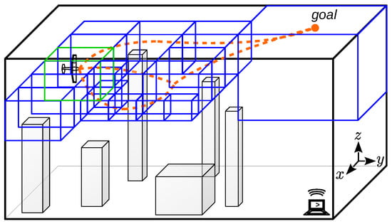
Figure 1.
General scenario for unmanned aerial vehicles (UAV) path planning. The grey cubes depict the environmental obstacles. Blue cubes are generated by the environmental discretisation and represent collision-free spaces. Orange lines are possible paths.
3. Modified Adaptive Cell Decomposition (MACD)
A standard ACD algorithm attempts to make a discrete approximation of the environment, typically in a tree data structure known as octree (Octree is a tree data structure in which each internal node has exactly eight children) []. This process requires considerable computational resources and time. The modified adaptive cell decomposition (MACD) [] does not make an exhaustive routing for each little space in the environment. If an obstacle exists, the routing in the three dimensions is in direct relation to the obstacle characteristics. The parameterised decomposition level is fixed in direct relation to the UAV manoeuvrability. This means that whenever the UAV needs a minimal space to complete a movement, this value will be defined in the level of decomposition.
Let us say denotes a discrete environment, where the set of collision-free voxels are defined as , the set of occupied voxels are defined as , and the optimal path (metric term of distance) between and as . The aim is to find the optimal path compound with a set of the nearest voxels in the space that enclose the obstacles.
The procedure is summarised in the flowchart shown in Figure 2, beginning with a specification of the number of decomposition levels. For the first level (), search limits are set to the environmental dimensions . Partition of the octree divides the environment in 8 equal parts in relation to the previous boundaries. In every single octree, an obstacle search is performed that determines the possibility of a later decomposition. Once this level decomposition is finished, the complete information of and space is completed. Finally, a planner determines the best trajectory in distance terms.
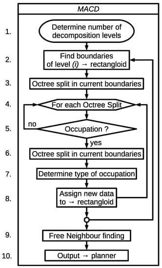
Figure 2.
Flowchart of modified adaptive cell decomposition (MACD).
A simple example in a environment is shown in Figure 3, using quadtree decomposition. The decomposition level n is predefined, n being the total levels which define the tree growth as a hierarchical computational structure. In a first segmentation, with , the environment is partitioned in underlying discrete spaces (blue lines). A second division of the environment () will generate 16 spaces (green lines).
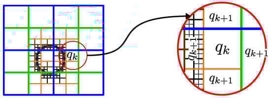
Figure 3.
Neighbourhood structure. Quadtree decomposition neighbourhood.
Figure 3 shows an example of a quadtree decomposition, denoted by with current level , with reference to its own neighbourhood. On its left side, there are neighbours with smaller dimensional characteristics than the present . There is a total of 8 neighbours, from with , of which only 8 are related directly with the neighbourhood. The lower and upper face of has the same level of decomposition, being and producing a single neighbour. On its right side, as the dimensions of the neighbour are larger than , the number of neighbours is equal to 1, counting a total of 11 neighbours and possible movements in this case.
The decomposition methodology has two relevant variations. Firstly, the definition and location of each voxel boundary, and secondly, the definition of the number of neighbours per each voxel belonging to . The number of neighbours is bounded by at least neighbours, and the maximum number of each voxel face is a multiple of with n decomposition levels (shown in Figure 4).
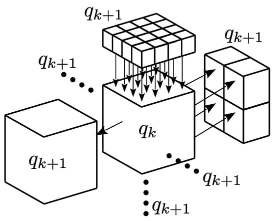
Figure 4.
Neighbourhood structure. Octree decomposition neighbourhood.
At this point, the procedure is partially complete, since the decomposition just finds the set and additional calculations to determine if are needed. Hence, MACD uses Dijkstra’s [] algorithm to calculate the optimal path in distance terms.
Algorithm 1 shows the pseudo-code to generate a structure called a rectangloid which contains all the information compiled throughout the cell decomposition process. The algorithm performs a recursive searching of the free space and the occupied space in the discrete environment to determine each voxel property (including its set of neighbours), and it simultaneously builds the computational structure that joins the voxels. For a better understanding, a brief description of several algorithm steps is offered here.
- Line 9: Boundaries of the current voxel are calculated.
- Line 12: Boundaries of the sub-voxel are assigned to rectangloid.
- Line 13: This step does a total routing by searching the environment for obstacle collisions.
- Line 24: The vertex variable collects each () of rectangloid structure.
- Line 25: The edges variable determines the structure that joins every vertex.
- Line 26:Dijkstra’s algorithm is used to determine .
| Algorithm 1 Modified Adaptive Cell Decomposition (MACD) |
|
4. Recursive Rewarding Modified Approximate Cell Decomposition (RR-MACD)
In this section, a new algorithm for path planning in environments is formulated so that using an external planner based on nodes, such as Dijkstra [] or [], becomes unnecessary. Since it attempts to achieve a final path based on starting conditions, or initial states, each future system state is determined by the present one (each state is a collision-free neighbour voxel).
4.1. Methodology
Let denote a work environment as a discrete space that contains a finite set of collision-free voxels () and a finite set of busy voxels ().
Let us assume an UAV is included within a collision-free voxel, which is considered as initial state , with the aim of reaching the end point . Let’s assume a set formed by voxels of different sizes as a neighbourhood of . In this context, a state model and a transition matrix can be developed as in Figure 5 to determine the optimal transition from to any state belonging to based on two transitional measurements and . Starting from the current state , the method will try to obtain the optimum neighbour state belonging to . It will then locate which sub-path from each neighbour in to the final point is best .
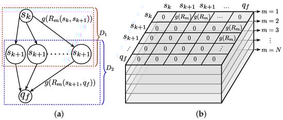
Figure 5.
Generic structure state transition. (a) Generic state model. (b) Generic transition matrix.
To solve this problem a discrete deterministic finite automaton (DDFA) [,], F, can be defined as with a set of partial functions, where:
- q are two points in the environment space, where
- -
- is the initial point
- -
- is the final point.
- S is a finite set of M current states, where
- -
- is the finite set of collision-free voxels. Split in the current voxel , and the set of its neighbours .
- -
- is the finite set of occupied voxels.
- is a set of N partial functions involved in the UAV navigation characteristics and determining feasible progress. In this paper, functions are defined as flight parameters, being:where is the Euclidean distance between any two states and is the distance in a straight line between and .where is the direction change measurement of the tangent vector to a curve, which shows the inclination angle between any two states.where is the direction change of the bi-normal vector around the tangent vector between any two states.is associated with the amount of battery and determines the possibility of success on a predefined trajectory:where is the normalised theoretical quantity of battery needed to fly from any state to any other—and the is the current amount of battery available for flight.Further, a Gaussian function is used to determine the reward in executing a possible action and it is defined as:where the transition cost values , have been normalised within boundaries . Notice how the greater the effort , the lower the reward and vice-versa. Therefore, the execution of an action from state to different states produces state transitions at different costs—an elevated cost will produce a lower reward on the transition.All these rewards can be expressed as a vector of flight parameters such as:
- is the received reward associated with a priority for executing an action on a function and is stated as the sum of two transition priority vectors and defined as:where is a predefined negative reward value in each state belonging to . Notice that the probability distribution values of the functions are independent and the set of answer vectors D which are mappings of . Therefore, this map is generated with a time-independent probability distribution. Hence, the probability of moving between one instant and the next does not change.Hence, the best reward value from vector D generates the best x—and the final path, denoted by , defines a finite labeled graph with vertex .
4.2. Simple Application
To explain the methodology, and for sake of simplicity, let’s state the problem of travelling from the actual state or point to the point in a environment using a standard cell decomposition. Figure 6a shows the initial scenario as well as the different states (observable and neighbours) that may become a new . In this case, in , it is the same cost to move right or down—this situation appears due to the inherent symmetry of the decomposition methodology. In such a situation, randomness decides the next state.
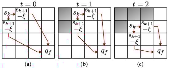
Figure 6.
Network structure and state transition. (a) state transition . (b) state transition . (c) state transition .
Since a state cannot point to itself and can be visited only once, when the states are visited and evaluated, one of them is selected by producing a forwarding movement (see Figure 6b). Hence, the state selected is the new point , and the process is repeated again (see Figure 6c). The network structure shown indicates a forward movement to the immediately next state . This movement is independent of any previous state .
Moving towards a environment, a similar scene is represented as a master voxel containing an obstacle inside (Figure 7). This voxel can be split into different levels of voxels with different dimensional characteristics in different spatial locations. To obtain the finite set of collision-free spaces , MACD is performed recursively.
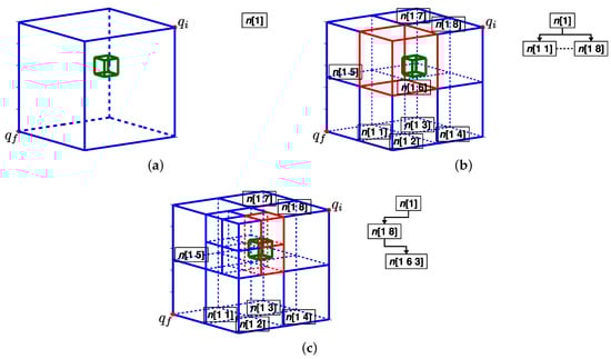
Figure 7.
Recursive rewarding MACD (RR-MACD) start process example. (a) Complete environment. (b) First MACD level . (c) second MACD Level .
The main environment boundaries have been defined from the initial coordinates to the final one , resulting in a rectangular shape, being . Each obstacle , is defined as:
where could take two possible states, static (Equation (10), the obstacle does not change its position with passing time) or dynamic (Equation (11), the obstacle changes its position to another with passing time).
Figure 7a shows the environment definition (blue lines) as the main node with an obstacle placed inside (box green lines). Once the first decomposition is performed (Figure 7b), a first octal level is generated with nodes having different occupancy properties. Each will belong to if there is no within its voxel limits () (blue lines), or to if the voxel is partial or totally occupied by the obstacle (red lines).
The first step is to determine the container voxel (for this example, it is ). In case of obstacle detection in , a recursive decomposition would be performed on the location. At this level, the node is the new starting state and the observable neighbours are the nodes , and . At this stage, the state model is depicted in Figure 8 and the transition matrix is detailed in Table 3.
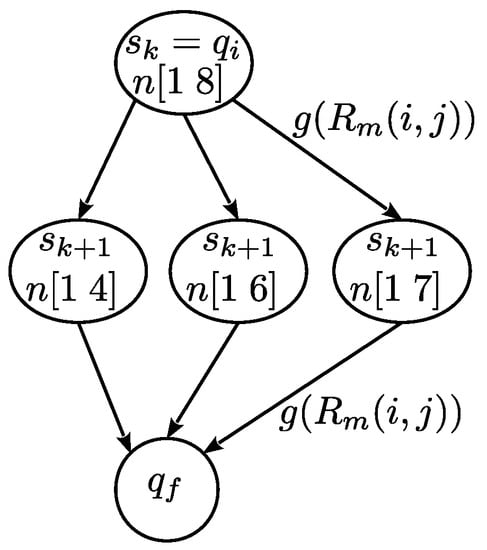
Figure 8.
State model states. List of states: .
Table 3.
Initial multidimensional transition matrix listed by first column and the first row . The number of levels are given by the number of N functions for the particular navigation characteristics.
The probability distribution for the discrete states can be derived from a multidimensional matrix of dimensions (see Table 3) where, M is the number of states, and N is the number of partial functions involved in the UAV navigation.
This multidimensional matrix equivalent to Figure 5b has been constructed with the information of the state model and the reward values. The aim is find the partial responses coming from the first row and last column, and split in two transition priority vectors . Using the priority vector and the offset , vectors and deliver partial reward distributions to a possible next state.
The transition priority vector is built with the set of columns and the row such that
The second transition priority vector, , is built with the set of rows and column .
Finally, the final reward vector D expressed as the sum of and contains the optimal value which points to the best state (node) for continuing the search of the path :
To continue with the example in Figure 7, let us assume that points to . Nevertheless, is occupied (it belongs ), so MACD is invoked, creating a new level in the data structure, composed of (see Figure 7c). Even though the state remains in , the new decomposition on returns a new set of neighbours, which join with previous ones, and define the new set defined by .
So looking for the optimum within is required. Let us assume the best node from is (notice that MACD is invoked once until now) and so the new state is reassigned to and consequently, the neighbourhood of the new state , is conformed by .
The previous actions produce the displacement from a current state to the next best state, and towards the final point. While the container voxel of the resulting better state x does not contain the point, there is the possibility that x has neighbours in different decomposition levels. Hence, the process continues until the point is reached.
Once the previous phase has been completed, the optimal path is totally determined and the search finishes. The flowchart depicted in Figure 9 and the Algorithm 2 show the pseudo-code for the described actions.
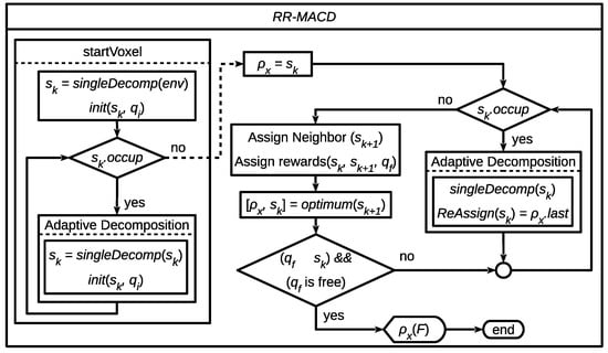
Figure 9.
Flowchart of RR-MACD. Notice how steps 3 to 8 in Figure 2 are re-used in this chart and renamed as singleDecomp.
| Algorithm 2RR-MACD |
|
The procedure is split in two stages. Firstly, a start voxel location is defined and, if there is an in the environment, an initial simple decomposition singleDecomp is performed (as a result, the collision-free voxel that contains the point will be defined). Once the initial state is assigned—which is also an initial —the procedure proceeds depending on its occupation. If is collision-free, the neighbours are assigned, the rewards are calculated, and the optimal x is located. Therefore, the best state x becomes the new and is added to . If this new is occupied, the process requires another decomposition on the current , and will return to its previous state. The procedure is completed when the current contains the point and is collision-free.
Algorithm 2 summarises the procedure described in Figure 9. In line 2, a search of the first containing is performed. The loop continues until the current state contains (line 3). If the current state collides with an obstacle , the state is decomposed (line 5: singleDecomp) and returns to its previous state (line 6). In line 8, the neighbours of , , are defined. Line 9 measures the transition rewards for any neighbour in . Finally, the optimum is added to the path and x is assigned as the new in line 10. When the loop finishes, the complete path is returned (line 13).
The methodology described presents the following properties:
- (a)
- A stochastic process in discrete time has been defined (it lacks memory), the probability distribution for a future state depends solely on its present values and is independent of the current state history.
- (b)
- The sum of the priorities defined in vector is not equal to 1. .
- (c)
- The sum of the values of each priority vector, is not equal to 1. and .
Finally, it should be noted that the environmental discrete decomposition results in ever smaller voxels of differing sizes. The level of voxel decomposition is variable based on two goals that must be fulfilled: (1) Designer defines the maximum decomposition level (minimum voxel size); however, the algorithm tries to reduce the computational cost and, as a consequence, the minimum voxel size is generally avoided. (2) As soon as a free space meets the defined constraints it is selected by the algorithm regardless of the size of the voxel.
4.3. Dynamic Environment Approach
The RR-MACD can be applied to a UAV environment with obstacles for movement. Once and points are defined, the trajectory is calculated and the UAV navigates through it. A dynamic environment implies a positional Equation (11). If the obstacles intersect the previously calculated trajectory , a new trajectory must be generated. The described methodology in the previous sections has constant targets and . However, for a dynamic trajectory the path must be updated with a new in the current UAV location.
5. Experiments
In this section, a comparison of computational performance between MACD and RR-MACD algorithms is made. Three different simulation examples have been carried out with 10 executions of each algorithm over each environment. The 150 set of responses supplies the results to determine the performance. The algorithms have been run in a “8 x Intel(R) Core(TM) i7-4790 CPU @ 3.60 GHz” computer (Manufacturer: Gigabyte Technology Co., Ltd., Model: B85M-D3H) with 8Gb RAM and S.O. Ubuntu Linux 16.04 LTS. The algorithms were programmed in MATLAB version 9.4.0.813654 (R2018a).
For each simulation example, five different 3D environments were defined. Table 4 shows one row per environment, where the column entitled "UAV target coordinates" expresses the coordinates in terms of and points. The environmental dimensions have been defined in distances related to those coordinates (in a scale of meters m). The column "Obstacles Dimensions" shows the dimensional characteristics of each obstacle and the "Obstacle Location" places the obstacles in a specific location. Moreover, the altitude between and target points are different, guaranteeing that the UAV path will be built in the axes. It should be highlighted that maps are created with predefined static obstaclesfor the different groups of experiments.
Table 4.
Definition of five different 3D environments for the simulation examples.
First, an urban environment with several buildings is described. For the construction of this environment, a maximum altitude reference has been taken, such as stated in “The Regulation of Drones in Spain 2019 [,]”. For environments defined as , and 5, larger dimensions have been considered in which a varying number of obstacles in different air spaces are defined.
5.1. Example 1. Static Obstacles and Four Flight Parameters (Constraints)
This example shows the performance of RR-MACD when four functions are used (). These functions are the same as those detailed in Section 4. In Figure 10, the specifically results for environments and are shown. Therefore, Figure 10a shows the urban environment. Hence, Figure 10b shows the built path by RR-MACD of the environment , where black boxes are the obstacles , green stars shows the voxel set of vertices in the state and the orange line shows the final path .
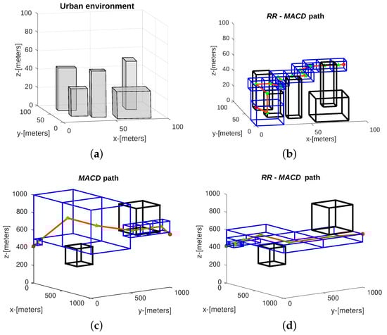
Figure 10.
Graphical Results of Example 1. (a) Modeled urban environment cluttered with surrounding buildings. (b) Results for environment with RR-MACD. (c) Final path generated using MACD for environment . (d) Final path generated using RR-MACD for environment .
In Figure 10c, the resulting MACD technique on the environment can be appreciated, where black boxes are the static obstacles , blue boxes are the set of voxels used for the Dijkstra’s planner to obtain the optimal final path (green stars are the vertices set of its belonging voxel and the orange line shows the final path . Finally, Figure 10d depicts the final trajectory built by RR-MACD, where the orange line shows the final path .
Comparisons of both algorithms regarding computational time is shown in Table 5. The results show an important advantage in decomposition time and spaces for RR-MACD. Notice that, when an obstacle intersects with a voxel decomposition, MACD recursively continues until the predefined level n (for this reason in environment the searching time for MACD is considerably greater than other environments).
Table 5.
Comparison of both algorithm executions for different environments. Column recursive rewarding modified adaptive cell decomposition (RR-MACD) 4 vs. MACD (%) shows the average resources (decomposition time (s), number of free voxel decomposition and number of nodes in the final path ) used for RR-MACD in comparison with MACD. Column RR-MACD 10 vs. RR-MACD 4 (%) shows the average resources (decomposition time (s), number of free voxels decomposition and number of nodes in the final path) used for RR-MACD when the number of flight parameters (constraints) are augmented to 10.
The third column "RR-MACD 4 vs. MACD )" shows in percentages the differences between MACD and RR-MACD 4 regarding environmental decomposition time, number of free-spaces generated during the searching process, and the number of final path nodes . It is important to mention that MACD needs an additional time because Dijks time(s) shows the seconds needed to find . For example, in the first environment, the RR-MACD algorithm just needs of the time that MACD takes for environment decomposition, and of the time that MACD takes to generate , and of the nodes that MACD needs to build . Therefore, RR-MACD shows a general improvement on the process.
5.2. Example 2. Static Obstacles and 10 Constraints
In example 1, the set of partial functions involved in UAV navigation is equal to 4. For this example, an additional set of 6 random values were added as new functions to simulate complex flight characteristics. Therefore, the number of partial functions in UAV navigation will be equal to and the probability distribution multidimensional matrix now has 10 levels. This increment of functions, and its random nature, will provoke inherent changes in the results. These can be observed in the fourth column of Table 5, entitled "RR-MACD 10 vs. RR-MACD 4 %", where the relative difference between RR-MACD 4 and RR-MACD 10 shows the percentage increase or decrease in decomposition time, and .
For example, let us compare performances between RR-MACD 10 and RR-MACD 4 in the environment . RR-MACD 10 needs more time to find a final path. It generates plus voxels and the number of nodes in the final path is higher.
Table 6 shows a set of additional data corresponding to the results in terms of distances travelled between the point and the point after the execution of each algorithm. As mentioned in the previous sections, the main objective of planning is not to reach optimality in exclusive terms of distance.
Table 6.
Path results in distance metrics.
5.3. Example 3. Dynamic Obstacles
An additional experiment was performed that considered obstacles in motion. A new environment has been proposed for obstacles intersecting with the calculated . Hence, a new with a new (actual location of the UAV) is built.
Figure 11 represents this new environment with two obstacles in motion (black boxes). The first dynamic obstacle begins its displacement in location (600, 600, 600)m, and performs a continuous motion in an direction with a constant velocity of 15 m/s. The second one begins its flight in location (80, 800, 600)m with a constant velocity of 15 m/s in the same direction. After 11 s, the first obstacle collides with (this crash is illustrated with orange line in Figure 11a) and a new is calculated, Figure 11b shows the new location of the obstacles (notice that limits in x and y axis have changed from 1000 m to 800 m). At 34 s, a new collision is detected (Figure 11c), even though the first obstacle is out of the environment, the second one has collided with . When the UAV (blue square) has passed this part of , the new trajectory until is collision-free.
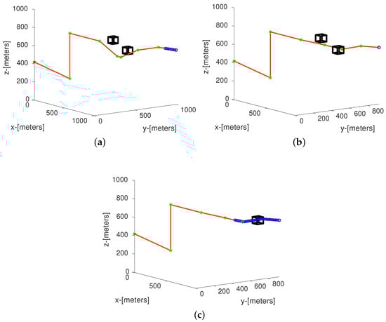
Figure 11.
Network structure and state transition. (a) Collision in time of flight . (b) New after first collision. (c) New after first collision.
6. Conclusions
This paper presents an adaptive grid methodology in environments applied to flight path planning. The approach described considers different constraints such as UAV maneuverability and geometry or static and dynamic environment obstacles.
The proposed algorithm, RR-MACD, divides the environment in a synthesised way and does not need to invoke any additional planner to search (such as Dijkstra or ) for an optimal path generation. The improvement in the computational effort and the reduction in the number of nodes generated by the RR-MACD has been shown. The stochastic process in discrete time involved in the algorithm also shows a future probability distribution that only depends on its present states.
The partition of the space into a defined geometric form enables decreasing the number of control points in the generated trajectory. In addition, the issue of computational cost and complexity has been addressed by providing a solution that generates relatively shorter time responses compared to techniques for generating similar trajectories.
In a future work, an additional processing task will be carried out, using the set of nodes, or control points generated, to create a smoother path—and then the methodology will be tested under real flight conditions on an UAV model as in [,,].
Author Contributions
Conceptualization, F.S.; Formal analysis, F.S., J.S., S.G.-N. and R.S.; Methodology, F.S.; Supervision, J.S., S.G.-N. and R.S.
Funding
The authors would like to acknowledge the Spanish Ministry of Economy and Competitiveness for providing funding through the project DPI2015-71443-R and the local administration Generalitat Valenciana through the project GV/2017/029. Franklin Samaniego thanks IFTH (Instituto de Fomento al Talento Humano) Ecuador (2015-AR2Q9209), for its sponsorship of this work.
Acknowledgments
The authors would like to thank the editors and the reviewers for their valuable time and constructive comments.
Conflicts of Interest
The authors declare no conflict of interest.
References
- Valavanis, K.; Vachtsevanos, G. Handbook of Unmanned Aerial Vehicles; Springer: Dordrecht, The Netherlands, 2015; pp. 2993–3009. [Google Scholar] [CrossRef]
- 20 Great UAV Applications Areas for Drones. Available online: http://air-vid.com/wp/20-great-uav-applications-areas-drones/ (accessed on 28 December 2018).
- Industry Experts—Microdrones. Available online: https://www.microdrones.com/en/industry-experts/ (accessed on 28 December 2018).
- Rodríguez, R.; Alarcón, F.; Rubio, D.; Ollero, A. Autonomous Management of an UAV Airfield. In Proceedings of the 3rd International Conference on Application and Theory of Automation in Command and Control Systems, Naples, Italy, 28–30 May 2013; pp. 28–30. [Google Scholar]
- Li, J.; Han, Y. Optimal Resource Allocation for Packet Delay Minimization in Multi-Layer UAV Networks. IEEE Commun. Lett. 2017, 21, 580–583. [Google Scholar] [CrossRef]
- Stuchlík, R.; Stachoň, Z.; Láska, K.; Kubíček, P. Unmanned Aerial Vehicle—Efficient mapping tool available for recent research in polar regions. Czech Polar Rep. 2015, 5, 210–221. [Google Scholar] [CrossRef]
- Pulver, A.; Wei, R. Optimizing the spatial location of medical drones. Appl. Geogr. 2018, 90, 9–16. [Google Scholar] [CrossRef]
- Claesson, A.; Svensson, L.; Nordberg, P.; Ringh, M.; Rosenqvist, M.; Djarv, T.; Samuelsson, J.; Hernborg, O.; Dahlbom, P.; Jansson, A.; et al. Drones may be used to save lives in out of hospital cardiac arrest due to drowning. Resuscitation 2017, 114, 152–156. [Google Scholar] [CrossRef] [PubMed]
- Reineman, B.; Lenain, L.; Statom, N.; Melville, W. Development and Testing of Instrumentation for UAV-Based Flux Measurements within Terrestrial and Marine Atmospheric Boundary Layers. J. Atmos. Ocean. Technol. 2013, 30, 1295–1319. [Google Scholar] [CrossRef]
- Hernández, E.; Vázquez, M.; Zurro, M. Álgebra lineal y Geometría, 3rd ed.; Pearson: Upper Saddle River, NJ, USA, 2012. [Google Scholar]
- LaValle, S. Planning Algorithms; Cambridge University Press: Cambridge, UK, 2006; pp. 1–826. [Google Scholar] [CrossRef]
- Elbanhawi, M.; Simic, M. Sampling-Based Robot Motion Planning: A Review. IEEE Access 2014, 2, 56–77. [Google Scholar] [CrossRef]
- Hernandez, K.; Bacca, B.; Posso, B. Multi-goal path planning autonomous system for picking up and delivery tasks in mobile robotics. IEEE Lat. Am. Trans. 2017, 15, 232–238. [Google Scholar] [CrossRef]
- Kohlbrecher, S.; Von Stryk, O.; Meyer, J.; Klingauf, U. A flexible and scalable SLAM system with full 3D motion estimation. In Proceedings of the 9th IEEE International Symposium on Safety, Security, and Rescue Robotics SSRR 2011, Tokyo, Japan, 22–24 August 2011; pp. 155–160. [Google Scholar] [CrossRef]
- Abbadi, A.; Matousek, R.; Jancik, S.; Roupec, J. Rapidly-exploring random trees: 3D planning. In Proceedings of the 18th International Conference on Soft Computing MENDEL, Brno, Czech Republic, 27–29 June 2012; pp. 594–599. [Google Scholar]
- Aguilar, W.; Morales, S. 3D Environment Mapping Using the Kinect V2 and Path Planning Based on RRT Algorithms. Electronics 2016, 5, 70. [Google Scholar] [CrossRef]
- Aguilar, W.; Morales, S.; Ruiz, H.; Abad, V. RRT* GL Based Optimal Path Planning for Real-Time Navigation of UAVs. Soft Comput. 2017, 17, 585–595. [Google Scholar] [CrossRef]
- Yao, P.; Wang, H.; Su, Z. Hybrid UAV path planning based on interfered fluid dynamical system and improved RRT. In Proceedings of the IECON 2015—41st Annual Conference of the IEEE Industrial Electronics Society, Yokohama, Japan, 9–12 November 2015; pp. 829–834. [Google Scholar] [CrossRef]
- Yan, F.; Liu, Y.; Xiao, J. Path Planning in Complex 3D Environments Using a Probabilistic Roadmap Method. Int. J. Autom. Comput. 2013, 10, 525–533. [Google Scholar] [CrossRef]
- Yeh, H.; Thomas, S.; Eppstein, D.; Amato, N. UOBPRM: A uniformly distributed obstacle-based PRM. In Proceedings of the 2012 IEEE/RSJ International Conference on Intelligent Robots and Systems, Vilamoura, Algarve, Portugal, 7–12 October 2012; pp. 2655–2662. [Google Scholar] [CrossRef]
- Denny, J.; Amatoo, N. Toggle PRM: A Coordinated Mapping of C-Free and C-Obstacle in Arbitrary Dimension. Algorithm. Found. Robot. X 2013, 86, 297–312. [Google Scholar] [CrossRef]
- Li, Q.; Wei, C.; Wu, J.; Zhu, X. Improved PRM method of low altitude penetration trajectory planning for UAVs. In Proceedings of the 2014 IEEE Chinese Guidance, Navigation and Control Conference, Yantai, China, 8–10 August 2014; pp. 2651–5656. [Google Scholar] [CrossRef]
- Ortiz-Arroyo, D. A hybrid 3D path planning method for UAVs. In Proceedings of the 2015 Workshop on Research, Education and Development of Unmanned Aerial Systems (RED-UAS), Cancún, México, 23–25 November 2015; pp. 123–132. [Google Scholar] [CrossRef]
- Thanou, M.; Tzes, A. Distributed visibility-based coverage using a swarm of UAVs in known 3D-terrains. In Proceedings of the 2014 6th International Symposium on Communications, Control and Signal Processing (ISCCSP), Athens, Greece, 21–23 May 2014; pp. 425–428. [Google Scholar] [CrossRef]
- Qu, Y.; Zhang, Y.; Zhang, Y. Optimal flight path planning for UAVs in 3-D threat environment. In Proceedings of the 2014 International Conference on Unmanned Aircraft Systems (ICUAS), Orlando, FL, USA, 27–30 May 2014; pp. 149–155. [Google Scholar] [CrossRef]
- Fang, Z.; Luan, C.; Sun, Z. A 2D Voronoi-Based Random Tree for Path Planning in Complicated 3D Environments. Intell. Auton. Syst. 2017, 531, 433–445. [Google Scholar] [CrossRef]
- Khuswendi, T.; Hindersah, H.; Adiprawita, W. UAV path planning using potential field and modified receding horizon A* 3D algorithm. In Proceedings of the 2011 International Conference on Electrical Engineering and Informatics, Bandung, Indonesia, 17–19 July 2011; pp. 1–6. [Google Scholar] [CrossRef]
- Chen, X.; Zhang, J. The Three-Dimension Path Planning of UAV Based on Improved Artificial Potential Field in Dynamic Environment. In Proceedings of the 2013 5th International Conference on Intelligent Human-Machine Systems and Cybernetics, Hangzhou, Zhejiang, China, 26–27 August 2013; Volume 2, pp. 144–147. [Google Scholar] [CrossRef]
- Rivera, D.; Prieto, F.; Ramirez, R. Trajectory Planning for UAVs in 3D Environments Using a Moving Band in Potential Sigmoid Fields. In Proceedings of the 2012 Brazilian Robotics Symposium and Latin American Robotics Symposium, Fortaleza, Ceara, Brazil, 16–19 October 2012; pp. 115–119. [Google Scholar] [CrossRef]
- Liu, L.; Shi, R.; Li, S.; Wu, J. Path planning for UAVS based on improved artificial potential field method through changing the repulsive potential function. In Proceedings of the 2016 IEEE Chinese Guidance, Navigation and Control Conference (CGNCC), Nanjing, China, 12–14 August 2016; pp. 2011–2015. [Google Scholar] [CrossRef]
- Dijkstra, E. A note on two problems in connexion with graphs. Numer. Math. 1959, 1, 269–271. [Google Scholar] [CrossRef]
- Verscheure, L.; Peyrodie, L.; Makni, N.; Betrouni, N.; Maouche, S.; Vermandel, M. Dijkstra’s algorithm applied to 3D skeletonization of the brain vascular tree: Evaluation and application to symbolic. In Proceedings of the 2010 Annual International Conference of the IEEE Engineering in Medicine and Biology, Buenos Aires, Argentina, 31 August–4 September 2010; pp. 3081–3084. [Google Scholar] [CrossRef]
- Hart, P.E.; Nils, J. A formal basis for the Heuristic Determination of minimum cost paths. IEEE Trans. Syst. Sci. Cybern. 1968, 4, 100–107. [Google Scholar] [CrossRef]
- Niu, L.; Zhuo, G. An Improved Real 3D a* Algorithm for Difficult Path Finding Situation. In Proceedings of the International Archives of the Photogrammetry, Remote Sensing and Spatial Information Sciences, Beijing, China, 3–11 July 2008; Volume 37, pp. 927–930. [Google Scholar]
- Stentz, A. Optimal and Efficient Path Planning for Partially-Known Environments. ICRA 1994, 94, 3310–3317. [Google Scholar]
- Ferguson, D.; Stentz, A. Field D*: An Interpolation-Based Path Planner and Replanner. Robot. Res. 2007, 28, 239–253. [Google Scholar] [CrossRef]
- De Filippis, L.; Guglieri, G.; Quagliotti, F. Path Planning Strategies for UAVS in 3D Environments. J. Intell. Robotic Syst. 2012, 65, 247–264. [Google Scholar] [CrossRef]
- Nosrati, M.; Karimi, R.; Hasanvand, H. Investigation of the * (Star) Search Algorithms: Characteristics, Methods and Approaches. World Appl. Program. 2012, 2, 251–256. [Google Scholar]
- Kroumov, V.; Yu, J.; Shibayama, K. 3D path planning for mobile robots using simulated annealing neural network. In Proceedings of the 2009 International Conference on Networking, Sensing and Control, Okayama, Japan, 29 March 2009; pp. 130–135. [Google Scholar]
- Gautam, S.; Verma, N. Path planning for unmanned aerial vehicle based on genetic algorithm & artificial neural network in 3D. In Proceedings of the 2014 International Conference on Data Mining and Intelligent Computing (ICDMIC), Odisha, India, 20–21 December 2014; pp. 1–5. [Google Scholar] [CrossRef]
- Maturana, D.; Scherer, S. 3D Convolutional Neural Networks for landing zone detection from LiDAR. In Proceedings of the 2015 IEEE International Conference on Robotics and Automation (ICRA), Beijing, China, 2–5 August 2015; Volume 2015, pp. 3471–3478. [Google Scholar] [CrossRef]
- Iswanto, I.; Wahyunggoro, O.; Cahyadi, A. Quadrotor Path Planning Based on Modified Fuzzy Cell Decomposition Algorithm. TELKOMNIKA Telecommun. Comput. Electron. Control 2016, 14, 655–664. [Google Scholar] [CrossRef]
- Liu, S.; Wei, Y.; Gao, Y. 3D path planning for AUV using fuzzy logic. In Proceedings of the Computer Science and Information Processing (CSIP)), Xi’an, Shaanxi, China, 24–26 August 2012; pp. 599–603. [Google Scholar]
- Duan, H.; Yu, Y.; Zhang, X.; Shao, S. Three-dimension path planning for UCAV using hybrid meta-heuristic ACO-DE algorithm. Simul. Model. Pract. Theory 2010, 18, 1104–1115. [Google Scholar] [CrossRef]
- He, Y.; Zeng, Q.; Liu, J.; Xu, G.; Deng, X. Path planning for indoor UAV based on Ant Colony Optimization. In Proceedings of the 2013 25th Chinese Control and Decision Conference (CCDC), Guiyang, China, 25–27 May 2013; pp. 2919–2923. [Google Scholar] [CrossRef]
- Zhang, Y.; Wu, L.; Wang, S. UCAV Path Planning by Fitness-Scaling Adaptive Chaotic Particle Swarm Optimization. Math. Probl. Eng. 2013, 1–9. [Google Scholar] [CrossRef]
- Goel, U.; Varshney, S.; Jain, A.; Maheshwari, S.; Shukla, A. Three Dimensional Path Planning for UAVs in Dynamic Environment using Glow-worm Swarm Optimization. Procedia Comput. Sci. 2013, 133, 230–239. [Google Scholar] [CrossRef]
- Chen, Y.; Mei, Y.; Yu, J.; Su, X.; Xu, N. Three-dimensional unmanned aerial vehicle path planning using modified wolf pack search algorithm. Neurocomputing 2017, 226, 4445–4457. [Google Scholar] [CrossRef]
- Wang, G.; Chu, H.E.; Mirjalili, S. Three-dimensional path planning for UCAV using an improved bat algorithm. Aerosp. Sci. Technol. 2016, 49, 231–238. [Google Scholar] [CrossRef]
- Aghababa, M. 3D path planning for underwater vehicles using five evolutionary optimization algorithms avoiding static and energetic obstacles. Appl. Ocean Res. 2012, 38, 48–62. [Google Scholar] [CrossRef]
- Mac, T.; Copot, C.; Tran, D.; De Keyser, R. Heuristic approaches in robot path planning: A survey. Rob. Auton. Syst. 2016, 86, 13–28. [Google Scholar] [CrossRef]
- Szirmay-Kalos, L.; Márton, G. Worst-case versus average case complexity of ray-shooting. Computing 1998, 61, 103–131. [Google Scholar] [CrossRef]
- Berger, M.J.; Oliger, J. Adaptive mesh refinement for hyperbolic partial differential equations. Comput. Phys. 1984, 53, 484–512. [Google Scholar] [CrossRef]
- Min, C.; Gibou, F. A second order accurate projection method for the incompressible Navier-Stokes equations on non-graded adaptive grids. J. Comput. Phys. 2006, 219, 912–929. [Google Scholar] [CrossRef]
- Hasbestan, J.J.; Senocak, I. Binarized-octree generation for Cartesian adaptive mesh refinement around immersed geometries. J. Comput. Phys. 2018, 368, 179–195. [Google Scholar] [CrossRef]
- Pantano, C.; Deiterding, R.; Hill, D.J.; Pullin, D.I. A low numerical dissipation patch-based adaptive mesh refinement method for large-eddy simulation of compressible flows. J. Comput. Phys. 2007, 221, 3–87. [Google Scholar] [CrossRef]
- Ryde, J.; Hu, H. 3D mapping with multi-resolution occupied voxel lists. Auton. Robots 2010, 28, 169–185. [Google Scholar] [CrossRef]
- Samet, H.; Kochut, A. Octree approximation an compression methods. In Proceedings of the First International Symposium on 3D Data Processing Visualization and Transmission, Padova, Italy, 19–21 June 2002; pp. 460–469. [Google Scholar] [CrossRef]
- Samaniego, F.; Sanchis, J.; García-Nieto, S.; Simarro, R. UAV motion planning and obstacle avoidance based on adaptive 3D cell decomposition: Continuous space vs discrete space. In Proceedings of the 2017 IEEE Ecuador Technical Chapters Meeting (ETCM), Salinas, Ecuador, 6–20 October 2017; pp. 1–6. [Google Scholar] [CrossRef]
- Markus, S.; Akesson, K.; Martin, F. Modeling of discrete event systems using finite automata with variables. In Proceedings of the 2007 46th IEEE Conference on Decision and Control, New Orleans, LA, USA, 12–14 December 2007; pp. 3387–3392. [Google Scholar] [CrossRef]
- Yang, Y.; Prasanna, V. Space-time tradeoff in regular expression matching with semi-deterministic finite automata. In Proceedings of the 2011 IEEE INFOCOM, Shanghai, China, 17 August 2007; pp. 1853–1861. [Google Scholar] [CrossRef]
- Normativa Sobre Drones en España [2019]—Aerial Insights. Available online: http://www.aerial-insights.co/blog/normativa-drones-espana/ (accessed on 28 December 2018).
- Disposición 15721 del BOE núm. 316 de 2017 - BOE.es. Available online: https://www.boe.es/boe/dias/2017/12/29/pdfs/BOE-A-2017-15721.pdf (accessed on 28 December 2018).
- Velasco-Carrau, J.; García-Nieto, S.; Salcedo, J.; Bishop, R. Multi-Objective Optimization for Wind Estimation and Aircraft Model Identification. J. Guid. Control Dyn. 2016, 39, 372–389. [Google Scholar] [CrossRef]
- Vanegas, G.; Samaniego, F.; Girbes, V.; Armesto, L.; Garcia-Nieto, S. Smooth 3D path planning for non-holonomic UAVs. In Proceedings of the 2018 7th International Conference on Systems and Control (ICSC), València, Spain, 24–26 October 2018; pp. 1–6. [Google Scholar] [CrossRef]
- Samaniego, F.; Sanchís, J.; García-Nieto, S.; Simarro, R. Comparative Study of 3-Dimensional Path Planning Methods Constrained by the Maneuverability of Unmanned Aerial Vehicles. In Proceedings of the 2018 7th International Conference on Systems and Control (ICSC), València, Spain, 24–26 October 2018; pp. 13–20. [Google Scholar] [CrossRef]

© 2019 by the authors. Licensee MDPI, Basel, Switzerland. This article is an open access article distributed under the terms and conditions of the Creative Commons Attribution (CC BY) license (http://creativecommons.org/licenses/by/4.0/).