1. Introduction
Deep convolutional neural networks (DCNNs) [
1] have shown significant advantages in many artificial intelligence (AI) applications, such as computer vision and natural language processing [
2,
3,
4]. The performance of the DCNN is improving rapidly: the winner of ImageNet classification has promoted the top-1 classification accuracy from 57.2% in 2012 (AlexNet) to 76.1% in 2015 (ResNet-152) [
5,
6]. However, this accuracy improvement is achieved at the expense of higher computational complexity first. For example, AlexNet takes 1.4 GOPS to process a single 224 × 224 image, while ResNet-152 consumes 22.6 GOPS. The traditional central processing unit (CPU) platform has difficulty in satisfying the computing requirements of a convolutional neural network (CNN). Another key challenge is the energy consumption. Although the graphics processing unit (GPU) shows a strong parallel computing performance for accelerating the CNN [
7], the excessive power consumption limits their application potential. The GPU has an advantage in accelerating the training phase of the CNN without considering power-hungry and volume-constrained problems, while a field programmable gate array (FPGA) and an application specific integrated circuit (ASIC) are suitable for accelerating the inference phase of the CNN with limited hardware resources and tight power budgets [
8,
9,
10]. Though the ASIC has both excellent performance and energy efficiency, it suffers from low flexibility, high development costs, and a long development cycle.
The FPGA has shown excellent performance, especially energy efficiency and flexibility in accelerating deep learning. Farabet exploits the inherent parallelism of the CNN and takes full advantage of multiple hardware multiply accumulate units on the FPGA [
11]. A scalable dataflow hardware architecture is optimized for the computation of general-purpose vision algorithms [
12]. Meng develops a deep model, termed the Gabor CNN, to address the computing-resource-saving problem [
13]. Liu proposes a uniform architecture design by mapping convolutions to matrix multiplications for accelerating both two dimensional (2D) and three dimensional (3D) CNNs [
14]. Despite the progress made, those accelerators take the algorithm as a black box, only focusing on hardware architecture optimization. Different from the previous approaches, Han presents the “deep compression” and “efficient speech recognition engine” (ESE) to support sparse recurrent neural networks (RNNs) and long short-term memory networks (LSTMs) [
15,
16,
17], and also provides the “efficient inference engine” (EIE) to perform inference on the compressed DNNs [
18]. These software-hardware co-designs show great advantages in accelerating deep learning, but there is still a lack of analysis on the connection between the fully connected layer and the convolutional layer, leaving plenty of room for algorithm optimization.
From the hardware perspective, a compressed CNN model requires less computation and memory, indicating a great potential to improve speed and energy efficiency. However, the model compression algorithm makes the computation pattern irregular, and the conventional FPGA-based accelerators are optimized for uncompressed CNN models, resulting in huge wastes of computation cycles and memory bandwidth compared with running on compressed CNN models.
In this paper, we propose an optimized compression strategy, and implement an efficient FPGA-based accelerator for a compressed CNN. Firstly, we present the reversed-pruning and peak-pruning method, respectively, which significantly reduces the number of parameters without affecting the accuracy. Secondly, quantization is applied to decrease precision and bit width with negligible loss of accuracy, aggravating more zero weights and one weights. Thirdly, an efficient storage method for the convolutional layer and the fully connected layer is proposed to reduce the occupancy of the whole overhead cache, separately. Finally, we design an accelerator for a compressed CNN based on the Xilinx Zynq FPGA. In order to verify the performance, we implement the compressed AlexNet on the Xilinx ZCU104 evaluation board using Xilinx SDx IDE tools and the Vivado 2018.2 system suite.
The paper is organized as follows:
Section 2 provides the background for model compression.
Section 3 presents our optimized model compression techniques, including the reversed-pruning, peak-pruning, and quantization, and then efficient storage is proposed for reducing overhead cache. Efficient FPGA-based accelerator for the compressed CNN and its main components are designed in
Section 4.
Section 5 describes the performance of our accelerator compared with similar FPGA implementations, and
Section 6 concludes the paper.
2. Motivation for Compressing CNNs
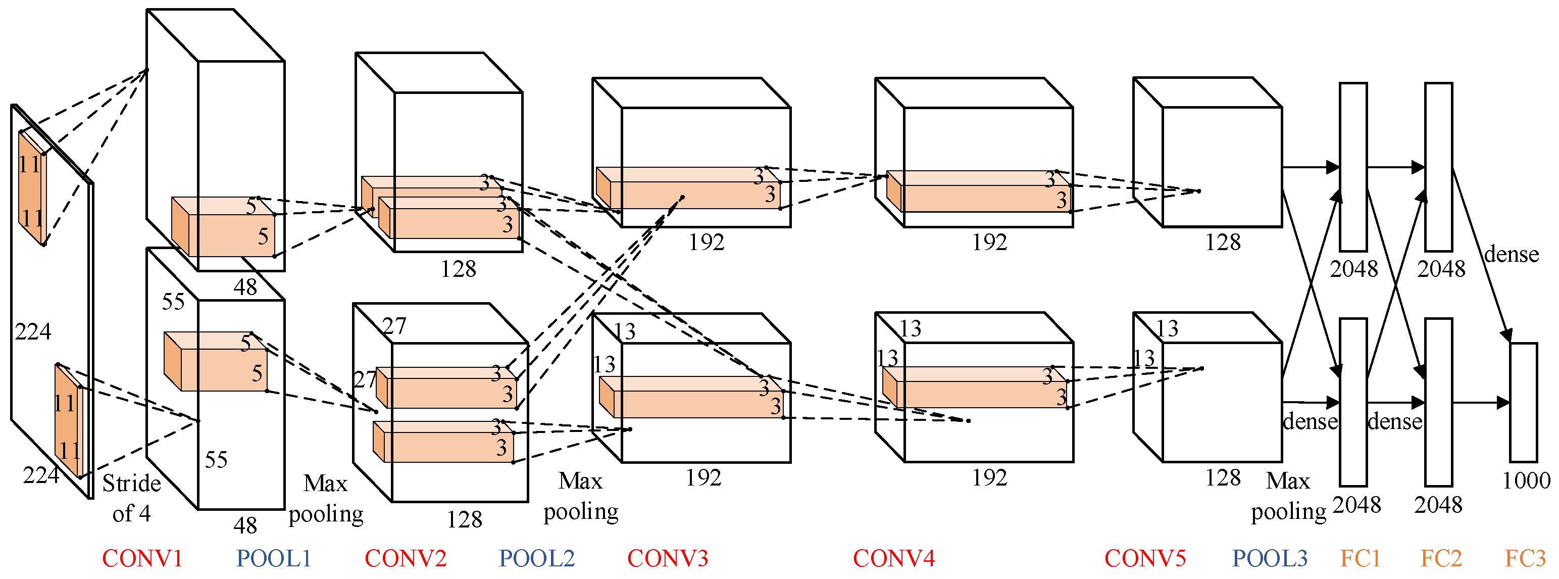
A typical CNN is shown in
Figure 1, consisting of several layers running in sequence from CONV1 to FC3 [
19]. The first layer of a CNN reads an input image and outputs a series of feature maps. After that, a layer reads the feature maps generated by the previous layers and outputs new feature maps. Finally, a classifier outputs the probability of each category that the input image might belong to. The convolutional (CONV) layer and fully connected (FC) layer are two essential types of layer in CNNs. The AlexNet consists of five FC layers and three CONV layers. There is always one pooling (POOL) layer behind the FC layer.
After many years of development, the state-of-the-art CNN models are much more advanced than the early ones. Growing larger and deeper, the large number of parameters consume considerable storage, memory bandwidth, and computational resources which cannot be ignored for practical applications [
20]. In addition, neural networks are typically over-fitting, causing serious redundancy for CNN models [
21,
22]. In this paper, the goal is to compress a large CNN to run inference within acceptable loss of accuracy. The smaller the CNN model is, the less storage will be consumed, leading to less calculation amounts and higher inference speeds.
3. Model Compression
There are two directions to compress the network: reducing the number of weights and decreasing the precision (fewer bits per weight). After thorough investigation of the difference and connection between the convolutional layer and the fully connected layer, we proposed a reversed-pruning and peak-pruning strategy to reduce the number of weights. Further, we quantized the pruned CNN model to lower precision. After quantization, the weights of the convolutional layer and the fully connected layer were stored in a completely different way according to their respective data structures, making less overhead for memory.
3.1. Reversed-Pruning and Peak-Pruning
The reversed-pruning approach we proposed was inspired by Han’s work [
15]. Network pruning is to prune low-weight connections, removing all connections below certain thresholds with little contribution to the network’s result. Reversed-pruning means pruning weights layer by layer, from the last layer to the first. Based on this, we present the peak-pruning strategy. The novelty is that peak-pruning signifies pruning weights layer by layer from the largest number of parameters to the smallest. As shown in
Table 1, the AlexNet runs from CONV1 to FC3 in sequence. Therefore, reversed-pruning means pruning weights from FC3 to CONV1, while peak-pruning means pruning weights from FC1 to CONV1, because FC1 has the most 17 M parameters and CONV1 has the fewest 35 K parameters.
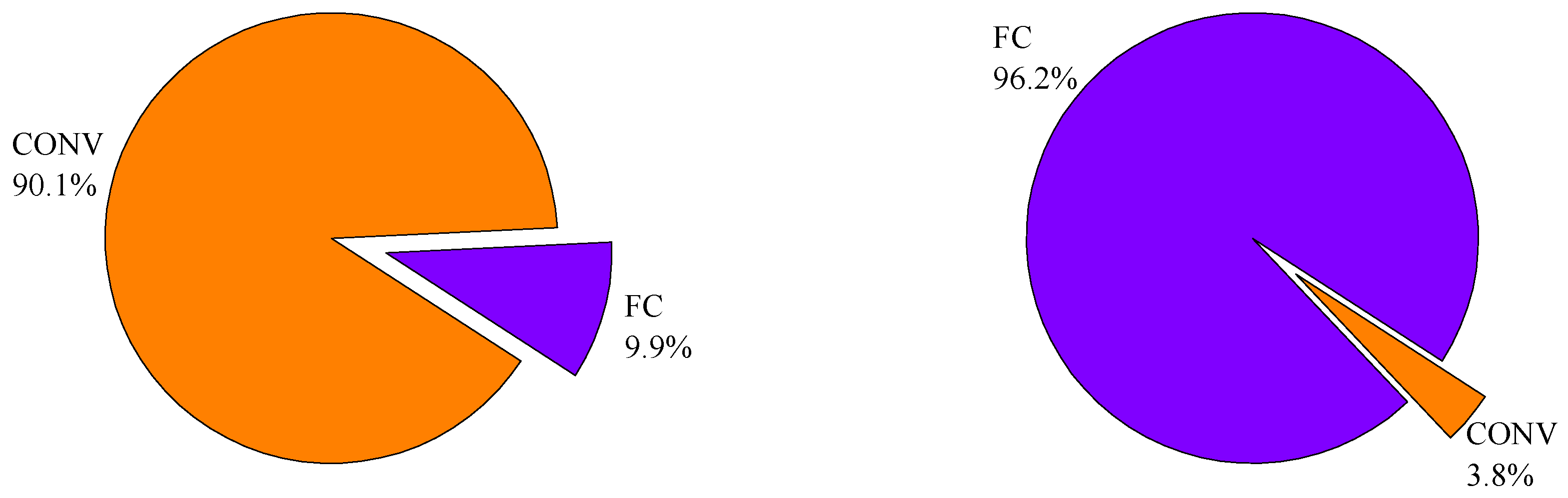
The essence of the convolutional layer is the feature extractor, while for the fully connected layer it is the classifier. The feature extractor extracts different features from input images, including lines, corners, circular arch, etc., which are relatively invariant to distortions or position shifting. Absolutely, the convolutional layer has a hungry-computation demand. The classifier is based on multi-layer perceptron (MLP). The function of the classifier is to integrate these different features from the feature extractor to decide the likelihood of categories that the input image may belong to. Conversely, the fully connected layer has a heavy-memory demand. In general, the convolutional layers take up less than 10% of the total network weights but occupy more than 90% of the computation time, while the fully connected layers take up more than 90% of the total network weights but occupy less than 10% of the computation time.
Figure 2 illustrates the unbalanced demand for computation and memory of the AlexNet inference. AlexNet has 61 M weights and takes 1.45 GOPS to process a single 224 × 224 image. The CONV layers of AlexNet have 2 M weights and take 1.33 GOPS computation, while the FC layers of AlexNet occupy 59 M weights and take 0.12 GOPS computation.
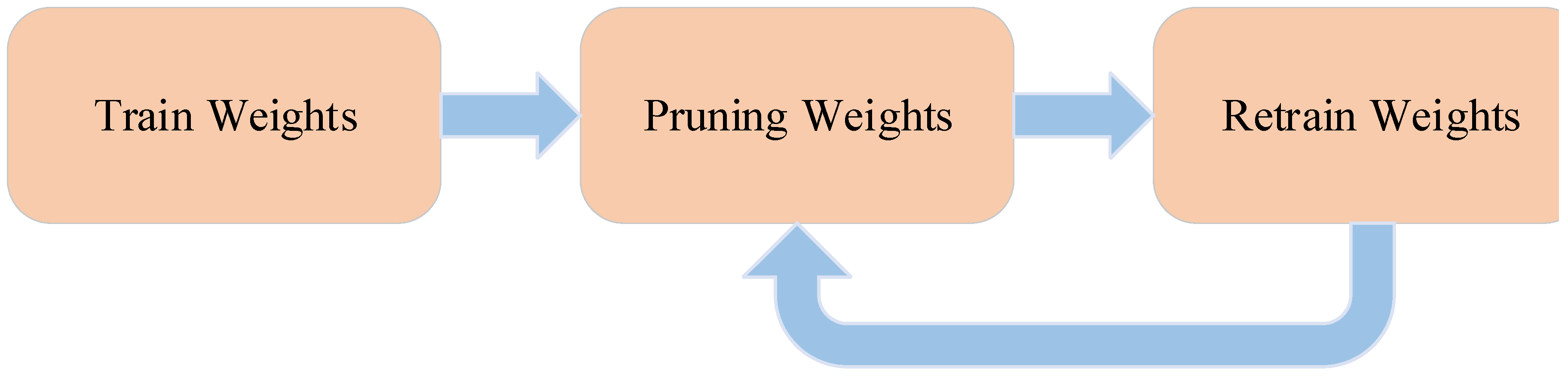
Considering that the fully connected layer is more over-parameterized and has aggressive pruning compared with the convolutional layer, our pruning strategy implements a three-step pipeline process, as illustrated in
Figure 3, which starts from adjusting weights via conventional network training. The second step prunes the weights below the threshold into zeroes, converting an originally dense network into a sparse one. The final step is to retrain the remaining non-zero weights to adapt to the forced zero weights, otherwise the accuracy will be significantly affected. Such network pruning is performed iteratively layer by layer: after pruning and retraining one layer of the CNN to achieve the original accuracy, the next layer will be pruned and retrained until all layers are completely pruned.
The proposed reversed-pruning and peak-pruning can achieve better compressibility 13× for AlexNet contrasted with Han’s 9× without harming the original accuracy. The original AlexNet Caffe model achieves a top-1 accuracy of 57.13% on ImageNet. The detailed sparsity of each layer and final accuracy after retraining are shown in
Table 2. It should be noted that the final accuracy of reversed-pruning corresponds to the CONV1 pruning because CONV1 is the last layer in reverse order, while the final accuracy of peak-pruning corresponds to the CONV1 pruning because CONV1 has the fewest parameters. In addition, layers are not independent from each other, but closely correlated. It can be seen that the fully connected layers have lower sparsity in peak-pruning relatively, while the convolutional layers have lower sparsity in reverse-pruning.
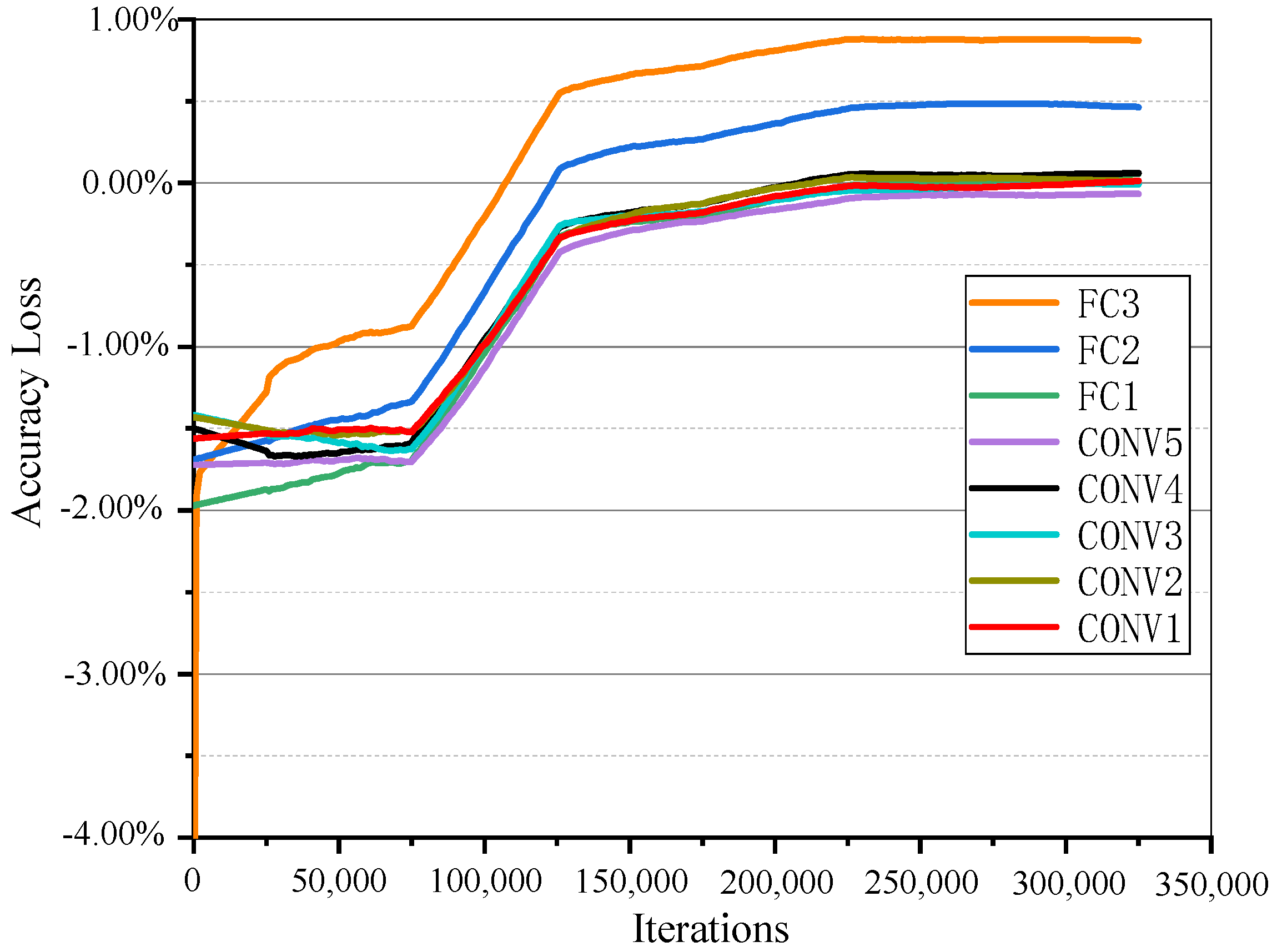
The detailed retraining process per sparse layer of AlexNet is shown in
Figure 4. The
y axis denotes the accuracy loss, which is relative to the top-1 accuracy 57.13% of the original model. As illustrated in Equation (1), the accuracy loss exhibits as negative values, which indicates that the accuracy after pruning and retraining does not recover the original accuracy. The
x axis indicates the number of iterations. It can be seen that the classification accuracy was seriously damaged after each pruning. In addition, not all layers restore to the original accuracy after retraining. One reason is that the preceding layers for pruning should leave some redundancy for the pruning of the following layers. The other is that the latter layers use conservative pruning to compensate for the accuracy loss caused by the previous layer of aggressive pruning. For example, the retrained accuracy of FC3 and FC2 was much higher than the original value while CONV4 and CONV3 were slightly lower. Ultimately, the CONV1, represented by the red line in
Figure 4, was the last retraining process, and the retrained accuracy of which was higher than the original AlexNet model.
Given that activation sparsity occurs due to the rectified linear unit (ReLU) function which is commonly used as the non-linear operator in CNNs, forcing all negatively valued activations to be clamped to zeroes. As shown in
Figure 5, the left
y axis denotes the weight and input activation sparsity of each layer of the AlexNet, and the right one indicates the ideal number of multiplication and accumulation (MAC) that could be achieved if all multiplies with a zero operand were eliminated. This is calculated by taking the product of the weight and input activation sparsity per layer.
3.2. Data Quantization
We further compressed the model by quantizing bit-width per weight from a 32-bits float point into 8-bits, making it more efficient to implement MAC operations on FPGA. That is because image processing tasks are insensitive to numerical accuracy, and FPGA is more suitable for data processing with 8-bit precision. It has been proven that quantization has very little impact on image processing [
23,
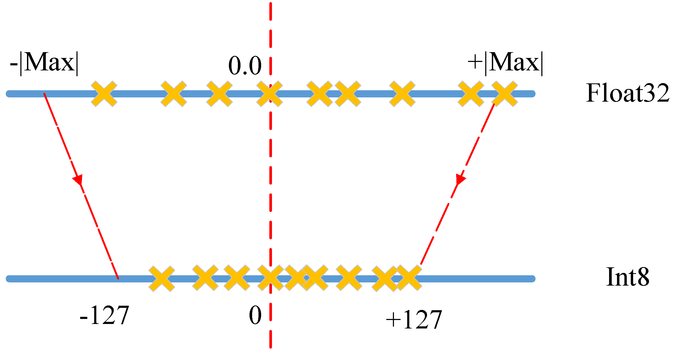
24]. We designed a linear maximum quantization strategy for each layer in the pruned CNN, as shown in
Figure 6. The linear maximum quantization was to sort the weight range of each layer in the pruned CNN, and then take the maximum absolute value as the threshold and map the range directly to the int8 scale. It should be noted that when the positive and negative distribution was not uniform, there was a part of the vacancy, but this method maximized the original information.
Another benefit of data quantization is that it introduces more zeros and one values on top of the pruning, making the pruned CNN more sparse. As is shown in
Table 3, the pruned AlexNet can be quantized to 8-bits for each layer with a negligible 1% loss of accuracy, reducing 4× less storage and computation amount. Han [
15] quantifies weights of the CONV layer with 8 bits and the FC layer with 5 bits for less storage, but the 5-bit precision is not effective for hardware implementation. In addition, our quantization does not require any additional fine tuning or retraining, and neither the codebook nor the index exists, reducing the overhead to recover the quantized sparse weight matrix.
3.3. Efficient Storage
Pruning makes the original dense weight matrix sparse, and extra space is required to store the index of non-zero weights. Though quantization has lower precision, it does not need extra storage for the codebook and index. Hence, for the quantized sparse weight matrix, only non-zero weights and their indices should be stored. In order to obtain higher storage efficiency, we developed efficient storage methods for the characteristics of the convolutional layer and fully connected layer, respectively, to reduce the overhead cache and data movement.
For the convolutional layer, the input was a combination of several 2D feature maps. After pruning and quantization, these 2D feature maps were converted into a series of quantized sparse matrices. The quantized non-zero weights and their indices were stored then. The common sparse matrix storage formats included coordinate (COO), compressed sparse row (CSR), and compressed sparse column (CSC). The CSR and CSC formats require three arrays, totally 2a + n + 1 numbers, where a is the number of non-zero elements and n is the number of rows or columns. The COO format requires three arrays and totally 3a numbers without requirement for extra computation to recover the original sparse matrix, in contrast to CSR and CSC. Considering the general convolutional kernel sizes of 11 × 11, 5 × 5, 3 × 3, and 1 × 1, the 4-bit width was enough to denote the rows’ or columns’ indices. We propose the compressed coordinate (CCOO) format, which requires two arrays, totally 2a numbers. One array is for the non-zero values, and the other is for its 8-bit indices consisting of high 4-bit row indices and low 4-bit column indices.
Table 4 shows a detailed comparison of different sparse matrix storage formats. Taking the CONV1 of the quantized pruned AlexNet as an example, the convolutional kernels size was 11 × 11 and the sparsity was 0.23, so the CCOO format reduced the storage requirement by 15% compared with Han’s format and by 33% compared with the COO format.
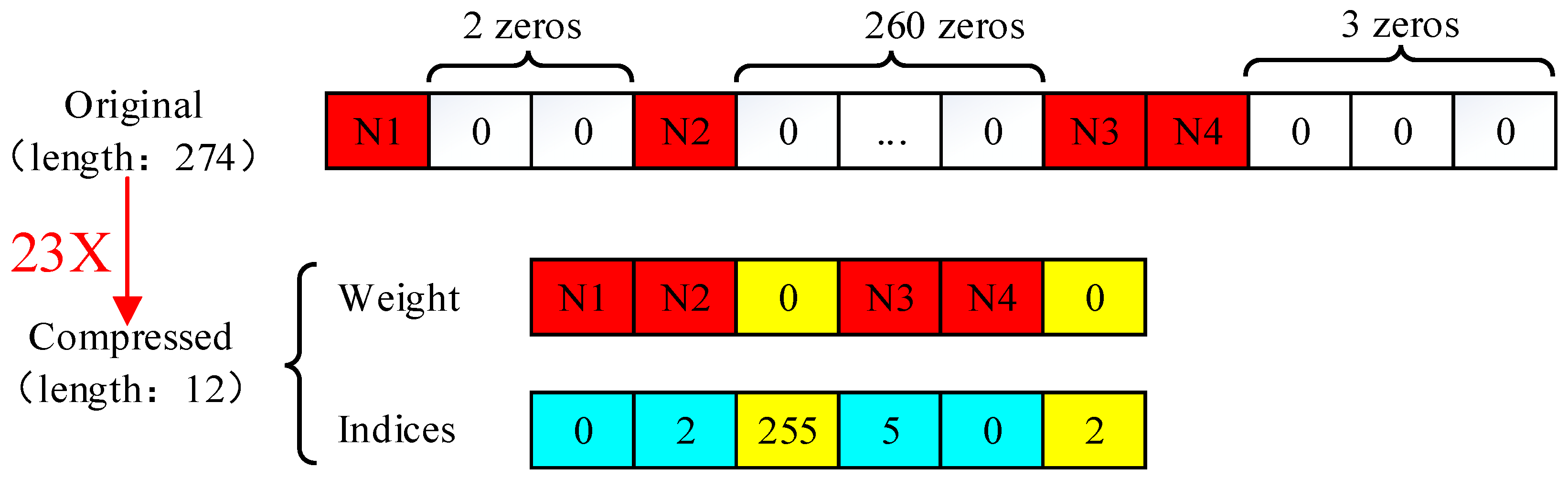
For the fully connected layer, the input was just a feature vector. After pruning and quantization, the feature vector was converted into a sparse vector. We proposed a straightforward approach to store these sparse vectors, only storing two arrays 2a + 2 numbers in total, where a is the number of non-zero elements. The relative index represents the number of zeros between the current non-zero weight and the previous one. When the relative index was larger than the bound, we insert a zero value as shown in
Figure 7. Another point to be noted is that when the last value of the original sparse vector was zero, an extra zero value was inserted into the weight array.
The final result of our model compression is shown in
Table 5, and we achieved 27× and 28× compressibility, respectively, compared with Han’s 27× for the original AlexNet. It should be noted that we only compared the benefits of pruning and quantification, without taking Huffman coding into consideration. For pruning, our improved reserve-pruning and peak-pruning techniques retained less non-zero weight. Although Han quantifies the weights of the CONV layer with 8 bits and the FC layer with 5 bits to achieve a smaller size, it is inefficient for 5 bit hardware computing. Another advantage of our method is that it does not need to store the codebook and its index, reducing additional storage and computation. We also obtained 34× compressibility for LeNet-5 on the MNIST dataset [
25]. The smaller the CNN model is, the less storage will be consumed, leading to less amount of calculations and higher inference speeds.
4. Hardware Implementation
The optimized pruning and quantization, though significantly reducing the memory footprint on FPGA, brings in some new challenges difficult for conventional FPGA-based accelerators to overcome. Firstly, irregular computation is introduced by model compression. After pruning, original dense computation becomes sparse computation. After quantization, the weights are stored with fewer bits. Secondly, load imbalance introduced by sparsity will reduce anticipative hardware efficiency. Based on the above findings and conclusions, we first customized decoding circuits to recover the original sparse weight matrix on FPGA. Considering the FPGA is especially friendly for byte-aligned data, weights and indices were stored with 8-bits according to the CCOO format. Moreover, by setting constraints during pruning, the overall number of non-zero weights distributed to each processing element (PE) unit was approximately equal to ensure sufficient parallelism and load balance of the FPGA. In addition, different from the algorithm of the CNN, pooling layers were placed between the convolutional layers and non-linear activation function ReLU to reduce the resource consumption and improve the inference speed.
4.1. Overall Architecture
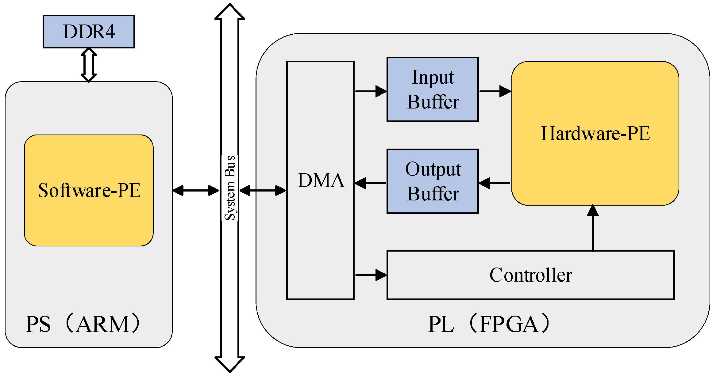
Figure 8 schematizes an overview of our implementation on Xilinx Zynq UltraScale + MPSOC XCZU7EV, which integrates a quad-core ARM Cortex-A53 processing system (PS) and FPGA programmable logic (PL). The XCZU7EV has 16 nm manufacturing technology and has abundant Ultra RAMs that alleviate the demand for the buffering and storage of insufficient SRAM resources on an FPGA chip. The external memory DDR4 stores compressed model parameters and input image.
The ARM realizes data transmission of instructions and convolutional results between the FPGA and the software-PE, which accomplishes the fully connected layers and softmax function. The FPGA consists of direct memory access (DMA), controller, input buffer, output buffer, and hardware-PE. The hardware-PE takes charge of convolutional layers, pooling layers, and non-linear functions. On-chip buffers, including the input buffer and output buffer, prepare data to be computed by hardware-PE and store the result. The controller analyzes the instructions from ARM and harmonizes modules according to FPGA resources, configuring the depth of input buffer and output buffer and the number of output feature maps in parallel.
Not all calculations are offloaded to the FPGA. One reason is that the parameters of the fully connected layer are relatively large, and the calculation is not intensive enough. The calculation unit of the FPGA needs large DDR bandwidth for maximum computational performance. The other is that the actual use of the number of categories is uncertain, with software implementation of the fully connected layer and softmax is conducive to modify.
4.2. Hardware-PE Architecture
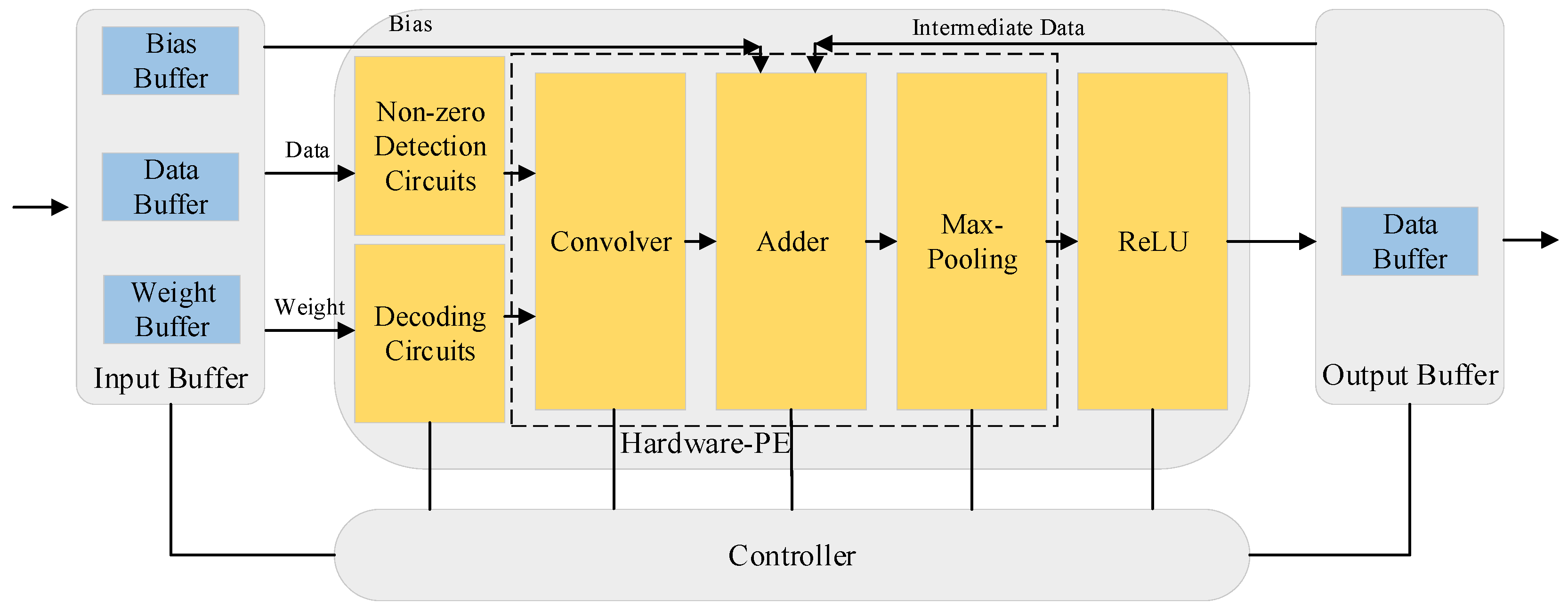
The hardware-PE takes charge of non-zero detection circuits, decoding circuits, convolutional layers, pooling layers, and the non-linear function ReLU.
Figure 9 describes the detailed hardware-PE architecture and other relative modules.
- (1)
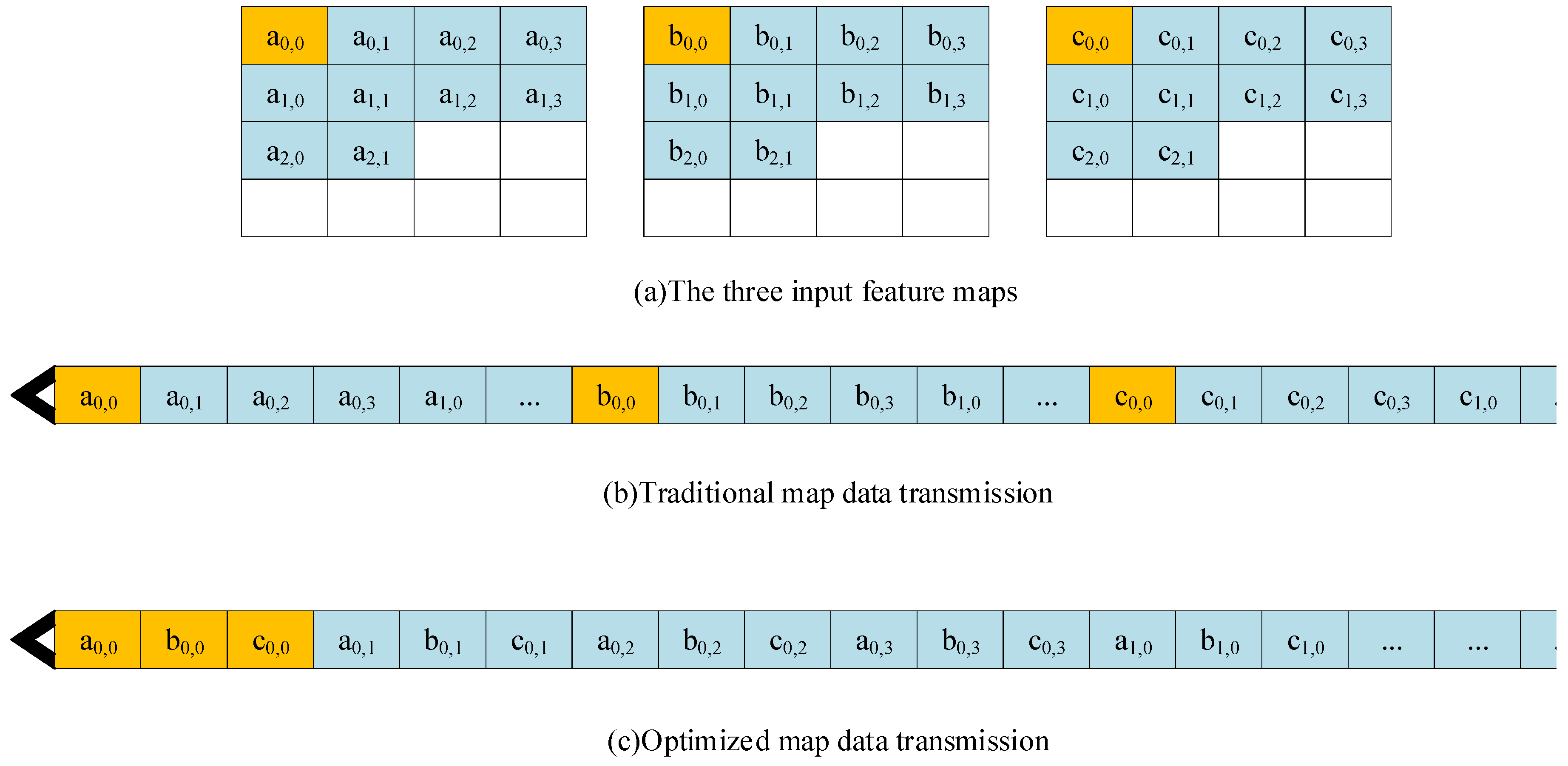
The data transmission form was optimized. In previous research, the transmission of the feature maps was performed by regarding each graph as a unit [
26]. As shown in
Figure 10, it was assumed that the input of a layer of the network was three feature maps, which was orderly stored in memory. The traditional form of data transmission, which reads out the first image line by line and then the second and third images. However, the output of the calculation results starts when all the data have been input to the calculation module, which leads to a large data output delay and a waste of computing resources. Therefore, we intended to optimize the transmission of map data. We performed the transmission in the unit of pixels, which transmits the first pixel of each map at first, and then the second pixel of each map. This optimization allows the module to calculate and output some of the results during the data transmission. Consequently, the output delay decreased and the waste of computing resources significantly reduced.
- (2)
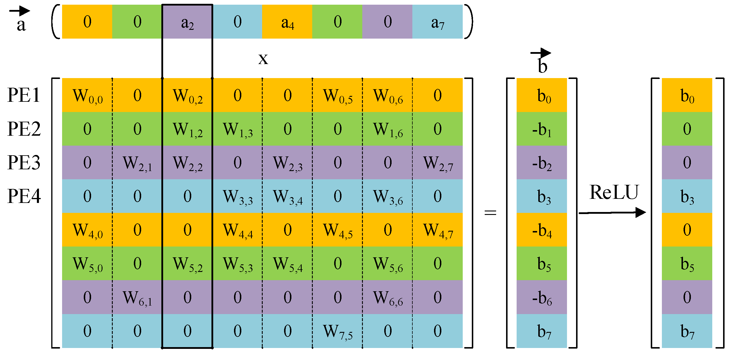
Non-zero detection circuits were used to hierarchically broadcast the non-zero input data to each PE according to the advantage of the input activation sparsity, as shown in
Figure 11. Multiplication occurred only when the input activation was a non-zero value, which greatly reduced computing resources.
- (1)
Decoding circuits were customized to recover the original sparse weight matrix according to the CCOO format of sparse non-zero weights and its indices. Compared with Han’s method, our decoding circuits did not require complex logic designs and extra calculations benefitting from the efficient storage approach we proposed in model compression.
- (2)
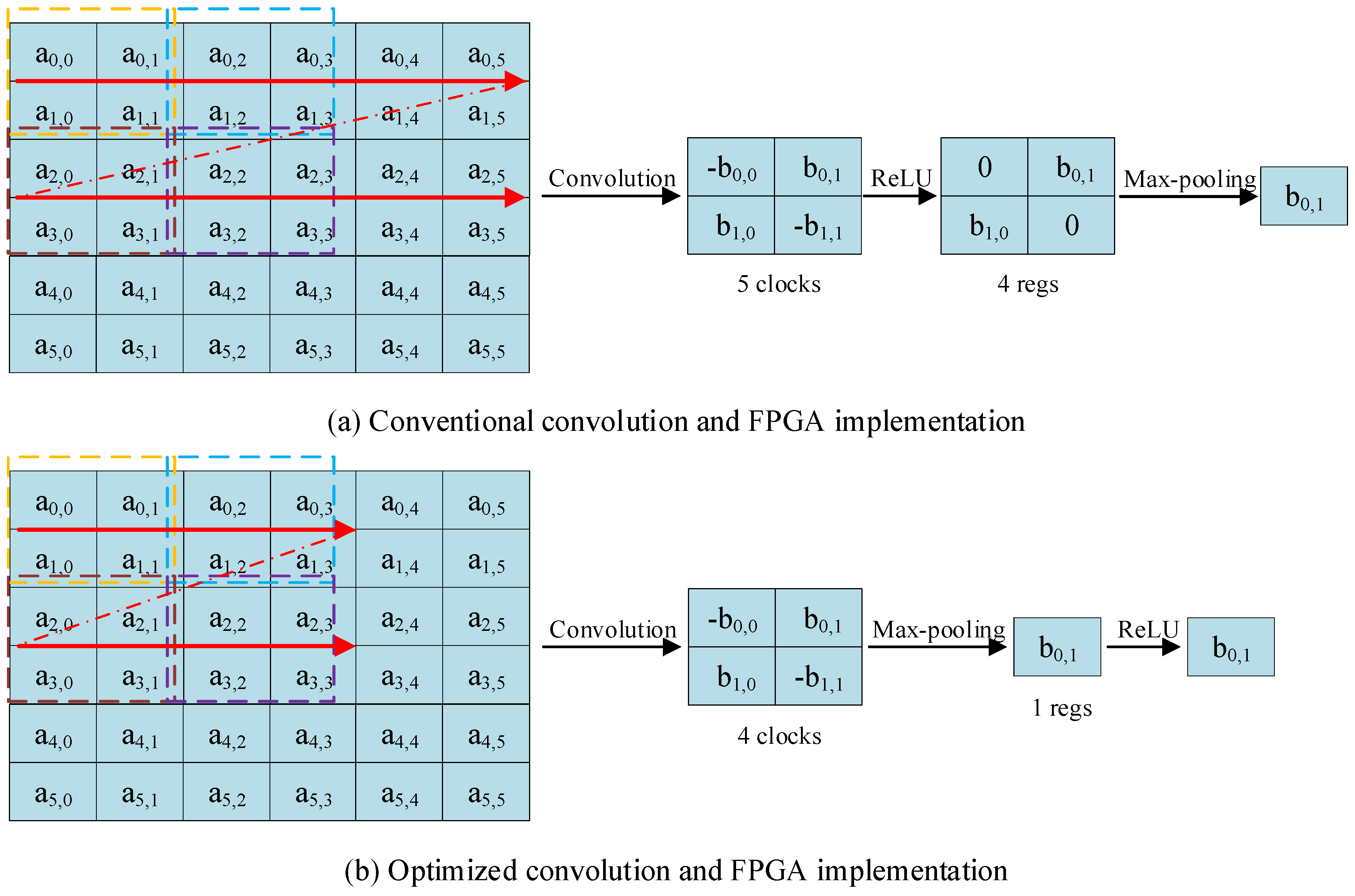
The convolver accomplished a window convolution operation, which was essentially multiplication. As illustrated in
Figure 12, the kernel size was 2 × 2, and the traditional window convolution was slided by row. When we placed pooling layers between the convolutional layers and ReLU, the window convolution was slided according to the size of window pooling, reducing the clock cycles and memory occupation of temporarily unused results. Another advantage was that this pipelining decreases the data cache by a factor of 4 after convolution, without affecting the final result.
- (1)
The adder sums all results from the convolver and bias from the input buffer or intermediate data from the output buffer if needed.
- (2)
Max-pooling applies a 2 × 2 window to the input feature map, and outputs the maximum among them.
- (3)
ReLU is a non-linear operator especially suitable for hardware implementation.
5. Performance Analysis
In order to verify the performance of the proposed FPGA accelerator, the design was implemented with a Xilinx SDx 2018.2, which accepts the C/C++ code as input and outputs the optimized CNN hardware implementation on FPGAs. Convolutional and max-pooling functions were implemented as hardware functions in SDx respectively, exporting the register-transfer level (RTL) as the Vivado IP core. Finally, a complete synthesized and implemented Vivado project was achieved.
We implemented the compressed AlexNet network inference on the Xilinx ZCU104 evaluation board. The XCZU7EV on the board has abundant resources, such as look-up table (LUT), look-up table RAM (LUTRAM), flip-flop (FF), block RAM (BRAM), Ultra RAM (URAM), digital signal processing (DSP) and global buffer (BUFG). The proposed FPGA implementations of the CNN were operating at 300 MHz. According to the device utilization summary given by the Vivado design suite, the resource utilization of the main hardware resources for the compressed AlexNet is shown in
Table 6. The reason why RAM and DSP take a relatively large percentage is that the weight parameters need to be stored on-chip and multiplication and accumulation (MAC) is accomplished by DSP48E block.
Implementations of the AlexNet inference on CPU, GPU, and our accelerator were compared, as shown in
Table 7. The overall performances, especially the CONV layers, are as follows. In our design, FPGA mainly takes charge of the convolutional layers and the pooling layers while the ARM implements fully connected layers and the softmax function. The CPU platform was Intel i7-6700 CPU @ 3.40 GHz with 32 GB DDR4 DRAM. The GPU platform was NVIDIA GTX 1080 Ti GPU, possessing 3584 compute unified device architecture (CUDA) cores with 11 GB graphics double data rate (GDDR) 5 352-bit memory. Compared to the CPU and the GPU, our accelerator achieved a 182.3× and 1.1× improvement on the CONV layers of AlexNet in terms of latency and throughput, respectively. The thermal design power (TDP) values of the CPU and GPU were 65 W and 250 W, separately. The total power of our accelerator was only 17.67 W according to the power report by the Vivado design suite. It can be seen from
Table 7 that our accelerator achieved the best energy efficiency among all the platforms. Contrasted to the CPU and the GPU, our accelerator achieved an 822.0× and 15.8× improvement on CONV layers of AlexNet in terms of energy efficiency, respectively.
The performance comparison between our accelerator and other FPGA-based counterparts is shown in
Table 8. Our accelerator achieved an outstanding performance of 290.40 GOP/s and an energy efficiency of 16.44 GOP/s/W for CONV layers. Since not all calculations are offloaded to the FPGA in our accelerator, the overall performance of our accelerator is slightly inferior to previous approaches. Besides, the working frequency is 300 MHz for the DSP48E block, which greatly improves the computational performance.
6. Conclusions
In this paper, we proposed an improved compression strategy and an efficient FPGA-based accelerator for the compressed CNN. We first compressed a trained convolutional neural network model sufficiently, including reverse-pruning and peak-pruning within fewer weights and a linear quantization strategy for lower precision. Then, we developed efficient storage methods for the convolutional layer and the fully connected layer to decrease the occupancy of the overhead cache, respectively. Taking the AlexNet as an example, our work achieved 27× (reverse-pruning) and 28× (peak-pruning) compressibility, respectively. We also obtained 34× compressibility for LeNet-5 on the MNIST dataset. An FPGA-based accelerator was realized to evaluate the performance of the compressed CNN. The system implemented on a Xilinx Zynq ZCU104 board achieved a frame rate of 9.73 fps. Compared with the CPU and GPU platforms, our accelerator achieved 182.3× and 1.1× improvements in latency and throughput, respectively, on the CONV layers of AlexNet, with 822.0× and 15.8× improvement for energy efficiency, separately. Evaluation results verified the effectiveness of the proposed compression strategy for an FPGA-based CNN accelerator, and this provides a reference for other neural network applications, including CNNs, LSTMs, and RNNs.


