Review

A State-of-the-Art Survey on Deep Learning Theory and Architectures

1
Department of Electrical and Computer Engineering, University of Dayton, Dayton, OH 45469, USA
2
Department of Earth and Atmospheric Sciences, Saint Louis University, Saint Louis, MO 63108, USA
3
Comcast Labs, Washington, DC 20005, USA
4
Lawrence Livermore National Laboratory (LLNL), Livermore, CA 94550, USA
*
Author to whom correspondence should be addressed.
Electronics 2019, 8(3), 292; https://doi.org/10.3390/electronics8030292
Submission received: 17 January 2019 / Accepted: 31 January 2019 / Published: 5 March 2019
(This article belongs to the Section Computer Science & Engineering)

Abstract

:
In recent years, deep learning has garnered tremendous success in a variety of application domains. This new field of machine learning has been growing rapidly and has been applied to most traditional application domains, as well as some new areas that present more opportunities. Different methods have been proposed based on different categories of learning, including supervised, semi-supervised, and un-supervised learning. Experimental results show state-of-the-art performance using deep learning when compared to traditional machine learning approaches in the fields of image processing, computer vision, speech recognition, machine translation, art, medical imaging, medical information processing, robotics and control, bioinformatics, natural language processing, cybersecurity, and many others. This survey presents a brief survey on the advances that have occurred in the area of Deep Learning (DL), starting with the Deep Neural Network (DNN). The survey goes on to cover Convolutional Neural Network (CNN), Recurrent Neural Network (RNN), including Long Short-Term Memory (LSTM) and Gated Recurrent Units (GRU), Auto-Encoder (AE), Deep Belief Network (DBN), Generative Adversarial Network (GAN), and Deep Reinforcement Learning (DRL). Additionally, we have discussed recent developments, such as advanced variant DL techniques based on these DL approaches. This work considers most of the papers published after 2012 from when the history of deep learning began. Furthermore, DL approaches that have been explored and evaluated in different application domains are also included in this survey. We also included recently developed frameworks, SDKs, and benchmark datasets that are used for implementing and evaluating deep learning approaches. There are some surveys that have been published on DL using neural networks and a survey on Reinforcement Learning (RL). However, those papers have not discussed individual advanced techniques for training large-scale deep learning models and the recently developed method of generative models.

1. Introduction

Since the 1950s, a small subset of Artificial Intelligence (AI), often called Machine Learning (ML), has revolutionized several fields in the last few decades. Neural Networks (NN) is a subfield of ML, and it was this subfield that spawned Deep Learning (DL). Since its inception DL has been creating ever larger disruptions, showing outstanding success in almost every application domain. Figure 1 shows the taxonomy of AI. DL which uses either deep architectures of learning or hierarchical learning approaches), is a class of ML developed largely from 2006 onward. Learning is a procedure consisting of estimating the model parameters so that the learned model (algorithm) can perform a specific task. For example, in Artificial Neural Networks (ANN), the parameters are the weight matrices. DL, on the other hand, consists of several layers in between the input and output layer which allows for many stages of non-linear information processing units with hierarchical architectures to be present that are exploited for feature learning and pattern classification [1,2]. Learning methods based on representations of data can also be defined as representation learning [3]. Recent literature states that DL based representation learning involves a hierarchy of features or concepts, where the high-level concepts can be defined from the low-level ones and low-level concepts can be defined from high-level ones. In some articles, DL has been described as a universal learning approach that is able to solve almost all kinds of problems in different application domains. In other words, DL is not task specific [4].

1.1. Type of Deep Learning Approaches

Deep learning approaches can be categorized as follows: Supervised, semi-supervised or partially supervised, and unsupervised. In addition, there is another category of learning approach called Reinforcement Learning (RL) or Deep RL (DRL) which are often discussed under the scope of semi-supervised or sometimes under unsupervised learning approaches. Figure 2 shows the pictorial diagram.

1.1.1. Deep Supervised Learning

Supervised learning is a learning technique that uses labeled data. In the case of supervised DL approaches, the environment has a set of inputs and corresponding outputs ( x t , y t ) ~ ρ . For example, if for input xt, the intelligent agent predicts y ^ t = f ( x t ) , the agent will receive a loss value l ( y t , y ^ t ) . The agent will then iteratively modify the network parameters for a better approximation of the desired outputs. After successful training, the agent will be able to get the correct answers to questions from the environment. There are different supervised learning approaches for deep leaning, including Deep Neural Networks (DNN), Convolutional Neural Networks (CNN), Recurrent Neural Networks (RNN), including Long Short Term Memory (LSTM), and Gated Recurrent Units (GRU). These networks will be described in details in the respective sections.

1.1.2. Deep Semi-supervised Learning

Semi-supervised learning is learning that occurs based on partially labeled datasets. In some cases, DRL and Generative Adversarial Networks (GAN) are used as semi-supervised learning techniques. GAN is discussed in Section 7. Section 8 surveys DRL approaches. Additionally, RNN, including LSTM and GRU, are used for semi-supervised learning as well.

1.1.3. Deep Unsupervised Learning

Unsupervised learning systems are ones that can without the presence of data labels. In this case, the agent learns the internal representation or important features to discover unknown relationships or structure within the input data. Often clustering, dimensionality reduction, and generative techniques are considered as unsupervised learning approaches. There are several members of the deep learning family that are good at clustering and non-linear dimensionality reduction, including Auto-Encoders (AE), Restricted Boltzmann Machines (RBM), and the recently developed GAN. In addition, RNNs, such as LSTM and RL, are also used for unsupervised learning in many application domains. Section 6 and Section 7 discuss RNNs and LSTMs in detail.

1.1.4. Deep Reinforcement Learning (RL)

Deep Reinforcement Learning is a learning technique for use in unknown environments. DRL began in 2013 with Google Deep Mind [5,6]. From then on, several advanced methods have been proposed based on RL. Here is an example of RL: If environment samples inputs: x t ~ ρ , agent predict: y ^ t = f ( x t ) , agent receive cost: c t ~ P ( c t | x t , y ^ t ) where P is an unknown probability distribution, the environment asks an agent a question, and gives a noisy score as the answer. Sometimes this approach is called semi-supervised learning as well. There are many semi-supervised and un-supervised techniques that have been implemented based on this concept (in Section 8). In RL, we do not have a straight forward loss function, thus making learning harder compared to traditional supervised approaches. The fundamental differences between RL and supervised learning are: First, you do not have full access to the function you are trying to optimize; you must query them through interaction, and second, you are interacting with a state-based environment: Input x t depends on previous actions.
Depending upon the problem scope or space, one can decide which type of RL needs to be applied for solving a task. If the problem has a lot of parameters to be optimized, DRL is the best way to go. If the problem has fewer parameters for optimization, a derivation free RL approach is good. An example of this is annealing, cross entropy methods, and SPSA.

1.2. Feature Learning

A key difference between traditional ML and DL is in how features are extracted. Traditional ML approaches use handcrafted engineering features by applying several feature extraction algorithms, and then apply the learning algorithms. Additionally, other boosting approaches are often used where several learning algorithms are applied to the features of a single task or dataset and a decision is made according to the multiple outcomes from the different algorithms.
On the other hand, in the case of DL, the features are learned automatically and are represented hierarchically in multiple levels. This is the strong point of DL against traditional machine learning approaches. Table 1 shows the different feature-based learning approaches with different learning steps.

1.3. Why and When to apply DL

DL is employed in several situations where machine intelligence would be useful (see Figure 3):
  • Absence of a human expert (navigation on Mars)
  • Humans are unable to explain their expertise (speech recognition, vision, and language understanding)
  • The solution to the problem changes over time (tracking, weather prediction, preference, stock, price prediction)
  • Solutions need to be adapted to the particular cases (biometrics, personalization).
  • The problem size is too vast for our limited reasoning capabilities (calculation webpage ranks, matching ads to Facebook, sentiment analysis).
At present, DL is being applied in almost all areas. As a result, this approach is often called a universal learning approach.

1.4. The State-of-the-art Performance of DL

There are some outstanding successes in the fields of computer vision and speech recognition as discussed below:
(a). Image classification on ImageNet dataset. One of the large-scale problems is named Large Scale Visual Recognition Challenge (LSVRC). CNN and its variants as one of the DL branches showed state-of-the-art accuracy on the ImageNet task [7,8,9,10,11,12]. The following graph shows the success story of DL techniques overtime on ImageNet-2012 challenge. Figure 3 shows that ResNet-152 has achieved 3.57% error rate which outperformed human accuracy.
(b). Automatic speech recognition. The initial success in the field of speech recognition on the popular TIMIT dataset (common data set are generally used for evaluation) was with small-scale recognition tasks [24]. The TIMIT Acoustic-Phonetic continuous speech Corpus contains 630 speakers from eight major dialects of American English, where each speaker reads 10 sentences. Figure 4 summarizes the error rates, including these early results and is measured as a percent phone error rate (PER) over the last 20 years. The bar graph clearly shows that the recently developed DL approaches (top of the graph) perform better compared to any other previous machine learning approaches on the TIMIT dataset.
Some example applications are shown in Figure 5 and Figure 6.

1.5. Why DL?

1.5.1. Universal Learning Approach

The DL approach is sometimes called universal learning because it can be applied to almost any application domain.

1.5.2. Robust

Deep learning approaches do not require the precisely designed feature. Instead, optimal features are automatically learned for the task at hand. As a result, the robustness to natural variations of the input data is achieved.

1.5.3. Generalization

The same DL approach can be used in different applications or with different data types. This approach is often called transfer learning. In addition, this approach is helpful where the problem does not have sufficient available data. There are a number of literatures that have discussed this concept (See Section 4).

1.5.4. Scalability

The DL approach is highly scalable. Microsoft invented a deep network known as ResNet [11]. This network contains 1202 layers and is often implemented at a supercomputing scale. There is a big initiative at Lawrence Livermore National Laboratory (LLNL) in developing frameworks for networks like this, which can implement thousands of nodes [24].

1.6. Challenges of DL

There are several challenges for DL:
  • Big data analytics using DL
  • Scalability of DL approaches
  • Ability to generate data which is important where data is not available for learning the system (especially for computer vision task, such as inverse graphics).
  • Energy efficient techniques for special purpose devices, including mobile intelligence, FPGAs, and so on.
  • Multi-task and transfer learning or multi-module learning. This means learning from different domains or with different models together.
  • Dealing with causality in learning.
Most of the above-mentioned challenges have already been considered by the DL community. Firstly, for the big data analytics challenge, there is a good survey that was conducted in 2014 [30]. In this paper, the authors explained details on how DL can deal with different criteria, including volume, velocity, variety, and veracity of the big data problem. The authors also showed different advantages of DL approaches when dealing with big data problems [31,32]. Figure 7 clearly demonstrates that the performance of traditional ML approaches shows better performance for lesser amounts of input data. As the amount of data increases beyond a certain number, the performance of traditional machine learning approaches becomes steady, whereas DL approaches increase with respect to the increment of the amount of data.
Secondly, in most of the cases for solving large-scale problems, the solution is being implemented on High-Performance Computing (HPC) system (super-computing, cluster, sometimes considered cloud computing) which offers immense potential for data-intensive business computing. As data explodes in velocity, variety, veracity, and volume, it is getting increasingly difficult to scale compute performance using enterprise-class servers and storage in step with the increase. Most of the articles considered all the demands and suggested efficient HPC with heterogeneous computing systems. In one example, Lawrence Livermore National Laboratory (LLNL) has developed a framework which is called Livermore Big Artificial Neural Networks (LBANN) for large-scale implementation (in super-computing scale) for DL which clearly supplants the issue of scalability of DL [24].
Thirdly, generative models are another challenge for deep learning. One example is the GAN, which is an outstanding approach for data generation for any task which can generate data with the same distribution [33]. Fourthly, multi-task and transfer learning which we have discussed in Section 7. Fourthly, there is a lot of research that has been conducted on energy efficient deep learning approaches with respect to network architectures and hardwires. Section 10 discusses this issue.
Can we make any uniform model that can solve multiple tasks in different application domains? As far as the multi-model system is concerned, one article from Google titled One Model To Learn Them All [34] is a good example. This approach can learn from different application domains, including ImageNet, multiple translation tasks, Image captioning (MS-COCO dataset), speech recognition corpus and English parsing task. We will be discussing most of the challenges and respective solutions through this survey. There are some other multi-task techniques that have been proposed in the last few years [35,36,37].
Finally, a learning system with causality has been presented, which is a graphical model that defines how one may infer a causal model from data. Recently a DL based approach has been proposed for solving this type of problem [38]. However, there are other many challenging issues have been solved in the last few years which were not possible to solve efficiently before this revolution. For example, image or video captioning [39], style transferring from one domain to another domain using GAN [40], text to image synthesis [41], and many more [42].
There are some surveys that have been conducted recently in the DL field [43,44,45,46]. These papers survey on DL and its revolution, but they did not address the recently developed generative model called GAN [33]. In addition, they discuss little RL and did not cover recent trends of DRL approaches [1,44]. In most of the cases, the surveys that have been conducted are on different DL approaches individually. There is a good survey which is based on Reinforcement Learning approaches [46,47]. Another survey exists on transfer learning [48]. One survey has been conducted on neural network hardware [49]. However, the main objective of this work is to provide an overall idea on deep learning and its related fields, including deep supervised (e.g., DNN, CNN, and RNN), unsupervised (e.g., AE, RBM, GAN) (sometimes GAN also used for semi-supervised learning tasks) and DRL. In some cases, DRL is considered to be a semi-supervised or an unsupervised approach. In addition, we have considered the recently developing trends in this field and applications which are developed based on these techniques. Furthermore, we have included the framework and benchmark datasets which are often used for evaluating deep learning techniques. Moreover, the name of the conferences and journals are also included which are considered by this community for publishing their research articles.
The rest of the paper has been organized in the following ways: The detailed surveys of DNNs are discussed in Section 2, Section 3 discusses on CNN. Section 4 describes different advanced techniques for efficient training of DL approaches. Section 5 discusses RNNs. AEs and RBMs are discussed in Section 6. GANs with applications are discussed in Section 7. RL is presented in Section 8. Section 9 explains transfer learning. Section 10 presents energy efficient approaches and hardwires for DL. Section 11 discusses deep learning frameworks and standard development kits (SDK). The benchmarks for different application domains with web links are given in Section 12. The conclusions are made in Section 13.

2. Deep Neural Network

2.1. The History of DNN

A brief history of neural networks highlighting key events is, as shown in Figure 8. Computational neurobiology has conducted significant research on constructing computational models of artificial neurons. Artificial neurons, which try to mimic the behavior of the human brain, are the fundamental component for building ANNs. The basic computational element (neuron) is called a node (or unit) which receives inputs from external sources and has some internal parameters (including weights and biases that are learned during training) which produce outputs. This unit is called a perceptron. The fundamental of ANN is discussed in References [1,3].
ANNs or general NNs consist of Multilayer Perceptron’s (MLP) which contain one or more hidden layers with multiple hidden units (neurons) in them. For details on MLP, please see in References [1,3,53]

2.2. Gradient Descent

The gradient descent approach is a first-order optimization algorithm which is used for finding the local minima of an objective function. This has been used for training ANNs in the last couple of decades successfully [1,53].

2.3. Stochastic Gradient Descent (SGD)

Since a long training time is the main drawback for the traditional gradient descent approach, the SGD approach is used for training Deep Neural Networks (DNN) [1,58].

2.4. Back-Propagation (BP)

DNN is trained with the popular Back-Propagation (BP) algorithm with SGD [47,53]. In the case of MLPs, we can easily represent NN models using computation graphs which are directive acyclic graphs. For that representation of DL, we can use the chain-rule to efficiently calculate the gradient from the top to the bottom layers with BP, as shown in References [53,59,60,61,62,63].

2.5. Momentum

Momentum is a method which helps to accelerate the training process with the SGD approach. The main idea behind it is to use the moving average of the gradient instead of using only the current real value of the gradient. We can express this with the following equation mathematically:
v t = γ   v t 1 η     ( θ t 1 ) ,
θ t = θ t 1 +   v t ,
here γ is the momentum and η is the learning rate for the tth round of training. Other popular approaches have been introduced during the last few years which are explained in Section 9 under the scope of optimization approaches. The main advantage of using momentum during training is to prevent the network from getting stuck in local minimum. The values of momentum are γ ∈ (0,1]. It is noted that a higher momentum value overshoots its minimum, possibly making the network unstable. In general, γ is set to 0.5 until the initial learning stabilizes and is then increased to 0.9 or higher [60].

2.6. Learning Rate ( η )

The learning rate is an important component for training DNN. The learning rate is the step size considered during training which makes the training process faster. However, selecting the value of the learning rate is sensitive. For example: If you choose a larger value for η , the network may start diverging instead of converging. On the other hand, if you choose a smaller value for η , it will take more time for the network to converge. In addition, it may easily get stuck in local minima. The typical solution to this problem is to reduce the learning rate during training [64].
There are three common approaches used for reducing the learning rate during training: Constant, factored, and exponential decay. First, we can define a constant ζ which is applied to reduce the learning rate manually with a defined step function. Second, the learning rate can be adjusted during training with the following equation:
η t = η 0 β t ϵ ,
where η t is the tth round learning rate, η 0 is the initial learning rate, and β is the decay factor with a value between the range of ( 0 , 1 ) .
The step function format for exponential decay is:
η t = η 0 β t ϵ .
The common practice is to use a learning rate decay of β = 0.1 to reduce the learning rate by a factor of 10 at each stage.

2.7. Weight Decay

Weight decay is used for training deep learning models as an L2 regularization approach, which helps to prevent overfitting the network and model generalization. L2 regularization for ( θ , x ) can be defined as,
Ω = θ 2 ,
ε ^ ( ( θ , x ) , y ) = ε ( ( θ , x ) , y ) +   1 2 λ   Ω .
The gradient for the weight θ is:
1 2 λ Ω θ =   λ · θ .
General practice is to use the value λ = 0.0004 . A smaller λ will accelerate training.
Other necessary components for efficient training, including data preprocessing and augmentation, network initialization approaches, batch normalization, activation functions, regularization with dropout, and different optimization approaches (as discussed in Section 4).
In the last few decades, many efficient approaches have been proposed for better training of deep neural networks. Before 2006, attempts taken at training deep architectures failed: Training a deep supervised feed-forward neural network tended to yield worse results (both in training and in test error) than shallow ones (with 1 or 2 hidden layers). Hinton’s revolutionary work on DBNs spearheaded a change in this in 2006 [56,59].
Due to their composition, many layers of DNNs are more capable of representing highly varying nonlinear functions compared to shallow learning approaches [62,63,64,65]. Moreover, DNNs are more efficient for learning because of the combination of feature extraction and classification layers. The following sections discuss in detail about different DL approaches with necessary components.

3. Convolutional Neural Network (CNN)

3.1. CNN Overview

This network structure was first proposed by Fukushima in 1988 [54]. It was not widely used, however, due to limits of computation hardware for training the network. In the 1990s, LeCun et al. [55] applied a gradient-based learning algorithm to CNNs and obtained successful results for the handwritten digit classification problem. After that, researchers further improved CNNs and reported state-of-the-art results in many recognition tasks. CNNs have several advantages over DNNs, including being more like the human visual processing system, being highly optimized in the structure for processing 2D and 3D images, and being effective at learning and extracting abstractions of 2D features. The max pooling layer of CNNs is effective in absorbing shape variations. Moreover, composed of sparse connections with tied weights, CNNs have significantly fewer parameters than a fully connected network of similar size. Most of all, CNNs are trained with the gradient-based learning algorithm and suffer less from the diminishing gradient problem. Given that the gradient-based algorithm trains the whole network to minimize an error criterion directly, CNNs can produce highly optimized weights.
Figure 9 shows the overall architecture of CNNs consists of two main parts: Feature extractors and a classifier. In the feature extraction layers, each layer of the network receives the output from its immediate previous layer as its input and passes its output as the input to the next layer. The CNN architecture consists of a combination of three types of layers: Convolution, max-pooling, and classification. There are two types of layers in the low and middle-level of the network: Convolutional layers and max-pooling layers. The even numbered layers are for convolutions and the odd-numbered layers are for max-pooling operations. The output nodes of the convolution and max-pooling layers are grouped into a 2D plane called feature mapping. Each plane of a layer is usually derived from the combination of one or more planes of previous layers. The nodes of a plane are connected to a small region of each connected planes of the previous layer. Each node of the convolution layer extracts the features from the input images by convolution operations on the input nodes.
Higher-level features are derived from features propagated from lower level layers. As the features propagate to the highest layer or level, the dimensions of features are reduced depending on the size of the kernel for the convolutional and max-pooling operations respectively. However, the number of feature maps usually increased for representing better features of the input images for ensuring classification accuracy. The output of the last layer of the CNN is used as the input to a fully connected network which is called classification layer. Feed-forward neural networks have been used as the classification layer as they have better performance [56,64]. In the classification layer, the extracted features are taken as inputs with respect to the dimension of the weight matrix of the final neural network. However, the fully connected layers are expensive in terms of network or learning parameters. Nowadays, there are several new techniques, including average pooling and global average pooling that is used as an alternative of fully-connected networks. The score of the respective class is calculated in the top classification layer using a soft-max layer. Based on the highest score, the classifier gives output for the corresponding classes. Mathematical details on different layers of CNNs are discussed in the following section.

3.1.1. Convolutional Layer

In this layer, feature maps from previous layers are convolved with learnable kernels. The output of the kernels goes through a linear or non-linear activation function, such as sigmoid, hyperbolic tangent, Softmax, rectified linear, and identity functions) to form the output feature maps. Each of the output feature maps can be combined with more than one input feature map. In general, we have that
x j l = f ( i ϵ M j x i l 1   k i j l +   b j l ) ,
where x j l is the output of the current layer, x i l 1 is the previous layer output, k i j l is the kernel for the present layer, and b j l are the biases for the current layer. M j represents a selection of input maps. For each output map, an additive bias b is given. However, the input maps will be convolved with distinct kernels to generate the corresponding output maps. The output maps finally go through a linear or non-linear activation function (such as sigmoid, hyperbolic tangent, Softmax, rectified linear, or identity functions).

3.1.2. Sub-sampling Layer

The subsampling layer performs the down sampled operation on the input maps. This is commonly known as the pooling layer. In this layer, the number of input and output feature maps does not change. For example, if there are N input maps, then there will be exactly N output maps. Due to the down sampling operation, the size of each dimension of the output maps will be reduced, depending on the size of the down sampling mask. For example, if a 2 × 2 down sampling kernel is used, then each output dimension will be half of the corresponding input dimension for all the images. This operation can be formulated as
x j l = down ( x j l 1 ) ,
where down ( . ) represents a sub-sampling function. Two types of operations are mostly performed in this layer: Average pooling or max-pooling. In the case of the average pooling approach, the function usually sums up over N × N patches of the feature maps from the previous layer and selects the average value. On the other hand, in the case of max-pooling, the highest value is selected from the N × N patches of the feature maps. Therefore, the output map dimensions are reduced by n times. In some special cases, each output map is multiplied with a scalar. Some alternative sub-sampling layers have been proposed, such as fractional max-pooling layer and sub-sampling with convolution. These are explained in Section 4.6.

3.1.3. Classification Layer

This is the fully connected layer which computes the score of each class from the extracted features from a convolutional layer in the preceding steps. The final layer feature maps are represented as vectors with scalar values which are passed to the fully connected layers. The fully connected feed-forward neural layers are used as a soft-max classification layer. There are no strict rules on the number of layers which are incorporated in the network model. However, in most cases, two to four layers have been observed in different architectures, including LeNet [55], AlexNet [7], and VGG Net [9]. As the fully connected layers are expensive in terms of computation, alternative approaches have been proposed during the last few years. These include the global average pooling layer and the average pooling layer which help to reduce the number of parameters in the network significantly.
In the backward propagation through the CNNs, the fully connected layer updates following the general approach of fully connected neural networks (FCNN). The filters of the convolutional layers are updated by performing the full convolutional operation on the feature maps between the convolutional layer and its immediate previous layer. Figure 10 shows the basic operations in the convolution and sub-sampling of an input image.

3.1.4. Network Parameters and Required Memory for CNN

The number of computational parameters is an important metric to measure the complexity of a deep learning model. The size of the output feature maps can be formulated as follows:
M = ( N F ) S   + 1 ,
where N refers to the dimensions of the input feature maps, F refers to the dimensions of the filters or the receptive field, M refers to the dimensions of output feature maps, and S stands for the stride length. Padding is typically applied during the convolution operations to ensure the input and output feature map have the same dimensions. The amount of padding depends on the size of the kernel. Equation (17) is used for determining the number of rows and columns for padding.
P = ( F 1 ) / 2 ,
here P is the amount of padding and F refers to the dimension of the kernels. Several criteria are considered for comparing the models. However, in most of the cases, the number of network parameters and the total amount of memory are considered. The number of parameters ( P a r m l ) of l t h layer is the calculated based on the following equation:
P a r m l = ( F × F × F M l 1 ) × F M l .
If bias is added with the weights, then the above equation can be written as follows:
  P a r m l = ( F × ( F + 1 ) ×   F M l 1 ) × F M l ,
here the total number of parameters of l t h lathe yer can be represented with P l , F M l is for the total number of output feature maps, and F M l 1 is the total number of input feature maps or channels. For example, let’s assume the l t h layer has F M l 1 = 32 input features maps, F M l = 64 output feature maps, and the filter size is F = 5 . In this case, the total number of parameters with a bias for this layer: P a r m l = ( 5 × 5 × 33 ) × 64 = 528,000 . Thus, the amount of memory ( M e m l ) needs for the operations of the l t h layer can be expressed as
M e m l = ( N l × N l × F M l   ) .

3.2. Popular CNN Architectures

In this section, several popular state-of-the-art CNN architectures will be examined. In general, most deep convolutional neural networks are made of a key set of basic layers, including the convolution layer, the sub-sampling layer, dense layers, and the soft-max layer. The architectures typically consist of stacks of several convolutional layers and max-pooling layers followed by a fully connected and SoftMax layers at the end. Some examples of such models are LeNet [55], AlexNet [7], VGG Net [9], NiN [66] and all convolutional (All Conv) [67]. Other alternatives and more efficient advanced architectures have been proposed, including DenseNet [68], FractalNet [69], GoogLeNet with Inception units [10,70,71], and Residual Networks [11]. The basic building components (convolution and pooling) are almost the same across these architectures. However, some topological differences are observed in the modern deep learning architectures. Of the many DCNN architectures, AlexNet [7], VGG [9], GoogLeNet [10,70,71], Dense CNN [68] and FractalNet [69] are generally considered the most popular architectures because of their state-of-the-art performance on different benchmarks for object recognition tasks. Among all of these structures, some of the architectures are designed especially for large-scale data analysis (such as GoogLeNet and ResNet), whereas the VGG network is considered a general architecture. Some of the architectures are dense in terms of connectivity, such as DenseNet [68]. Fractal Network is an alternative of ResNet model.

3.2.1. LeNet (1998)

Although LeNet was proposed in the 1990s, limited computation capability and memory capacity made the algorithm difficult to implement until about 2010 [55]. LeCun et al. [55], however, proposed CNNs with the back-propagation algorithm and experimented on handwritten digit dataset to achieve state-of-the-art accuracy. The proposed CNN architecture is well-known as LeNet-5 [55]. The basic configuration of LeNet-5 is as follows (see Figure 11): Two convolutions (conv) layers, two sub-sampling layers, two fully connected layers, and an output layer with the Gaussian connection. The total number of weights and Multiply and Accumulates (MACs) are 431 k and 2.3 M, respectively.
As computational hardware started improving in capability, CNNs stated becoming popular as an effective learning approach in the computer vision and machine learning communities.

3.2.2. AlexNet (2012)

In 2012, Alex Krizhevesky and others proposed a deeper and wider CNN model compared to LeNet and won the most difficult ImageNet challenge for visual object recognition called the ImageNet Large Scale Visual Recognition Challenge (ILSVRC) in 2012 [7]. AlexNet achieved state-of-the-art recognition accuracy against all the traditional machine learning and computer vision approaches. It was a significant breakthrough in the field of machine learning and computer vision for visual recognition and classification tasks and is the point in history where interest in deep learning increased rapidly.
The architecture of AlexNet is shown in Figure 12. The first convolutional layer performs convolution and max-pooling with Local Response Normalization (LRN) where 96 different receptive filters are used that are 11 × 11 in size. The max pooling operations are performed with 3 × 3 filters with a stride size of 2. The same operations are performed in the second layer with 5 × 5 filters. 3 × 3 filters are used in the third, fourth, and fifth convolutional layers with 384, 384, and 296 feature maps respectively. Two fully connected (FC) layers are used with dropout followed by a Softmax layer at the end. Two networks with similar structure and the same number of feature maps are trained in parallel for this model. Two new concepts, Local Response Normalization (LRN) and dropout, are introduced in this network. LRN can be applied in two different ways: First applying on single channel or feature maps, where an N × N patch is selected from the same feature map and normalized based on the neighborhood values. Second, LRN can be applied across the channels or feature maps (neighborhood along the third dimension but a single pixel or location).
AlexNet has three convolution layers and two fully connected layers. When processing the ImageNet dataset, the total number of parameters for AlexNet can be calculated as follows for the first layer: Input samples are 224 × 224 × 3, filters (kernels or masks) or a receptive field that has a size 11, the stride is 4, and the output of the first convolution layer is 55 × 55 × 96. According to the equations in Section 3.1.4, we can calculate that this first layer has 290,400 (55 × 55 × 96) neurons and 364 (11 ×11 × 3 = 363 + 1 bias) weights. The parameters for the first convolution layer are 290,400 × 364 = 105,705,600. Table 2 shows the number of parameters for each layer in millions. The total number of weights and MACs for the whole network are 61M and 724M, respectively.

3.2.3. ZFNet / Clarifai (2013)

In 2013, Matthew Zeiler and Rob Fergue won the 2013 ILSVRC with a CNN architecture which was an extension of AlexNet. The network was called ZFNet [8], after the authors’ names. As CNNs are expensive computationally, an optimum use of parameters is needed from a model complexity point of view. The ZFNet architecture is an improvement of AlexNet, designed by tweaking the network parameters of the latter. ZFNet uses 7 × 7 kernels instead of 11 × 11 kernels to significantly reduce the number of weights. This reduces the number of network parameters dramatically and improves overall recognition accuracy.

3.2.4. Network in Network (NiN)

This model is slightly different from the previous models where a couple of new concepts are introduced [66]. The first concept is to use multilayer perception convolution, where convolutions are performed with 1 × 1 filter that help to add more nonlinearity in the models. This helps to increase the depth of the network, which can then be regularized with dropout. This concept is used often in the bottleneck layer of a deep learning model.
The second concept is to use Global Average Pooling (GAP) as an alternative of fully connected layers. This helps to reduce the number of network parameters significantly. GAP changes the network structure significantly. By applying GAP on a large feature map, we can generate a final low dimensional feature vector without reducing the dimension of the feature maps.

3.2.5. VGGNET (2014)

The Visual Geometry Group (VGG), was the runner-up of the 2014 ILSVRC [9]. The main contribution of this work is that it shows that the depth of a network is a critical component to achieve better recognition or classification accuracy in CNNs. The VGG architecture consists of two convolutional layers both of which use the ReLU activation function. Following the activation function is a single max pooling layer and several fully connected layers also using a ReLU activation function. The final layer of the model is a Softmax layer for classification. In VGG-E [9] the convolution filter size is changed to a 3 × 3 filter with a stride of 2. Three VGG-E [9] models, VGG-11, VGG-16, and VGG-19; were proposed the models had 11, 16, and 19 layers respectively. The VGG network model is shown in Figure 13.
All versions of the VGG-E models ended the same with three fully connected layers. However, the number of convolution layers varied VGG-11 contained 8 convolution layers, VGG-16 had 13 convolution layers, and VGG-19 had 16 convolution layers. VGG-19, the most computational expensive model, contained 138Mweights and had 15.5 M MACs.

3.2.6. GoogLeNet (2014)

GoogLeNet, the winner of ILSVRC 2014 [10], was a model proposed by Christian Szegedy of Google with the objective of reducing computation complexity compared to the traditional CNN. The proposed method was to incorporate Inception Layers that had variable receptive fields, which were created by different kernel sizes. These receptive fields created operations that captured sparse correlation patterns in the new feature map stack.
The initial concept of the Inception layer can be seen in Figure 14. GoogLeNet improved state-of-the-art recognition accuracy using a stack of Inception layers, seen in Figure 15. The difference between the naïve inception layer and final Inception Layer was the addition of 1 × 1 convolution kernels. These kernels allowed for dimensionality reduction before computationally expensive layers. GoogLeNet consisted of 22 layers in total, which was far greater than any network before it. Later improved version of this network is proposed in [71]. However, the number of network parameters GoogLeNet used was much lower than its predecessor AlexNet or VGG. GoogLeNet had 7M network parameters when AlexNet had 60M and VGG-19 138M. The computations for GoogLeNet also were 1.53G MACs far lower than that of AlexNet or VGG.

3.2.7. Residual Network (ResNet in 2015)

The winner of ILSVRC 2015 was the Residual Network architecture, ResNet [11]. Resnet was developed by Kaiming He with the intent of designing ultra-deep networks that did not suffer from the vanishing gradient problem that predecessors had. ResNet is developed with many different numbers of layers; 34, 50,101, 152, and even 1202. The popular ResNet50 contained 49 convolution layers and 1 fully connected layer at the end of the network. The total number of weights and MACs for the whole network are 25.5M and 3.9M respectively.
The basic block diagram of the ResNet architecture is shown in Figure 16. ResNet is a traditional feedforward network with a residual connection. The output of a residual layer can be defined based on the outputs of ( l 1 ) t h which comes from the previous layer defined as x l 1   . (   x l 1 ) is the output after performing various operations (e.g., convolution with different size of filters, Batch Normalization (BN) followed by an activation function, such as a ReLU on x l 1 ). The final output of residualthe unit is x l which can be defined with the following equation:
x l = (   x l 1 ) +   x l 1 .
The residual network consists of several basic residual blocks. However, the operations in the residual block can be varied depending on the different architecture of residual networks [11]. The wider version of the residual network was proposed by Zagoruvko et al. [72], another improved residual network approach known as aggregated residual transformation [73]. Recently, some other variants of residual models have been introduced based on the Residual Network architecture [74,75,76]. Furthermore, there are several advanced architectures that are combined with Inception and Residual units. The basic conceptual diagram of Inception-Residual unit is shown in the following Figure 17.
Mathematically, this concept can be represented as
x l = (   x l 1 3 × 3     x l 1 5 × 5   ) +   x l 1 ,
where the symbol refers the concentration operations between two outputs from the 3 × 3 and 5 × 5 filters. After that, the convolution operation is performed with 1 × 1 filters. Finally, the outputs are added with the inputs of this block of x l 1 . The concept of Inception block with residual connections is introduced in the Inception-v4 architecture [71]. The improved version of the Inception-Residual network were also proposed [76,77].

3.2.8. Densely Connected Network (DenseNet)

DenseNet developed by Gao et al. in 2017 [68], which consists of densely connected CNN layers, the outputs of each layer are connected with all successor layers in a dense block [68]. Therefore, it is formed with dense connectivity between the layers rewarding it the name DenseNet. This concept is efficient for feature reuse, which dramatically reduces network parameters. DenseNet consists of several dense blocks and transition blocks, which are placed between two adjacent dense blocks. The conceptual diagram of a dense block is shown in Figure 18.
Each layer takes all the preceding feature maps as input. When deconstructing Figure 19, the l t h layer received all the feature maps from previous layers of x 0 , x 1 , x 2 x l 1 as input:
x l = H l ( [ x 0 , x 1 , x 2 x l 1 ] ) ,
where [ x 0 , x 1 , x 2 x l 1 ] are the concatenated features for layers 0 ,   ,   l 1 and H l ( · ) is considered as a single tensor. It performs three different consecutive operations: Batch-Normalization (BN) [78], followed by a ReLU [70] and a 3 × 3 convolution operation. In the transaction block, 1 × 1 convolutional operations are performed with BN followed by a 2 × 2 average pooling layer. This new model shows state-of-the-art accuracy with a reasonable number of network parameters for object recognitions tasks.

3.2.9. FractalNet (2016)

This architecture is an advanced and alternative architecture of ResNet model, which is efficient for designing large models with nominal depth, but shorter paths for the propagation of gradient during training [69]. This concept is based on drop-path which is another regularization approach for making large networks. As a result, this concept helps to enforce speed versus accuracy tradeoffs. The basic block diagram of FractalNet is shown in Figure 19.

3.3. CapsuleNet

CNNs are an effective methodology for detecting features of an object and achieving good recognition performance compared to state-of-the-art handcrafted feature detectors. There are limits to CNNs, which are that it does not take into account special relationships, perspective, size, and orientation, of features. For example, if you have a face image, it does not matter the placement of different components (nose, eye, mouth, etc.) of the faces neurons of a CNN will wrongly active and recognition as a face without considering special relationships (orientation, size). Now, imagine a neuron which contains the likelihood with properties of features (perspective, orientation, size etc.). This special type of neurons, capsules, can detect face efficiently with distinct information. The capsule network consists of several layers of capsule nodes. The first version of capsule network (CapsNet) consisted of three layers of capsule nodes in an encoding unit.
This architecture for MNIST (28 × 28) images, the 256 9 × 9 kernels are applied with a stride 1, so the output is ( 28 9 + 1 = 20 ) with 256 feature maps. Then the outputs are fed to the primary capsule layer which is a modified convolution layer that generates an 8-D vector instead of a scalar. In the first convolutional layer, 9 × 9 kernels are applied with stride 2, the output dimension is ( ( 20 9 ) / 2 + 1 = 6 ) . The primary capsules are used 8 × 32 kernels which generates 32 × 8 × 6 × 6 (32 groups for 8 neurons with 6 × 6 size).
The entire encoding and decoding processes of CapsNet is shown in Figure 20 and Figure 21, respectively. We used a max-pooling layer in CNN often that can handle translation variance. Even if a feature moves if it is still under a max pooling window it can be detected. As the capsule contains the weighted sum of features from the previous layer, therefore this approach is capable of detecting overlapped features which is important for segmentation and detection tasks.
In the traditional CNN, a single cost function is used to evaluate the overall error which propagates backward during training. However, in this case, if the weight between two neurons is zero, then the activation of a neuron is not propagated from that neuron. The signal is routed with respect to the feature parameters rather than a one size fits all cost function in iterative dynamic routing with the agreement. For details about this architecture, please see Reference [79]. This new CNN architecture provides state-of-the-art accuracy for handwritten digit recognition on MNIST. However, from an application point of view, this architecture is more suitable for segmentation and detection tasks compare to classification tasks.

3.4. Comparison of Different Models

The comparison of recently proposed models based on error, network parameters, and a maximum number of connections are given in Table 2.

3.5. Other DNN Models

There are many other network architectures, such as fast region-based CNN [80] and Xception [81], which are popular in the computer vision community. In 2015 a new model was proposed using recurrent convolution layers named Recurrent Convolution Neural Network or RCNN [82]. The improved version of this network is a combination of the two most popular architectures in the Inception network and Recurrent Convolutional Network, Inception Convolutional Recurrent Neural Networks (IRCNN) [83]. IRCNN provided better accuracy compared RCNN and inception network with almost identical network parameters. Visual Phase Guided CNN (ViP CNN) is proposed with phase guided message passing a structure (PMPS) to build connections between relational components, which show better speed up and recognition accuracy [84]. Look up based CNN [85] is a fast, compact, and accurate model enabling efficient inference. In 2016 the architecture known as a fully convolutional network (FCN) was proposed for segmentation tasks where it is now commonly used in [27]. Other recently proposed CNN models include pixel net [86], a deep network with stochastic depth, deeply-supervised networks, and ladder network [87,88,89]. Additional, CNN architecture models are explained in [90]. Some articles are published on do deep nets really need to be deep [91,92,93]. There are some articles published on fitNet hits [94], initialization method [95], deep versus wide net [96], training on DL on large training set [97], graph processing [98], energy efficient network architectures [99,100].

3.6. Applications of CNNs

3.6.1. CNNs for Solving A Graph Problem

Learning graph data structures is a common problem with various applications in data mining and machine learning tasks. DL techniques have made a bridge in between the machine learning and data mining groups. An efficient CNN for arbitrary graph processing was proposed in 2016 [101].

3.6.2. Image Processing and Computer Vision

Most of the models, we have discussed above are applied to different application domains, including image classification [7,8,9,10,11], detection, segmentation, localization, captioning, video classification and many more. There is a good survey on DL approaches for image processing and computer vision related tasks, including image classification, segmentation, and detection [102]. For examples, single image super-resolution using CNN method [103], image denoising using block-matching CNN [104], photo aesthetic assessment using A-Lamp (Adaptive Layout-Aware Multi-Patch Deep CNN) [105], DCNN for hyperspectral imaging segmentation [106], image registration [107], fast artistic style transfer [108], image background segmentation using DCNN [109], handwritten character recognition [110], optical image classification [111], crop mapping using high-resolution satellite imagery [112], object recognition with cellular simultaneous recurrent networks and CNN [113]. The DL approaches are massively applied to human activity recognition tasks and achieved state-of-the-art performance compared to exiting approaches [114,115,116,117,118,119]. However, the state-of-the-art models for classification, segmentation and detection task are listed as follows:
(1) Models for classification problems: according to the architecture of classification models, the input images are encoded different step with convolution and subsampling layers and finally the SoftMax approach is used to calculate class probability. Most of the models have discussed above are applied to the classification problem. However, these model with classification layer can be used as feature extraction for segmentation and detection tasks. The list of the classification models are as follows: AlexNet [55], VGGNet [9], GoogleNet [10], ResNet [11], DenseNet [68], FractalNet [69], CapsuleNet [79], IRCNN [83], IRRCNN [77], DCRN [120] and so on.
(2) Models for segmentation problems: there are several semantic segmentation models have been proposed in the last few years. The segmentation model consists of two units: Encoding and decoding units. In the encoding unit, the convolution and subsampling operations are performed to encode to the lower dimensional latent space where as the decoding unit decodes the image from latent space performing deconvolution and up-sampling operation. The very first segmentation model is Fully Convolutional Network (FCN) [27,121]. Later the improved version of this network is proposed which is named as SegNet [122]. There are several new models have proposed recently which includes RefineNet [123], PSPNEt [124], DeepLab [125], UNet [126], and R2U-Net [127].
(3) Models for detection problems: the detection problem is a bit different compared to classification and segmentation problems. In this case, the model goal is to identify target types with its corresponding position. The model answers two questions: What is the object (classification problem)? and where the object (regression problem)? To achieve these goals, two losses are calculated for classification and regression unit in top of the feature extraction module and the model weights are updated with respect to the both loses. For the very first time, Region based CNN (RCNN) is proposed for object detection task [128]. Recently, there are some better detection approaches have been proposed, including focal loss for dense object detector [129], Later the different improved version of this network is proposed called faster RCNN, fast RCNN [80,130]. mask R-CNN [131], You only look once (YOLO) [132], SSD: Single Shot MultiBox Detector [133] and UD-Net for tissue detection from pathological images [120].

3.6.3. Speech Processing

CNNs are also applied to speech processing, such as speech enhancement using multimodal deep CNN [134], and audio tagging using Convolutional Gated Recurrent Network (CGRN) [135].

3.6.4. CNN for Medical Imaging

Litjens et al [136] provided a good survey on DL for medical image processing, including classification, detection, and segmentation tasks. Several popular DL methods were developed for medical image analysis. For instance, MDNet was developed for medical diagnosis using images and corresponding text description [137], cardiac Segmentation using short-Axis MRI [138], segmentation of optic disc and retinal vasculature using CNN [139], brain tumor segmentation using random forests with features learned with fully convolutional neural network (FCNN) [140]. These techniques have been applied in the field of computational pathology and achieved state-of-the-art performance [28,29,120,141].

4. Advanced Training Techniques

The advanced training techniques or components which need to be considered carefully for efficient training of DL approach. There are different advanced techniques to apply for training a deep learning model better. The techniques, including input pre-processing, a better initialization method, batch normalization, alternative convolutional approaches, advanced activation functions, alternative pooling techniques, network regularization approaches, and better optimization method for training. The following sections are discussed on individual advanced training techniques individually.

4.1. Preparing Dataset

Presently different approaches have been applied before feeding the data to the network. The different operations to prepare a dataset are as follows; sample rescaling, mean subtraction, random cropping, flipping data with respect to the horizon or vertical axis, color jittering, PCA/ZCA whitening and many more.

4.2. Network Initialization

The initialization of deep networks has a big impact on the overall recognition accuracy [59,60]. Previously, most of the networks have been initialized with random weights. For complex tasks with high dimensionality data training, a DNN becomes difficult because weights should not be symmetrical due to the back-propagation process. Therefore, effective initialization techniques are important for training this type of DNN. However, there are many effective techniques that have been proposed during the last few years. LeCun [142] and Bengio [143] proposed a simple but effective approach. In their method, the weights are scaled by the inverse of the square root of the number of input neurons of the layer, which can be stated 1 / N l , where N l is the number of input neurons of l t h layer. The deep network initialization approach of Xavier has been proposed based on the symmetric activation function with respect to the hypothesis of linearity. This approach is known as Xavier initialization approach. Recently, Dmytro M. et al. [95] proposed Layer-sequential unit-invariance (LSUV), which is a data-driven initialization approach and provides good recognition accuracy on several benchmark datasets, including ImageNet. One of the popular initialization approaches has proposed by He et al. in 2015 [144]. The distribution of the weights of lth layer will be a normal distribution with mean zero and variance 2 n l which can be expressed as follows:
w l ~ N ( 0 , 2 n l ) .

4.3. Batch Normalization

Batch normalization helps accelerate DL processes by reducing internal covariance by shifting input samples. What that means is the inputs are linearly transformed to have zero mean and unit variance. For whitened inputs, the network converges faster and shows better regularization during training, which has an impact on the overall accuracy. Since the data whitening is performed outside of the network, there is no impact of whitening during training of the model. In the case of deep recurrent neural networks, the inputs of the nth layer are the combination of n-1th layer, which is not raw feature inputs. As the training progresses the effect of normalization or whitening reduces respectively, which causes the vanishing gradient problem. This can slow down the entire training process and cause saturation. To better training process, batch normalization is then applied to the internal layers of the deep neural network. This approach ensures faster convergence in theory and during an experiment on benchmarks. In batch normalization, the features of a layer are independently normalized with mean zero and variance one [78,145,146]. The algorithm of Batch normalization is given in Algorithm 1.
Algorithm 1: Batch Normalization (BN)
Inputs: Values of x over a mini-batch: B = { x 1 , 2 , 3 , m }
Outputs: { y i = BN γ ,   β ( x i ) }
μ B 1 m i = 1 m x i   // mini-batch mean
σ B 2   1 m i = 1 m ( x i μ B ) 2  // mini-batch variance
x ^ i   x i μ B σ B 2 +       // normalize
y i = γ x ^ i + β   BN γ ,   β ( x i )     // Scaling and shifting
The parameters γ and β are used for the scale and shift factor for the normalization values, so normalization does not only depend on layer values. If you use normalization techniques, the following criterions are recommended to consider during implementation:
  • Increase the learning rate
  • Dropout (batch normalization does the same job)
  • L2 weight regularization
  • Accelerating the learning rate decay
  • Remove Local Response Normalization (LRN) (if you used it)
  • Shuffle training sample more thoroughly
  • Useless distortion of images in the training set

4.4. Alternative Convolutional Methods

Alternative and computationally efficient convolutional techniques that reduce the cost of multiplications by a factor of 2.5 have been proposed [147].

4.5. Activation Function

The traditional Sigmoid and Tanh activation functions have been used for implementing neural network approaches in the past few decades. The graphical and mathematical representation is shown in Figure 22.
Sigmoid:
y = 1 1 + e x .
Tanh:
y = e x e x e x + e x .
The popular activation function called Rectified Linear Unit (ReLU) proposed in 2010 solves the vanishing gradient problem for training deep learning approaches. The basic concept is simple to keep all the values above zero and sets all negative values to zero that is shown in Figure 23 [64]. The ReLU activation was first used in AlexNet [7].
Mathematically we can express ReLU as follows:
y = max ( 0 , x ) .
As the activation function plays a crucial role in learning the weights for deep architectures. Many researchers focus here because there is much that can be done in this area. Meanwhile, there are several improved versions of ReLU that have been proposed, which provide even better accuracy compared to the ReLU activation function shown in Figure 24. An efficient improved version of ReLU activation function is called the parametric ReLU (PReLU) proposed by Kaiming He et al. in 2015. Figure 25 shows the pictorial representation of Leaky ReLU and ELU activation functions. This technique can automatically learn the parameters adaptively and improve the accuracy at negligible extra computing cost [144].
Leaky ReLU:
y = max ( a x , x ) .
here a is a constant, the value is 0.1.
ELU:
y = { x , x 0 a ( e x 1 ) , x < 0 .
The recent proposal of the Exponential Linear Unit activation function, which allowed for a faster and more accurate version of the DCNN structure [148]. Furthermore, tuning the negative part of activation function creates the leaky ReLU with Multiple Exponent Linear Unit (MELU) that are proposed recently [149]. S shape Rectified Linear Activation units are proposed in 2015 [150]. A survey on modern activation functions was conducted in 2015 [151].

4.6. Sub-Sampling Layer or Pooling Layer

At present, two different techniques have been used for the implementation of deep networks in the sub-sampling or pooling layer: Average and max-pooling. The concept of average pooling layer was used for the first time in LeNet [55] and AlexNet used Max-pooling layers instead of in 2012 [7]. The conceptual diagram for max pooling and average pooling operation are shown in Figure 25. The concept of special pyramid pooling has been proposed by He et al. in 2014, which is shown in Figure 26 [152].
The multi-scale pyramid pooling was proposed in 2015 [153]. In 2015, Benjamin G. proposed a new architecture with Fractional max pooling, which provides state-of-the-art classification accuracy for CIFAR-10 and CIFAR-100 datasets. This structure generalizes the network by considering two important properties for a sub-sampling layer or pooling layer. First, the non-overlapped max-pooling layer limits the generalize of the deep structure of the network, this paper proposed a network with 3 × 3 overlapped max-pooling with 2-stride instead of 2 × 2 as sub-sampling layer [154]. Another paper which has conducted research on different types of pooling approaches, including mixed, gated, and tree as a generalization of pooling functions [155].

4.7. Regularization Approaches for DL

There are different regularization approaches that have been proposed in the past few years for deep CNN. The simplest but efficient approach called dropout was proposed by Hinton in 2012 [156]. In Dropout, a randomly selected subset of activations is set to zero within a layer [157]. The dropout concept is shown in Figure 27.
Another regularization approach is called Drop Connect. In this case, instead of dropping the activation, the subset of weights within the network layers are set to zero. As a result, each layer receives the randomly selected subset of units from the immediate previous layer [158]. Some other regularization approaches are proposed as well [159].

4.8. Optimization Methods for DL

There are different optimization methods, such as SGD, Adagrad, AdaDelta, RMSprop, and Adam [160]. Some activation functions have been improved upon, such as in the case of SGD where it was proposed with an added variable momentum, which improved training and testing accuracy. In the case of Adagrad, the main contribution was to calculate adaptive learning rate during training. For this method, the summation of the magnitude of the gradient is considered to calculate the adaptive learning rate. In the case with a large number of epochs, the summation of the magnitude of the gradient becomes large. The result of this is the learning rate decreases radically, which causes the gradient to approach zero quickly. The main drawback of this approach is that it causes problems during training. Later, RMSprop was proposed considering only the magnitude of the gradient of the immediately previous iteration, which prevents the problems with Adagrad and provides better performance in some cases. The Adam optimization approach is proposed based on the momentum and the magnitude of the gradient for calculating adaptive learning rate similar RMSprop. Adam has improved overall accuracy and helps for efficient training with the better convergence of deep learning algorithms [161]. The improved version of the Adam optimization approach has been proposed recently, which is called EVE. EVE provides even better performance with fast and accurate convergence [162].

5. Recurrent Neural Network (RNN)

5.1. Introduction

Human thoughts have persistence; Human don’t throw a thing away and start their thinking from scratch in a second. As you are reading this article, you understand each word or sentence based on the understanding of previous words or sentences. The traditional neural network approaches, including DNNs and CNNs cannot deal with this type of problem. The standard Neural Networks and CNN are incapable due to the following reasons. First, these approaches only handle a fixed-size vector as input (e.g., an image or video frame) and produce a fixed-size vector as output (e.g., probabilities of different classes). Second, those models operate with a fixed number of computational steps (e.g., the number of layers in the model). The RNNs are unique as they allow operation over a sequence of vectors over time. The Hopfield Newark introduced this concept in 1982 but the idea was described shortly in 1974 [163]. The pictorial representation is shown in Figure 28.
Different versions of RNN have been proposed in Jordan and Elman [164,165]. In the Elman, the architecture uses the output from hidden layers as inputs alongside the normal inputs of hidden layers [129]. On the other hand, the outputs from the output unit are used as inputs with the inputs of the hidden layer in Jordan network [130]. Jordan, in contrast, uses inputs from the outputs of the output unit with the inputs to the hidden layer. Mathematically expressed as:
Elman network [164]:
h t = σ h ( w h x t + u h h t 1 + b h ) ,
y t = σ y ( w y h t + b y ) .
Jordan network [165]:
h t = σ h ( w h x t + u h y t 1 + b h ) ,
y t = σ y ( w y h t + b y ) ,
where x t is a vector of inputs, h t are hidden layer vectors, y t are the output vectors, w and u are weight matrices and b is the bias vector.
A loop allows information to be passed from one step of the network to the next. A recurrent neural network can be thought of as multiple copies of the same network, each network passing a message to a successor. The diagram below Figure 29 shows what happens if we unroll the loop.
The main problem with RNN approaches is that there exists the vanishing gradient problem. For the first time, this problem is solved by Hochreiter et al. [166]. A deep RNN consisting of 1000 subsequent layers was implemented and evaluated to solve deep learning tasks in 1993 [167]. There are several solutions that have been proposed for solving the vanishing gradient problem of RNN approaches in the past few decades. Two possible effective solutions to this problem are first to clip the gradient and scale the gradient if the norm is too large, and secondly, create a better RNN model. One of the better models was introduced by Felix A. et al. in 2000 named Long Short-Term Memory (LSTM) [168,169]. From the LSTM there have been different advanced approaches proposed in the last few years which are explained in the following sections. The diagram for LSTM is shown in Figure 30.
The RNN approaches allowed sequences in the input, the output, or in the most general case both. For example, DL for text mining, building deep learning models on textual data requires representation of the basic text unit and word. Neural network structures that can hierarchically capture the sequential nature of the text. In most of these cases, RNNs or Recursive Neural Networks are used for language understanding [170]. In the language modeling, it tries to predict the next word or set of words or some cases sentences based on the previous ones [171]. RNNs are networks with loops in them, allowing information to persist. Another example: The RNNs are able to connect previous information to the present task: Using previous video frames, understanding the present and trying to generate future frames as well [172].

5.2. Long Short-Term Memory (LSTM)

The key idea of LSTMs is the cell state, the horizontal line running through the top of Figure 31. LSTMs remove or add information to the cell state called gates: An input gate ( i t ) , forget gate ( f t ) and output gate ( o t ) can be defined as:
f t =   σ ( W f · [ h t 1 , x t ] + b f ) ,
i t =   σ ( W i · [ h t 1 , x t ] + b i ) ,
C ˜ t =   tan h ( W C · [ h C 1 , x t ] + b C ) ,
C t = f t C t 1   + i t C ˜ t ,
O t =   σ ( W O · [ h t 1 , x t ] + b O ) ,
h t = O t tan h ( C t ) .
LSTM models are popular for temporal information processing. Most of the papers that include LSTM models with some minor variance. Some of them are discussed in the following section. There is a slightly modified version of the network with peephole connections by Gers and Schimidhuber proposed in 2000 [168]. The concept of peepholes is included with almost all the gated in this model.

5.3. Gated Recurrent Unit (GRU)

GRU also came from LSTMs with slightly more variation [173]. GRUs are now popular in the community who are working with recurrent networks. The main reason for the popularity is the computation cost and simplicity of the model, which is shown in Figure 31. GRUs are lighter versions of RNN approaches than standard LSTM in term of topology, computation cost and complexity [173]. This technique combines the forget and input gates into a single update gate and merges the cell state and hidden state along with some other changes. The simpler model of the GRU has been growing increasingly popular. Mathematically the GRU can be expressed with the following equations:
z t =   σ ( W z · [ h t 1 , x t ] ) ,
  r t =   σ ( W r · [ h t 1 , x t ] ) ,
h ˜ t =   tan h ( W · [ r t h t 1 , x t ] ) ,
h t = ( 1 z t ) h t 1   + z t h ˜ t .
The question is which one is the best? According to the different empirical studies, there is no clear evidence of a winner. However, the GRU requires fewer network parameters, which makes the model faster. On the other hand, LSTM provides better performance, if you have enough data and computational power [174]. There is a variant LSTM named Deep LSTM [175]. Another variant that is a bit different approach called A clockwork RNN [176]. There is an important empirical evaluation on a different version of RNN approaches, including LSTM by Greff, et al. in 2015 [177] and the final conclusion was all the LSTM variants were all about the same [177]. Another empirical evaluation is conducted on thousands of RNN architecture, including LSTM, GRU and so on finding some that worked better than LSTMs on certain tasks [178]

5.4. Convolutional LSTM (ConvLSTM)

The problem with fully connected (FC) LSTM and short FC-LSTM model is handling spatiotemporal data and its usage of full connections in the input-to-state and state-to-state transactions, where no spatial information has been encoded. The internal gates of ConvLSTM are 3D tensors, where the last two dimensions are spatial dimensions (rows and columns). The ConvLSTM determines the future state of a certain cell in the grid with respect to inputs and the past states of its local neighbors which can be achieved using convolution operations in the state-to-state or inputs-to-states transition, shown in Figure 32.
ConvLSTM is providing good performance for temporal data analysis with video datasets [172]. Mathematically the ConvLSTM is expressed as follows where * represents the convolution operation and denotes for Hadamard product:
i t = σ ( w xi   ·   X t + w hi t 1 + w hi C t 1 + b i ) ,
f t = σ ( w xf   ·   X t + w hf t 1 + w hf C t 1 + b f ) ,
C t ˜ = tan h ( w xc   ·   X t + w hc t 1 + b C ) ,
C t = f t C t 1 + i t C t ˜ ,
o t = σ ( w xo   ·   X t + w ho t 1 + w ho C t + b o ,
h t = o t tan h ( C t ) .

5.5. A Variant of Architectures of RNN with Respective to the Applications

To incorporate the attention mechanism with RNNs, Word2Vec is used in most of the cases for a word or sentence encoding. Word2vec is a powerful word embedding technique with a 2-layer predictive NN from raw text inputs. This approach is used in the different fields of applications, including unsupervised learning with words, relationship learning between the different words, the ability to abstract higher meaning of the words based on the similarity, sentence modeling, language understanding and many more. There are different other word embedding approaches that have been proposed in the past few years which are used to solve difficult tasks and provide state-of-the-art performance, including machine translation and language modeling, Image and video captioning and time series data analysis [179,180,181].
From the application point of view, RNNs can solve different types of problems which need different architectures of RNNs, shown in Figure 33. In Figure 33, Input vectors are represented as green, RNN states are represented with blue and orange represents the output vector. These structures can be described as:
One to One: Standard mode for classification without RNN (e.g., image classification problem) shown Figure 33a.
Many to One: Sequence of inputs and a single output (e.g., the sentiment analysis where inputs are a set of sentences or words and output is a positive or negative expression) shown Figure 33b.
One to Many: Where a system takes an input and produces a sequence of outputs (Image Captioning problem: Input is a single image and output is a set of words with context) shown Figure 33c.
Many to Many: Sequences of inputs and outputs (e.g., machine translation: machine takes a sequence of words from English and translates to a sequence of words in French) shown Figure 33d.
Many to Many: Sequence to sequence learning (e.g., video classification problem in which we take video frames as input and wish to label each frame of the video shown Figure 33e.

5.6. Attention-based Models with RNN

Different attention-based models have been proposed using RNN approaches. The first initiative for RNNs with the attention that automatically learns to describe the content of images is proposed by Xu, et al. in 2015 [182]. A dual state attention based RNN is proposed for effective time series prediction [183]. Another difficult task is Visual Question Answering (VQA) using GRUs where the inputs are an image and a natural language question about the image, the task is to provide an accurate natural language answer. The output is to be conditional on both image and textual inputs. A CNN is used to encode the image and an RNN is implemented to encode the sentence [184]. Another outstanding concept is released from Google called Pixel Recurrent Neural Networks (Pixel RNN). This approach provides state-of-the-art performance for image completion tasks [185]. The new model called residual RNN is proposed, where the RNN is introduced with an effective residual connection in a deep recurrent network [186].

5.7. RNN Applications

RNNs, including LSTM and GRU, are applied to Tensor processing [187]. Natural Language Processing using RNN techniques, including LSTMs and GRUs [188,189]. Convolutional RNNs based on multi-language identification system has been proposed in 2017 [190]. Time series data analysis using RNNs [191]. Recently, TimeNet was proposed based on pre-trained deep RNNs for time series classification (TSC) [192]. Speech and audio processing, including LSTMs for large-scale acoustic modeling [193,194]. Sound event prediction using convolutional RNNs [195]. Audio tagging using Convolutional GRUs [196]. Early heart failure detection is proposed using RNNs [197].
RNNs are applied in tracking and monitoring: Data-driven traffic forecasting systems are proposed using Graph Convolutional RNN (GCRNN) [25]. An LSTM based network traffic prediction system is proposed with a neural network-based model [198]. Bidirectional Deep RNN is applied to driver action prediction [199]. Vehicle Trajectory prediction using an RNN [200]. Action recognition using an RNN with a Bag-of-Words [201]. Collection anomaly detection using LSTMs for cybersecurity [202].

6. Auto-Encoder (AE) and Restricted Boltzmann Machine (RBM)

This section will be discussing one of the unsupervised deep learning approaches the Auto Encoder [61] (e.g., variational auto-encoder (VAE) [203], denoising AE [65], sparse AE [204], stacked denoising AE [205], Split-Brain AE [206]). The applications of different AE are also discussed at the end of this chapter.

6.1. Review of Auto-Encoder (AE)

An AE is a deep neural network approach used for unsupervised feature learning with efficient data encoding and decoding. The main objective of autoencoder is to learn and represent (encoding) of the input data, typically for data dimensionality reduction, compression, fusion and many more. This autoencoder technique consists of two parts: The encoder and the decoder. In the encoding phase, the input samples are mapped usually in the lower dimensional features space with a constructive feature representation. This approach can be repeated until the desired feature dimensional space is reached. Whereas in the decoding phase, we regenerate actual features from lower dimensional features with reverse processing. The conceptual diagram of auto-encoder with encoding and decoding phases is shown in Figure 34.
The encoder and decoder transition can be represented with . and φ ,   :   X and φ   :   X , then
,   φ = a r g m i n ,   φ   X ( ,   φ ) X 2 .
If we consider a simple autoencoder with one hidden layer, where the input is x d = X , which is mapped onto p = , it can be then expressed as follows:
z = σ 1 ( W x + b ) ,
where W is the weight matrix and b is bias. σ 1 represents an element wise activation function, such as a sigmoid or a rectified linear unit (RLU). Let us consider z is again mapped or reconstructed onto x which is the same dimension of x . The reconstruction can be expressed as
x = σ 2 ( W z + b ) .
This model is trained with minimizing the reconstruction errors, which is defined as loss function as follows
( x , x ) = x x 2 = x σ 2 ( W ( σ 1 ( W x + b ) ) +   b ) 2 .
Usually, the feature space of has lower dimensions than the input feature space X , which can be considered as the compressed representation of the input sample. In the case of multilayer auto encoder, the same operation will be repeated as required with in the encoding and decoding phases. A deep Auto encoder is constructed by extending the encoder and decoder with multiple hidden layers. The Gradient vanishing problem is still a big issue with the deeper model of AE: The gradient becomes too small as it passes back through many layers of an AE model. Different advanced AE models are discussed in the following sections.

6.2. Variational Autoencoders (VAEs)

There are some limitations of using simple Generative Adversarial Networks (GAN) which are discussed in Section 7. At first, images are generated using GAN from input noise. If someone wants to generate a specific image, then it is difficult to select the specific features (noise) randomly to produce desired images. It requires searching the entire distribution. Second, GANs differentiate between ‘real’ and ‘fake’ objects. For example, if you want to generate a dog, there is no constraint that the dog must look like a dog. Therefore, it produces same style images which the style looks like a dog but if we closely observed then it is not exactly. However, VAE is proposed to overcome those limitations of basic GANs, where the latent vector space is used to represent the images which follow a unit Gaussian distribution [203,207]. The conceptual diagram for VAE is shown in Figure 35.
In this model, there are two losses, one is a mean squared error that determines, how good the network is doing for reconstructing the image, and loss (the Kullback-Leibler (KL) divergence) of latent, which determines how closely the latent variable match is with unit Gaussian distribution. For example, suppose x is an input and the hidden representation is z. The parameters (weights and biases) are θ . For reconstructing the phase the input is z and the desired output is x . The parameters (weights and biases) are ϕ . So, we can represent the encoder as q θ ( z | x ) and decoder p ϕ ( x | z ) respectively. The loss function of both networks and latent space can be represented as
l i ( θ , ϕ ) = E z ~ q θ ( z | x i ) [ l o g p ϕ ( x i | z ) ] + K L ( q θ ( z | x i ) |   p ( z ) ) .

6.3. Split-Brain Autoencoder

Recently Split-Brain AE was proposed from Berkeley AI Research (BAIR) lab, which is the architectural modification of traditional autoencoders for unsupervised representation learning. In this architecture, the network is split into disjoint sub-networks, where two networks try to predict the feature representation of an entire image [206]. The following Figure 36 shows the concept of split-Brain Autoencoder.

6.4. Applications of AE

AE is applied in Bio-informatics [136,208] and cybersecurity [209]. We can apply AE for unsupervised feature extraction and then apply Winner Take All (WTA) for clustering those samples for generating labels [210]. AE has been used as an encoding and decoding technique with or for other deep learning approaches, including CNN, DNN, RNN, and RL in the last decade. However, here are some other approaches recently published [207,211].

6.5. Review of RBM

Restricted Boltzmann Machine (RBM) is another unsupervised deep learning approach. The training phase can be modeled using a two-layer network called a Restricted Boltzmann Machine [212] in which stochastic binary pixels are connected to stochastic binary feature detectors using symmetrically weighted connections. RBM is an energy-based undirected generative model that uses a layer of hidden variables to model distribution over visible variables. The undirected model for the interactions between the hidden and visible variables is used to ensure that the contribution of the likelihood term to the posterior over the hidden variables is approximately factorial which greatly facilitates inference [213]. The conceptual diagram of RBM is shown in Figure 37.
Energy-based models mean that the probability distribution over the variables of interest is defined through an energy function. The energy function is composed from a set of observable variables s V = { v i } and a set of hidden variables = { h i } , where i is a node in the visible layer, j is a node in the hidden layer. It is restricted in the sense that there are no visible-visible or hidden-hidden connections. The values corresponding to visible units of the RBM because their states are observed; the feature detectors correspond to hidden units. A joint configuration, (v,h) of the visible and hidden units has an energy (Hopfield, 1982) given by:
E ( v , h ) = i a i v i j b j h j i   j v i w i , j h j   ,
where v i   h j are the binary states of visible unit i and hidden unit j , a i , b j are their biases and w i j is the weight between them. The network assigns a probability to a possible pair of a visible and a hidden vector via this energy function:
p ( v , h ) = 1 Z e E ( v , h ) ,
where the partition function, Z , is given by summing over all possible pairs of visible and hidden vectors:
Z = v , h e E ( v , h ) .
The probability that the network assigns to a visible vector, v, is given by summing over all possible hidden vectors:
p ( v ) = 1 Z h e E ( v , h ) .
The probability that the network assigns to a training sample can be raised by adjusting the weights and biases to lower the energy of that sample and to raise the energy of other samples, especially those have low energies and therefore make a big contribution to the partition function. The derivative of the log probability of a training vector with respect to weight is surprisingly simple.
l o g p ( v ) w i j = v i h j d a t a v i h j m o d e l ,
where the angle brackets are used to denote expectations under the distribution specified by the subscript that follows. This leads to a simple learning rule for performing stochastic steepest ascent in the log probability of the training data:
w i j = ε ( v i h j d a t a v i h j m o d e l ) ,
where ε is a learning rate. Given a randomly selected training image, v , the binary state, h j , of each hidden unit, j is set to 1 with probability
p ( h j = 1 | v ) = σ ( b j + i v i w i j ) ,
where σ ( x ) is the logistic sigmoid function 1 / ( 1 + e ( x ) ) , v i h j is then an unbiased sample. Because there are no direct connections between visible units in an RBM, it is also easy to get an unbiased sample of the state of a visible unit, given a hidden vector
p ( v i = 1 | h ) = σ ( a i + j h j w i j ) .
Getting an unbiased sample of v i h j m o d e l is much more difficult. It can be done by starting at any random state of the visible units and performing alternating Gibbs sampling for a long time. A single iteration of alternating Gibbs sampling consists of updating all the hidden units in parallel using Equation (55) followed by updating all the visible units in parallel using the following Equation (56). A much faster learning procedure was proposed in Hinton (2002). This starts by setting the states of the visible units to a training vector. Then the binary states of the hidden units are all computed in parallel using Equation (55). Once binary states have been chosen for the hidden units, a reconstruction is produced by setting each v i to 1 with a probability given by Equation (56). The change in weight is then given by
Δ w i j = ε ( v i h j d a t a v i h j r e c o n ) .
A simplified version of the same learning rule that uses the states of individual units instead of a pairwise product is used for the biases [214]. This approach is mainly used for pre-training a neural network in an unsupervised manner to generate initial weights. One of the most popular deep learning approaches called Deep Belief Network (DBN) is proposed based on this approach. Some of the examples of the applications with RBM and DBN for data encoding, news clustering, image segmentation, and cybersecurity are shown, for detail see References [57,215,216,217].

7. Generative Adversarial Networks (GAN)

At the beginning of this chapter, we started with a quote from Yann LeCun, GAN is the best concept proposed in the last ten years in the field of deep learning (Neural networks).

7.1. Review on GAN

The concept of generative models in machine learning started a long time before which is used for data modeling with conditional probability density function. Generally, this type of model is considered a probabilistic model with a joint probability distribution over observation and target (label) values. However, we did not see the big success of this generative model before. Recently, deep learning-based generative models have become popular and shown enormous success in different application domains.
Deep learning is a data-driven technique that performs better as the number of input samples increased. Due to this reason, learning with reusable feature representations from a huge number of the un-labels dataset has become an active research area. We mentioned in the introduction that Computer vision has different tasks, segmentation, classification, and detection, which requires large amounts of labeled data. This problem has been attempted to be solved be generating similar samples with a generative model.
Generative Adversarial Network (GAN) is a deep learning approach recently invented by Goodfellow in 2014. GANs offer an alternative approach to maximum likelihood estimation techniques. GAN is an unsupervised deep learning approach where two neural networks compete against each other in a zero-sum game. In the case of the image generation problem, the generator starts with Gaussian noise to generate images and the discriminator determines how good the generated images are. This process continues until the outputs of the generator become close to actual input samples. According to Figure 38, it can be considered that Discriminator (D) and Generator (G) two players playing the min-max game with the function of V (D, G) which can be expressed as follows according to this paper [33,218].
m i n G m a x D   V ( D , G ) = E x ~ P d a t a ( x ) [ l o g ( D ( x ) ) ] +   E z ~ P d a t a ( z ) [ l o g ( 1 D ( G ( z ) ) ) ] .
In practice, this equation may not provide sufficient gradient for learning G (which started from random Gaussian noise) at the early stages. In the early stages, D can reject samples because they are clearly different compared to training samples. In this case, l o g ( 1 D ( G ( z ) ) ) will be saturated. Instead of training G to minimize l o g ( 1 D ( G ( z ) ) ) we can train G to maximize l o g ( G ( z ) ) objective function which provides much better gradients in early stages during learning. However, there were some limitations of convergence during training with the first version. In the beginning state a GAN has some limitations regarding the following issues:
  • The lack of a heuristic cost function (as pixel-wise approximate means square errors (MSE))
  • Unstable to train (sometimes that can because of producing nonsensical outputs)
Research in the area of GANs has been ongoing with many improved versions being proposed [219]. GANs are able to produce photorealistic images for applications, such as visualization of interior or industrial design, shoes, bags, and clothing items. GAN is also extensively used in the field of game development and artificial video generation [220]. GANs have two different areas of DL that they fall into semi-supervised and unsupervised. Some research in these areas focuses on the topology of the GAN architecture to improve functionality and the training approach. Deep convolution GAN (DCGAN) is a convolution-based GAN approach proposed in 2015 [221]. This semi-supervised approach has shown promised results compared to its unsupervised counterpart. The regenerated results from DCGAN have shown in the following figures [183]. Figure 39 according to article in [221], shows the output for generated bedroom images after one training pass through the dataset. Most of the figures included in this section are generated through experiments. Theoretically, the model could learn to memorize training examples, but this is experimentally unlikely as we train with a small learning rate and mini batches with SGD. We are aware of no prior empirical evidence demonstrating memorization with SGD and a small learning rate [221].
Figure 40 represents generated bedroom images after five epochs of training. There appears to be evidence of visual under-fitting via repeated noise textures across multiple samples, such as the baseboards of some of the beds.
In Figure 40, according to article in [221], the top rows interpolation between a series of nine random points in Z, and show that the learned space has smooth transitions. In every image, space plausibly looks like a bedroom. In the 6th row, you see a room without a window slowly transforming into a room with a giant window. In the 10th row, you see what appears to be a TV slowly being transformed into a window. The following Figure 41 shows the effective application of latent space vectors. Latent space vectors can be turned into meaning output by first performing addition and subtraction operations followed by a decode. Figure 41 according to article in [221], shows that a man with glasses minus a man and add a woman which results in a woman with glasses.
Figure 42, according to article in [221], shows a turn vector was created from four averaged samples of faces looking left versus looking right. By adding interpolations along this axis of random samples the pose can be reliably transformed. There are some interesting applications that have been proposed for GANs. For example, natural indoor scenes are generated with improved GAN structures. These GANs learn surface normal and are combined with a Style GAN by Wang and Gupta [222]. In this implementation, authors considered the style and structure of GAN named (S2-GAN), which generates a surface normal map. This is an improved version of GAN. In 2016, an information-theoretic extension to the GAN called InfoGAN was proposed. An infoGAN can learn with better representations in a completely unsupervised manner. The experimental results show that the unsupervised InfoGAN is competitive with representation learning with the fully supervised learning approach [223].
In 2016, another new architecture was proposed by Im et al. [224] where the recurrent concept is included with the adversarial network during training. Chen et. al. [225] proposed Info GAN (iGAN) which allowed image manipulation interactively on a natural image manifold. Image to image translation with conditional adversarial networks is proposed in 2017. Another improved version of GANs named Coupled Generative Adversarial Network (CoGAN) is a learned joint distribution of multi-domain images. The existing approach does not need tuples of corresponding images in different domains in the training set [226]. Bidirectional Generative Adversarial Networks (BiGANs are learned with inverse feature mapping and shown that the resulting learned feature representation is useful for auxiliary supervised discrimination tasks, competitive with contemporary approaches to un-supervised and self-supervised feature learning [227].
Recently, Google proposed extended versions of GANs called Boundary Equilibrium Generative Adversarial Networks (BEGAN) with a simple but robust architecture [228]. BEGAN has a better training procedure with fast and stable convergence. The concept of equilibrium helps to balance the power of the discriminator against the generator. In addition, it can balance the trade-off between image diversity and visual quality [228]. Another similar work is called Wasserstein GAN (WGAN) algorithm that shows significant benefits over traditional GAN [229]. WGANs had two major benefits over traditional GANs. First, a WGAN meaningfully correlates the loss metric with the generator’s convergence and sample quality. Secondly, WGANs have improved stability of the optimization process.
The improved version of WGAN is proposed with a new clipping technique, which penalizes the normal of the gradient of the critic with respect to its inputs [230]. There is a promising architecture that has been proposed based on generative models where the images are represented with untrained DNN that give an opportunity for better understanding and visualization of DNNs [231]. Adversarial examples for generative models have also been introduced [232]. Energy-based GAN was proposed by Yann LeCun from Facebook in 2016 [233]. The training process is difficult for GANs, Manifold Matching GAN (MMGAN) proposed with better training process which is experimented on three different datasets and the experimental results clearly demonstrate the efficacy of MMGAN against other models [234]. GAN for geo-statistical simulation and inversion with efficient training approach [235].
Probabilistic GAN (PGAN) which is a new kind of GAN with a modified objective function. The main idea behind this method is to integrate a probabilistic model (A Gaussian Mixture Model) into the GAN framework that supports likelihood rather than classification [236]. A GAN with Bayesian Network model [237]. Variational Auto encode is a popular deep learning approach, which is trained with Adversarial Variational Bayes (AVB) which helps to establish a principle connection between VAE and GAN [238]. The f-GAN which is proposed based on the general feed-forward neural network [239]. Markov model-based GAN for texture synthesis [240]. Another generative model based on the doubly stochastic MCMC method [241]. GAN with multi-Generator [242]
Is an unsupervised GAN capable of learning on a pixel level domain adaptation that transforms in the pixel space from one domain to another domain? This approach provides state-of-the-art performance against several unsupervised domain adaptation techniques with a large margin [243]. A new network is proposed called Schema Network, which is an object-oriented generative physics simulator able to disentangle multiple causes of events reasoning through causes to achieve a goal that is learned from dynamics of an environment from data [244]. There is interesting research that has been conducted with a GAN that is to Generate Adversarial Text to Image Synthesis. In this paper, the new deep architecture is proposed for GAN formulation which can take the text description of an image and produce realistic images with respect to the inputs. This is an effective technique for text-based image synthesis using a character level text encoder and class conditional GAN. GAN is evaluated on bird and flower dataset first then general text to the image which is evaluated on MS COCO dataset [40].

7.2. Applications of GAN

This learning algorithm has been applied in the different domain of applications that are discussed in the following sections:

7.2.1. GAN for Image Processing

GANs used for generating a photo-realistic image using a super-resolution approach [245]. GAN for semantic segmentation with semi and weakly supervised approach [246]. Text Conditioned Auxiliary Classifier GAN (TAC-GAN) which is used for generating or synthesizing images from a text description [247]. Multi-style Generative network (MSG-Net) which retains the functionality of optimization-based approaches with fast speed. This network matches image styles at multiple scales and puts the computational burden into training [248]. Most of the time, vision systems struggle with rain, snow, and fog. A single image de-raining system is proposed using a GAN recently [249].

7.2.2. GAN for Speech and Audio Processing

An End-to-End Dialogue system using Generative Hierarchical Neural Network models [250]. In addition, GANs have been used in the field of speech analysis. Recently, GANs are used for speech enhancement which is called SEGAN that incorporates further speech-centric design to improve performance progressively [251]. GAN for symbolic-domain and music generation which performs comparably against Melody RNN [252].

7.2.3. GAN for Medical Information Processing

GANs for Medical Imagining and medical information processing [136], GANs for medical image de-noising with Wasserstein distance and perceptual loss [253]. GANs can also be used for segmentation of Brain Tumors with conditional GANs (cGAN) [254]. A General medical image segmentation approach is proposed using a GAN called SegAN [255]. Before the deep learning revolution, compressive sensing is one of the hottest topics. However, Deep GAN is used for compressed sensing that automates MRI [256]. In addition, GANs can also be used in health record processing, due to the privacy issue the electronic health record (EHR) is limited to or is not publicly available like other datasets. GANs are applied to synthetic EHR data which could mitigate risk [257]. Time series data generation with Recurrent GAN (RGAN) and Recurrent Conditional GAN (RCGAN) has been introduced [258]. LOGAN consists of the combination of a generative and discriminative model for detecting the overfitting and recognition inputs. This technique has been compared against state-of-the-art GAN technique, including GAN, DCGAN, BEGAN and a combination of DCGAN with a VAE [259].

7.2.4. Other Applications

A new approach called Bayesian Conditional GAN (BC-GAN) which can generate samples from deterministic inputs. This is simply a GAN with a Bayesian framework that can handle supervised, semi-supervised and unsupervised learning problems [260,261]. In machine learning and deep learning community, online learning is an important approach. GANs are used for online learning in which it is being trained for finding a mixed strategy in a zero-sum game which is named Checkov GAN 1 [262]. Generative moment matching networks based on statistical hypothesis testing called maximum mean discrepancy (MMD) [263]. One of the interesting ideas to replace the discriminator of GAN with two-sample based kernel MMD is called MMD-GAN. This approach significantly outperforms the Generative moment matching network (GMMN) technique which is an alternative approach for the generative model [264].
Some other applications of GAN include pose estimation [265], photo editing network [266], and anomaly detection [267]. DiscoGAN for learning cross-domain relation with GAN [40], unsupervised image-to-image translation with generative model, [268], single shot learning with GAN [269], response generation and question answering system [270,271]. Last but not least, WaveNet as a generative model has been developed for generating audio waveform in [272] and dual path network in [273].

8. Deep Reinforcement Learning (DRL)

In the previous sections, we have focused on supervised and unsupervised deep learning approaches, including DNN, CNN, RNN including LSTM and GRU, AE, RBM, GAN etc. These types of deep learning approaches are used for prediction, classification, encoding, decoding, data generation, and many more application domains. However, this section demonstrates a survey on Deep Reinforcement Learning (DRL) based on the recently developed methods in this field of RL.

8.1. Review on DRL

DRL is a learning approach which learns to act with general sense from the unknown real environment (For details please read the following article [46,274]). The conceptual diagram for DRL approach is shown in Figure 43. RL can be applied in a different scope of field, including fundamental Sciences for decision making, Machine learning from a computer science point of view, in the field of engineering and mathematics, optimal control, robotics control, power station control, wind turbines, and Neuroscience the reward strategy is widely studied in the last couple of decades. It is also applied in economic utility or game theory for making better decisions and for investment choices. The psychological concept of classical conditioning is how animals learn. Reinforcement learning is a technique for what to do and how to match a situation to an action. Reinforcement learning is different from supervised learning technique and other kinds of learning approaches studies recently, including traditional machine learning, statistical pattern recognition, and ANN.
Unlike the general supervised and unsupervised machine learning, RL is defined not by characterizing learning methods, but by characterizing a learning problem. However, the recent success of DL has had a huge impact on the success of DRL which is known as DRL. According to the learning strategy, the RL technique is learned through observation. For observing the environment, the promising DL techniques include CNN, RNN, LSTM, and GRU are used depending upon the observation space. As DL techniques encode data efficiently, therefore, the following step of action is performed more accurately. According to the action, the agent receives an appropriate reward respectively. As a result, the entire RL approach becomes more efficient to learn and interact in the environment with better performance.
However, the history of the modern DRL revolution began from Google Deep Mind in 2013 with Atari games with DRL. In which the DRL based approaches perform better against the human expert in almost all of the games. In this case, the environment is observed on video frames which are processed using a CNN [275,276]. The success of DRL approaches depends on the level of difficulty of the task attempt to be solved. After a huge success of Alpha-Go and Atari from Google Deep mind, they proposed a reinforcement learning environment based on StarCraft II in 2017, which is called SC2LE (StarCraft II Learning Environment) [277]. The SC2LE is a game with multi-agent with multiple players’ interactions. This proposed approach has a large action space involving the selection and control of hundreds of units. It contains many states to observe from raw feature space and it uses strategies over thousands of steps. The open source Python-based StarCraft II game engine has been provided free in online.

8.2. Q-Learning

There are some fundamental strategies which are essential to know for working with DRL. First, the RL learning approach has a function that calculates the Quality of state-action combination which is called Q-Learning (Q-function). Algorithm 2 describes the basic computational flow of Q-learning.
Q-learning is defined as a model-free reinforcement learning approach which is used to find an optimal action-selection policy for any given (finite) Markov Decision Process (MDP). MDP is a mathematical framework for modeling decision using state, action and rewards. Q-learning only needs to know about the states available and what are the possible actions in each state. Another improved version of Q-Learning known as Bi-directional Q-Learning. In this article, the Q-Learning is discussed, for details on bi-directional Q-Learning please see Reference [278].
At each step s , choose the action which maximizes the following function Q   ( s ,   a )
  • Q is an estimated utility function—it tells us how good an action is given in a certain state
  • r   ( s ,   a ) immediate reward for making an action best utility (Q) for the resulting state
This can be formulated with the recursive definition as follows:
Q ( s , a ) = r ( s , a ) + γ   m a x a ( Q ( s , a ) ) .
This equation is called Bellman’s equation, which is the core equation for RL. Here r ( s , a ) is the immediate reward, γ is the relative value of delay vs. immediate rewards [0, 1] s is the new state after action a . The a and a are an action in sate s and s respectively. The action is selected based on the following equation:
π ( s ) = a r g m a x a Q ( s , a ) .
In each state, a value is assigned called a Q-value. When we visit a state and we receive a reward accordingly. We use the reward to update the estimated value for that state. As the reward is stochastic, as a result, we need to visit the states many times. In addition, it is not guaranteed that we will get the same reward (Rt) in another episode. The summation of the future rewards in episodic tasks and environments are unpredictable, further in the future, we go further with the reward diversely as expressed,
Gt = Rt+1 + Rt+2 + Rt+3 + ……. …. + RT.
The sum of discounted future rewards in both cases are some factor as scalar.
Gt = γ Rt+1 + γ2 Rt+2 + γ3 Rt+3 + ……. …. + γTRT,
here γ is a constant. The more we are in the future, the less we take the reward into account.
Properties of Q-learning:
  • Convergence of Q-function: Approximation will be converged to the true Q-function, but it must visit possible state-action pair infinitely many times.
  • The state table size can be vary depending on the observation space and complexity.
  • Unseen values are not considered during observation.
The way to fix these problems is to use a neural network (particularly DNN) as an approximation instead of the state table. The inputs of DNN are the state and action and the outputs are numbers between 0 and 1 that represent the utility encoding the states and actions properly. That is the place where the deep learning approaches contribute to making better decisions with respect to the state information. Most of the cases for observing the environment, we use several acquisition devices, including a camera or other sensing devices for observing the learning environment. For example, if you observed the setup for the challenge of Alpha-Go then it can be seen that the environment, action, and reward are learned based on the pixel values (pixel in action). For details see References [275,276,279].
However, it is difficult to develop an agent which can interact or perform well in any observation environment. Therefore, most of the researchers in the field select their action space or environment before training the agent for that environment. The benchmark concept, in this case, is a little bit different compared to supervised or unsupervised deep learning approach. Due to the variety of environments, the benchmark depends on what level of difficulty the environment has been considered compared to the previous or exiting researches? The difficulties depend on the different parameters, number of agents, a way of interaction between the agents, the number of players and so on.
Recently, another good learning approach has been proposed for DRL [46,274]. There are many papers published with different networks of DRL, including Deep Q-Networks (DQN), Double DQN, Asynchronous methods, policy optimization strategy (including deterministic policy gradient, deep deterministic policy gradient, guided policy search, trust region policy optimization, combining policy gradient and Q-learning) are proposed [46,274]. Policy Gradient (DAGGER) Superhuman GO using supervised learning with policy gradient and Monte Carlo tree search with value function [46,280]. Robotics manipulation using guided policy search [281]. DRL for 3D games using policy gradients [282].
Algorithm 2: Q-Learning
Initialization:
For each state-action pair ( s , a )
initialize the table entry Q ^ ( s , a ) to zero
Steps:
1. Observed the current state s
2. REPEAT:
-
Select an action a and execute it
-
Received immediate reward r
-
Observe the new state s
-
Update the table entry for Q ^ ( s , a ) as follows:
Q ^ ( s , a )   = r + γ   m a x a ( Q ( s , a ) )
-
s = s

8.3. Recent Trends of DRL with Applications

There is a survey published recently, where basic RL, DRL DQN, trust region policy optimization, and asynchronous advantage actor-critic are proposed. This paper also discusses the advantages of deep learning and focuses on visual understanding via RL and the current trend of research [283]. A network cohesion constrained based on online RL techniques is proposed for health care on mobile devices called mHealth. This system helps similar users to share information efficiently to improve and convert the limited user information into better-learned policies [284]. Similar work with the group-driven RL is proposed for health care on a mobile device for personalized mHealth Intervention. In this work, K-means clustering is applied for grouping the people and finally shared with RL policy for each group [285]. Optimal policy learning is a challenging task with RL for an agent. Option-Observation Initiation sets (OOIs) allow agents to learn optimal policies in the challenging task of POMDPs which are learned faster than RNN [286]. 3D Bin Packing Problem (BPP) is proposed with DRL. The main objective is to place the number of the cuboid-shaped items that can minimize the surface area of the bin [287].
The import component of DRL is the reward which is determined based on the observation and the action of the agent. The real-world reward function is not perfect at all times. Due to the sensor error, the agent may get maximum reward whereas the actual reward should be smaller. This paper proposed a formulation based on generalized Markov Decision Problem (MDP) called Corrupt Reward MDP [288]. The trust region optimization based deep RL is proposed using recently developed Kronecker-factored approximation to the curvature (K-FAC) [289]. In addition, there is some research that has been conducted in the evaluation of physics experiments using the deep learning approach. This experiment focuses agent to learn basic properties, such as mass and cohesion of the objects in the interactive simulation environment [290].
Recently Fuzzy RL policies have been proposed that is suitable for continuous state and action space [291]. The important investigation and discussion are made for hyper-parameters in policy gradient for continuous control, the general variance of the algorithm. This paper also provides a guideline for reporting results and comparison against baseline methods [292]. Deep RL is also applied to high precision assembly tasks [293]. The Bellman equation is one of the main functions of RL technique, a function approximation is proposed which ensures that the Bellman Optimality Equation always holds. Then the function is estimated to maximize the likelihood of the observed motion [294]. DRL based hierarchical system is used for could resource allocation and power management in could computing system [295]. A novel Attention-aware Face Hallucination (Attention-FC) is proposed where Deep RL is used for enhancing the quality of the image on a single patch for images which are applied to face images [296].

9. Bayesian Deep Learning (BDL)

The DL approaches have been providing state-of-the-art accuracy for different applications. However, DL approaches are unable to deal with the uncertainty of a given task due to model uncertainty. These learning approaches take input and assume the class probability without justification [297,298]. In 2015, two African American humans recognized as gorilla with an image classification system [299]. There are several application domains where the uncertainty can be raised, including self-driven car, bio-medical applications. However, the BDN, which is an intersection between DL and Bayesian probability approaches show better results in different applications and understand the uncertainty of problems, including multi-task problems [297,298]. The uncertainty is estimated with applying probability distribution over the model weights or mapping the outputs’ probability [297,298].
The BDL is becoming very popular among the DL research community. In addition, the BDL approaches have been proposed with CNN techniques where the probability distribution is applied to weight. These techniques help to deal with model overfitting problem and lack of training samples which are the two commons challenges for DL approaches [300,301]. Finally, there are some other research papers have published recently where some advanced techniques have been proposed on BDL [302,303,304,305].

10. Transfer Learning

10.1. Transfer Learning

A good way to explain transfer learning is to look at the student-teacher relationship. A teacher offers a course after gathering details knowledge regarding that subject [48]. The information will be conveyed through a series of lectures over time. This can be considered that the teacher (expert) is transferring information (knowledge) to the students (learner). The same thing happens in case of deep learning, a network is trained with a big amount data and during the training, the model learns the weights and bias. These weights can be transferred to other networks for testing or retraining a similar new model. The network can start with pre-trained weights instead of training from scratch. The conceptual diagram for transfer learning method is shown in Figure 44.

10.2. What Is A Pre-trained Model?

A pre-trained model is a model which is already trained in the same domains as the intended domain. For example, for an image recognition task, an Inception model already trained on ImageNet can be downloaded. The Inception model can then be used for a different recognition task, and instead of training it from scratch the weights can be left as is with some learned features. This method of training is useful when there is a lack of sample data. There are a lot of pre-trained models available (including VGG, ResNet, and Inception Net on different datasets) in model-zoo from the following link: https://github.com/BVLC/caffe/wiki/Model-Zoo.

10.3. Why Will You Use Pre-trained Models?

There are a lot of reasons for using pre-trained models. Firstly, it requires a lot of expensive computation power to train big models on big datasets. Secondly, it can take up to multiple weeks to train big models. Training new models with pre-trained weights can speed up convergence, as well as help the network generalization.

10.4. How Will You Use Pre-trained Models?

We need to consider the following criterions with respective application domains and size of the dataset when using the pre-trained weights which are shown in Table 3.

10.5. Working with Inference

Research groups working specifically on inference applications look into optimization approaches that include model compression. Model compression is important in the realm of mobile devices or special purpose hardware because it makes models more energy efficient, as well as faster.

10.6. The Myth about Deep Learning

There is a myth; do you need a million labeled samples for training a deep learning model? The answer is yes but, in most cases, the transfer learning approach is used to train deep learning approaches without having large amounts of label data. For example, the following Figure 44 demonstrates the strategy for the transfer learning approach in details. Here the primary model has been trained with a large amount of labeled data which is ImageNet and then the weights are used to train with the PASCAL dataset. The actual reality is:
  • Possible to learn useful representations from unlabeled data.
  • Transfer learning can help learned representation from the related task [306].
We can take a trained network for a different domain which can be adapted for any other domain for the target task [307,308]. First training a network with a close domain for which it is easy to get labeled data using standard backpropagation, for example, ImageNet classification, pseudo classes from augmented data. Then cut off the top layers of network and replace with the supervised objective for the target domain. Finally, tune the network using backpropagation with labels for the target domain until validation loss starts to increase [307,308]. There are some survey papers and books that are published on transfer learning [309,310]. Self-taught learning with transfer learning [311]. Boosting approach for transfer learning [312].

11. Energy Efficient Approaches and Hardware for DL

11.1. Overview

DNNs have been successfully applied and achieved better recognition accuracies in different application domains, such as computer vision, speech processing, natural language processing, big data problem and many more. However, most of the cases the training is being executed on Graphics Processing Units (GPU) for dealing with big volumes of data which is expensive in terms of power.
Recently researchers have been training and testing with deeper and wider networks to achieve even better classification accuracy to achieve human or beyond human level recognition accuracy in some cases. While the size of the neural network is increasing, it becomes more powerful and provides better classification accuracy. However, the storage consumption, memory bandwidth and computational cost are increasing exponentially. On the other hand, these types of massive scale implementation with large numbers of network parameters are not suitable for low power implementation, unmanned aerial vehicle (UAV), different medical devices, a low memory system, such as mobile devices, Field Programmable Gate Array (FPGA) and so on.
There is much research going on to develop better network structures or networks with lower computation cost, fewer numbers of parameters for low-power and low-memory systems without lowering classification accuracy. There are two ways to design an efficient deep network structure:
  • The first approach is to optimize the internal operational cost with an efficient network structure;
  • Second design a network with low precision operations or a hardware efficient network.
The internal operations and parameters of a network structure can be reduced by using low dimensional convolution filters for convolution layers [71,99].
There is a lot of benefit to this approach. Firstly, the convolutional with rectification operations makes the decision more discriminative. Secondly, the main benefit of this approach is to reduce the number of computation parameters drastically. For example, if one layer has 5 × 5 dimensional filters which can be replaced with two 3 × 3 dimensional filters (without pooling layer in between then) for better feature learning; three 3 × 3 dimensional filters can be used as a replacement of 7 × 7 dimensional filters and so on. Benefits of using a lower-dimensional filter are that assuming both the present convolutional layer has C channels, for three layers for 3 × 3 filter the total number of parameters are weights: 3 × (3 × 3 × C × C) = 27 C 2 weights, whereas in the size of the filter is 7 × 7, the total number of parameters are (7 × 7 × C × C) = 49 C 2 , which is almost double compared to the three 3 × 3 filter parameters. Moreover, placement of layers, such as convolutional, pooling, drop-out in the network in different intervals has an impact on overall classification accuracy. There are some strategies that are mentioned to optimize the network architecture recently to design robust deep learning models [99,100,313] and efficient implementation of CNNs on FPGA platform [314].
Strategy 1: Replace the 3 × 3 filter with 1 × 1 filters. The main reasons to use a lower dimension filter to reduce the overall number of parameter. By replacing 3 × 3 filters with 1 × 1 can be reduced 9x number of parameters.
Strategy 2: Decrease the number of input channels to 3 × 3 filters. For a layer, the sizes of the output feature maps are calculated, which is related to the network parameters using N F S + 1 , where N is input map’s size, F is filter size, S is for strides. To reduce the number of parameters, it is not only enough to reduce the size of the filters, but also it requires controlling number of input channels or featuring dimension.
Strategy 3: Down-sample late in the network so that convolution layers have activation maps: The outputs of present convolution layers can be at least 1 × 1 or often larger than 1 × 1. The output width and height can be controlled by some criterions: (1) The size of the input sample (e.g., 256 × 256) and (2) Choosing the post down sample layer. Most commonly pooling layers are such as average or max pooling layer is used, there is an alternative sub-sampling layer with convolution (3 × 3 filters) and stride with 2. If most of the earlier layers have larger stride, then most of the layers will have small numbers of activation maps.

11.2. Binary or Ternary Connect Neural Networks

The computation cost can be reduced drastically with the low precision of multiplication and few multiplications with drop connection [315,316]. These papers also introduced on Binary Connect Neural Networks (BNN) Ternary Connect Neural Networks (TNN). Generally, multiplication of a real-valued weight by a real-valued activation (in the forward propagations) and gradient calculation (in the backward propagations) are the main operations of deep neural networks. Binary connect or BNN is a technique that eliminates the multiplication operations by converting the weights used in the forward propagation to be binary, i.e., constrained to only two values (0 and 1 or -1 and 1). As a result, the multiplication operations can be performed by simple additions (and subtractions) and makes the training process faster. There are two ways to convert real values to its corresponding binary values, such as deterministic and stochastic. In the case of the deterministic technique, straightforward thresholding technique is applied to weights. An alternative way to do that is a stochastic approach where a matrix is converted to binary based on probability where the hard sigmoid function is used because it is computationally inexpensive. The experimental result shows significantly good recognition accuracy [317,318,319]. There are several advantages of BNN as follows:
  • It is observed that the binary multiplication on GPU is almost seven times faster than traditional matrix multiplication on GPU
  • In forward pass, BNNs drastically reduce memory size and accesses, and replace most arithmetic operation with bit-wise operations, which lead great increase of power efficiency
  • Binarized kernels can be used in CNNs which can reduce around 60% complexity of dedicated hardware.
  • It is also observed that memory accesses typically consume more energy compared to the arithmetic operation and memory access cost increases with memory size. BNNs are beneficial with respect to both aspects.
There are some other techniques that have been proposed in the last few years [320,321,322,323]. Another power efficient and hardware friendly network structure has been proposed for a CNN with XNOR operations. In XNOR based CNN implementations, both the filters and input to the convolution layer is binary. This result about 58x faster convolutional operations and 32x memory saving. In the same paper, Binary-Weight-Networks was proposed which saved around 32x memory saving. That makes it possible to implement state-of-the-art networks on CPU for real-time use instead of GPU. These networks are tested on the ImageNet dataset and provide only 2.9% less classification accuracy than full-precision AlexNet (in top-1% measure). This network requires less power and computation time. This could make it possible to accelerate the training process of deep neural network dramatically for specialized hardware implementation [273,274]. For the first time, Energy Efficient Deep Neural Network (EEDN) architecture was proposed for the neuromorphic system in 2016. In addition, they released a deep learning framework called EEDN, which provides close accuracy to state-of-the-art accuracy almost all the popular benchmarks except ImageNet dataset [324,325].

12. Hardware for DL

Along with the algorithmic development of DL approaches, there are many hardware architectures have been proposed in the past few years [326]. The details about present trends of hardware for deep learning have been published recently [49,326]. MIT proposed Eyeriss as hardware for deep convolutional neural networks (DCNN) [327]. There is another architecture for machine learning called Dadiannao [328]. Google developed hardware named Tensor Processing Unit (TPU) for deep learning and was released in 2017 [329]. In 2016, efficient hardware that works for inference was released and proposed by Stanford University called Efficient Inference Engine (EIE) [330]. IBM released a neuromorphic system called TrueNorth in 2015 [324].
Deep learning approaches are not limited to the HPC platform, there is a lot of application already developed which run on mobile devices. Mobile platforms provide data that is relevant to everyday activities of the user, which can make a mobile system more efficient and robust by retraining the system with collected data. There is some research ongoing to develop hardware friendly algorithms for DL [331,332,333].

13. Other topics

There are several important topics, including frameworks, SDK, benchmark datasets, related Journals and Conferences are included in Appendix A.

14. Summary

In this paper, we have provided an in-depth review of deep learning and its applications over the past few years. Different state-of-the-art deep learning models in different categories of learning, including supervised, unsupervised, and Reinforcement Learning (RL), as well as their applications in different domains were reviewed. In addition, we have explained in detail the different supervised deep learning techniques, including DNN, CNN, and RNN. The un-supervised deep learning techniques, including AE, RBM, and GAN, were reviewed in detail. In the same section, we have considered and explained unsupervised learning techniques which are proposed based on LSTM and RL. In Section 8, we presented a survey on Deep Reinforcement Learning (DRL) with the fundamental learning technique called Q-Learning. The recently developed Bayesian Deep Learning (BDL) and Transfer Learning (TL) approaches are also discussed in Section 9 and Section 10, respectively. Furthermore, we have conducted a survey on energy efficient deep learning approaches, transfer learning with DL, and hardware development trends of DL. Moreover, we have discussed some DL frameworks and benchmark datasets, which are often used for the implementation and evaluation of deep learning approaches. Finally, we have included relevant journals and conferences, where the DL community has been publishing their valuable research articles.

Funding

This work was supported by the National Science Foundation under awards 1718633 and 1309708.

Acknowledgments

We would like to thank all authors mentioned in the reference of this paper from whom we have learned a lot and thus made this review paper possible.

Conflicts of Interest

The authors declare no conflict of interest.

Appendix A

Most of the time people use different deep learning frameworks and Standard Development Kits (SDKs) for implementing deep learning approaches which are listed below:

A.1. Frameworks

A.2. SDKs

A.3. Benchmark Datasets

Here is the list of benchmark datasets that are used often to evaluate deep learning approaches in different domains of application:

A.3.1. Image Classification or Detection or Segmentation

List of datasets are used in the field of image processing and computer vision:

A.3.2. Text Classification

A.3.3. Language Modeling

A.3.4. Image Captioning

A.3.5. Machine Translation

A.3.6. Question Answering

A.3.7. Speech Recognition

A.3.8. Document Summarization

A.3.9. Sentiment Analysis:

A.3.10. Hyperspectral Image Analysis

In addition, there is another alternative solution in data programming that labels subsets of data using weak supervision strategies or domain heuristics as labeling functions even if they are noisy and may conflict samples [87].

A.4. Journals and Conferences

In general, researchers publish their primary version of research on the ArXiv (https://arxiv.org/). Most of the conferences have been accepting papers on Deep learning and its related field. Popular conferences are listed below:

A.4.1. Conferences

  • Neural Information Processing System (NIPS)
  • International Conference on Learning Representation (ICLR): What are you doing for Deep Learning?
  • International Conference on Machine Learning (ICML)
  • Computer Vision and Pattern Recognition (CVPR): What are you doing with Deep Learning?
  • International Conference on Computer Vision (ICCV)
  • European Conference on Computer Vision (ECCV)
  • British Machine Vision Conference (BMVC)

A.4.2. Journal

  • Journal of Machine Learning Research (JMLR)
  • IEEE Transaction of Neural Network and Learning System (ITNNLS)
  • IEEE Transactions on Pattern Analysis and Machine Intelligence (TPAMI)
  • Computer Vision and Image Understanding (CVIU)
  • Pattern Recognition Letter
  • Neural Computing and Application
  • International Journal of Computer Vision
  • IEEE Transactions on Image Processing
  • IEEE Computational Intelligence Magazine
  • Proceedings of IEEE
  • IEEE Signal Processing Magazine
  • Neural Processing Letter
  • Pattern Recognition
  • Neural Networks
  • ISPPRS Journal of Photogrammetry and Remote Sensing

A.4.3. Tutorials on Deep Learning

A.4.4. Books on Deep Learning

References

  1. Schmidhuber, J. Deep Learning in Neural Networks: An Overview. Neural Netw. 2015, 61, 85–117. [Google Scholar] [CrossRef] [PubMed]
  2. Bengio, Y.; LeCun, Y.; Hinton, G. Deep Learning. Nature 2015, 521, 436–444. [Google Scholar]
  3. Bengio, Y.; Courville, A.; Vincent, P. Representation Learning: A Review and New Perspectives. IEEE Trans. Pattern Anal. Mach. Intell. 2013, 35, 1798–1828. [Google Scholar] [CrossRef] [PubMed]
  4. Bengio, Y. Learning deep architectures for AI. Found. Trends Mach. Learn. 2009, 2, 1–127. [Google Scholar] [CrossRef]
  5. Mnih, V.; Kavukcuoglu, K.; Silver, D.; Rusu, A.A.; Veness, J.; Bellemare, M.G.; Graves, A.; Riedmiller, M.; Fidjeland, A.K.; Ostrovski, G.; et al. Human-level control through deep reinforcement learning. Nature 2015, 518, 529–533. [Google Scholar] [CrossRef] [PubMed]
  6. Mnih, V.; Kavukcuoglu, K.; Silver, D.; Graves, A.; Antonoglou, I.; Wierstra, D.; Riedmiller, M. Playing atari with deep reinforcement learning. arXiv, 2013; arXiv:1312.5602. [Google Scholar]
  7. Krizhevsky, A.; Sutskever, I.; Hinton, G.E. Imagenet classification with deep convolutional neural networks. In Proceedings of the 25th International Conference on Neural Information Processing Systems, Lake Tahoe, NV, USA, 3–6 December 2012; pp. 1106–1114. [Google Scholar]
  8. Zeiler, M.D.; Fergus, R. Visualizing and understanding convolutional networks. arXiv, 2013; arXiv:1311.2901. [Google Scholar]
  9. Simonyan, K.; Zisserman, A. deep convolutional networks for large-scale image recognition. arXiv, 2014; arXiv:1409.1556. [Google Scholar]
  10. Szegedy, C.; Liu, W.; Jia, Y.; Sermanet, P.; Reed, S.; Anguelov, D.; Erhan, D.; Vanhoucke, V.; Rabinovich, A. Going deeper with convolutions. In Proceedings of the IEEE Conference on Computer Vision and Pattern Recognition, Boston, MA, USA, 7–12 June 2015; pp. 1–9. [Google Scholar]
  11. He, K.; Zhang, X.; Ren, S.; Sun, J. Deep residual learning for image recognition. In Proceedings of the IEEE Conference on Computer Vision and Pattern Recognition, Las Vegas, NV, USA, 27–30 June 2016; pp. 770–778. [Google Scholar]
  12. Canziani, A.; Paszke, A.; Culurciello, E. An analysis of deep neural network models for practical applications. arXiv, 2016; arXiv:1605.07678. [Google Scholar]
  13. Zweig, G. Classification and recognition with direct segment models. In Proceedings of the 2012 IEEE International Conference on Acoustics, Speech and Signal Processing (ICASSP), Kyoto, Japan, 25–30 March 2012; pp. 4161–4164. [Google Scholar]
  14. He, Y.; Fosler-Lussier, E. Efficient segmental conditional random fields for one-pass phone recognition. In Proceedings of the Thirteenth Annual Conference of the International Speech Communication Association, Portland, OR, USA, 9–13 September 2012. [Google Scholar]
  15. Abdel-Hamid, O.; Deng, L.; Yu, D.; Jiang, H. Deep segmental neural networks for speech recognition. Interspeech 2013, 36, 70. [Google Scholar]
  16. Tang, H.; Wang, W.; Gimpel, K.; Livescu, K. Discriminative segmental cascades for feature-rich phone recognition. In Proceedings of the 2015 IEEE Workshop on Automatic Speech Recognition and Understanding (ASRU), Scottsdale, AZ, USA, 13–17 December 2015; pp. 561–568. [Google Scholar]
  17. Song, W.; Cai, J. End-to-End Deep Neural Network for Automatic Speech Recognition. 1. (Errors: 21.1), 2015. Available online: https://cs224d.stanford.edu/reports/SongWilliam.pdf (accessed on 17 January 2018).
  18. Deng, L.; Abdel-Hamid, O.; Yu, D. A deep convolutional neural network using heterogeneous pooling for trading acoustic invariance with phonetic confusion. In Proceedings of the 2013 IEEE International Conference on Acoustics, Speech and Signal Processing (ICASSP), Vancouver, BC, Canada, 26–31 May 2013; pp. 6669–6673. [Google Scholar]
  19. Graves, A.; Mohamed, A.-R.; Hinton, G. Speech recognition with deep recurrent neural networks. In Proceedings of the 2013 IEEE International Conference on Acoustics, Speech and Signal Processing (ICASSP), Vancouver, BC, Canada, 26–31 May 2013; pp. 6645–6649. [Google Scholar]
  20. Zhang, Y.; Pezeshki, M.; Brakel, P.; Zhang, S.; Bengio, C.L.Y.; Courville, A. Towards end-to-end speech recognition with deep convolutional neural networks. arXiv, 2017; arXiv:1701.02720. [Google Scholar]
  21. Deng, L.; Platt, J. Ensemble deep learning for speech recognition. In Proceedings of the Fifteenth Annual Conference of the International Speech Communication Association, Singapore, 14–18 September 2014. [Google Scholar]
  22. Chorowski, J.K.; Bahdanau, D.; Serdyuk, D.; Cho, K.; Bengio, Y. Attention-based models for speech recognition. In Advances in Neural Information Processing Systems; MIT Press: Cambridge, MA, USA, 2015; pp. 577–585. [Google Scholar]
  23. Lu, L.; Kong, L.; Dyer, C.; Smith, N.A.; Renals, S. Segmental recurrent neural networks for end-to-end speech recognition. arXiv, 2016; arXiv:1603.00223. [Google Scholar]
  24. Van Essen, B.; Kim, H.; Pearce, R.; Boakye, K.; Chen, B. LBANN: Livermore big artificial neural network HPC toolkit. In Proceedings of the Workshop on Machine Learning in High-Performance Computing Environments, Austin, TX, USA, 15–20 November 2015; p. 5. [Google Scholar]
  25. Li, Y.; Yu, R.; Shahabi, C.; Liu, Y. Graph Convolutional Recurrent Neural Network: Data-Driven Traffic Forecasting. arXiv, 2017; arXiv:1707.01926. [Google Scholar]
  26. Md, Z.A.; Aspiras, T.; Taha, T.M.; Asari, V.K.; Bowen, T.J. Advanced deep convolutional neural network approaches for digital pathology image analysis: A comprehensive evaluation with different use cases. In Proceedings of the Pathology Visions 2018, San Diego, CA, USA, 4–6 November 2018. [Google Scholar]
  27. Long, J.; Shelhamer, E.; Darrell, T. Fully convolutional networks for semantic segmentation. In Proceedings of the IEEE Conference on Computer Vision and Pattern Recognition, Boston, MA, USA, 7–12 June 2015; pp. 3431–3440. [Google Scholar]
  28. Alom, M.Z.; Yakopcic, C.; Taha, T.M.; Asari, V.K. Nuclei Segmentation with Recurrent Residual Convolutional Neural Networks based U-Net (R2U-Net). In Proceedings of the NAECON 2018-IEEE National Aerospace and Electronics Conference, Dayton, OH, USA, 23–26 July 2018; pp. 228–233. [Google Scholar]
  29. Alom, M.Z.; Yakopcic, C.; Taha, T.M.; Asari, V.K. Microscopic Blood Cell Classification Using Inception Recurrent Residual Convolutional Neural Networks. In Proceedings of the NAECON 2018-IEEE National Aerospace and Electronics Conference, Dayton, OH, USA, 23–26 July 2018; pp. 222–227. [Google Scholar]
  30. Chen, X.-W.; Lin, X. Big Data Deep Learning: Challenges and Perspectives. IEEE Access 2014, 2, 514–525. [Google Scholar] [CrossRef]
  31. Zhou, Z.-H.; Chawla, N.V.; Jin, Y.; Williams, G.J. Big data opportunities and challenges: Discussions from data analytics perspectives. IEEE Comput. Intell. Mag. 2014, 9, 62–74. [Google Scholar] [CrossRef]
  32. Najafabadi, M.M.; Villanustre, F.; Khoshgoftaar, T.M.; Seliya, N.; Wald, R.; Muharemagic, E. Deep learning applications and challenges in big data analytics. J. Big Data 2015, 2, 1. [Google Scholar] [CrossRef]
  33. Goodfellow, I.; Pouget-Abadie, J.; Mirza, M.; Xu, B.; Warde-Farley, D.; Ozair, S.; Courville, A.; Bengio, Y. Generative adversarial nets. In Advances in Neural Information Processing Systems; The MIT Press: Cambridge, MA, USA, 2014; pp. 2672–2680. [Google Scholar]
  34. Kaiser, L.; Gomez, A.N.; Shazeer, N.; Vaswani, A.; Parmar, N.; Jones, L.; Uszkoreit, J. One model to learn them all. arXiv, 2017; arXiv:1706.05137. [Google Scholar]
  35. Collobert, R.; Weston, J. A unified architecture for natural language processing: Deep neural networks with multitask learning. In Proceedings of the 25th International Conference on Machine Learning, Helsinki, Finland, 5–9 July 2008; pp. 160–167. [Google Scholar]
  36. Johnson, M.; Schuster, M.; Le, Q.V.; Krikun, M.; Wu, Y.; Chen, Z.; Thorat, N.; Viégas, F.; Wattenberg, M.; Corrado, G.; et al. Google’s multilingual neural machine translation system: Enabling zero-shot translation. Trans. Assoc. Comput. Linguist. 2017, 5, 339–351. [Google Scholar] [CrossRef]
  37. Argyriou, A.; Evgeniou, T.; Pontil, M. Multi-task feature learning. In Advances in Neural Information Processing Systems; The MIT Press: Cambridge, MA, USA, 2007; pp. 41–48. [Google Scholar]
  38. Singh, K.; Gupta, G.; Vig, L.; Shroff, G.; Agarwal, P. Deep Convolutional Neural Networks for Pairwise Causality. arXiv, 2017; arXiv:1701.00597. [Google Scholar]
  39. Yu, H.; Wang, J.; Huang, Z.; Yang, Y.; Xu, W. Video paragraph captioning using hierarchical recurrent neural networks. In Proceedings of the IEEE Conference on Computer Vision and Pattern Recognition, Las Vegas, NV, USA, 27–30 June 2016; pp. 4584–4593. [Google Scholar]
  40. Kim, T.; Cha, M.; Kim, H.; Lee, J.K.; Kim, J. Learning to discover cross-domain relations with generative adversarial networks. arXiv, 2017; arXiv:1703.05192. [Google Scholar]
  41. Reed, S.; Akata, Z.; Yan, X.; Logeswaran, L.; Schiele, B.; Lee, H. Generative adversarial text to image synthesis. arXiv, 2016; arXiv:1605.05396. [Google Scholar]
  42. Deng, L.; Yu, D. Deep learning: Methods and applications. Found. Trends Signal Process. 2014, 7, 197–387. [Google Scholar] [CrossRef]
  43. Gu, J.; Wang, Z.; Kuen, J.; Ma, L.; Shahroudy, A.; Shuai, B.; Liu, T.; Wang, X.; Wang, G.; Cai, J.; et al. Recent advances in convolutional neural networks. arXiv, 2015; arXiv:1512.07108. [Google Scholar]
  44. Sze, V.; Chen, Y.; Yang, T.; Emer, J.S. Efficient processing of deep neural networks: A tutorial and survey. Proc. IEEE 2017, 105, 2295–2329. [Google Scholar] [CrossRef]
  45. Kwon, D.; Kim, H.; Kim, J.; Suh, S.C.; Kim, I.; Kim, K.J. A survey of deep learning-based network anomaly detection. Cluster Comput. 2017, 1–13. [Google Scholar] [CrossRef]
  46. Li, Y. Deep reinforcement learning: An overview. arXiv, 2017; arXiv:1701.07274. [Google Scholar]
  47. Kober, J.; Bagnell, J.A.; Peters, J. Reinforcement learning in robotics: A survey. Int. J. Robot. Res. 2013, 32, 1238–1274. [Google Scholar] [CrossRef]
  48. Pan, S.J.; Yang, Q. A survey on transfer learning. IEEE Trans. Knowl. Data Eng. 2010, 22, 1345–1359. [Google Scholar] [CrossRef]
  49. Schuman, C.D.; Potok, T.E.; Patton, R.M.; Birdwell, J.D.; Dean, M.E.; Rose, G.S.; Plank, J.S. A survey of neuromorphic computing and neural networks in hardware. arXiv, 2017; arXiv:1705.06963. [Google Scholar]
  50. McCulloch, W.S.; Pitts, W. A logical calculus of the ideas immanent in nervous activity. Bull. Math. Biophys. 1943, 5, 115–133. [Google Scholar] [CrossRef]
  51. Rosenblatt, F. The perceptron: A probabilistic model for information storage and organization in the brain. Psychol. Rev. 1958, 65, 386. [Google Scholar] [CrossRef] [PubMed]
  52. Minsky, M.; Papert, S.A. Perceptrons: An Introduction to Computational Geometry; MIT Press: Cambridge, MA, USA, 2017. [Google Scholar]
  53. Ackley, D.H.; Hinton, G.E.; Sejnowski, T.J. A learning algorithm for Boltzmann machines. Cogn. Sci. 1985, 9, 147–169. [Google Scholar] [CrossRef]
  54. Fukushima, K. Neocognitron: A hierarchical neural network capable of visual pattern recognition. Neural Netw. 1988, 1, 119–130. [Google Scholar] [CrossRef]
  55. LeCun, Y.; Bottou, L.; Bengio, Y.; Haffner, P. Gradient-based learning applied to document recognition. Proc. IEEE 1998, 86, 2278–2324. [Google Scholar] [CrossRef]
  56. Hinton, G.E.; Osindero, S.; Teh, Y.-W. A fast learning algorithm for deep belief nets. Neural Comput. 2006, 18, 1527–1554. [Google Scholar] [CrossRef] [PubMed]
  57. Hinton, G.E.; Salakhutdinov, R.R. Reducing the dimensionality of data with neural networks. Science 2006, 313, 504–507. [Google Scholar] [CrossRef] [PubMed]
  58. Bottou, L. Stochastic gradient descent tricks. In Neural Networks: Tricks of the Trade; Springer: Berlin/Heidelberg, Germany, 2012; pp. 421–436. [Google Scholar]
  59. Rumelhart, D.E.; Hinton, G.E.; Williams, R.J. Learning representations by back-propagating errors. Cogn. Model. 1988, 5, 1. [Google Scholar] [CrossRef]
  60. Sutskever, I.; Martens, J.; Dahl, G.; Hinton, G. On the importance of initialization and momentum in deep learning. Int. Conf. Mach. Learning. 2013, 28, 1139–1147. [Google Scholar]
  61. Yoshua, B.; Lamblin, P.; Popovici, D.; Larochelle, H. Greedy Layer-Wise Training of Deep Network. In Advances in Neural Information Processing Systems 19 (NIPS 2006); MIT Press: Cambridge, MA, USA, 2007; pp. 153–160. [Google Scholar]
  62. Erhan, D.; Manzagol, P.; Bengio, Y.; Bengio, S.; Vincent, P. The difficulty of training deep architectures and the effect of unsupervised pre-training. Artif. Intell. Stat. 2009, 5, 153–160. [Google Scholar]
  63. Mohamed, A.-R.; Dahl, G.E.; Hinton, G. Acoustic modeling using deep belief networks. IEEE Trans. Audio Speech Lang. Process. 2012, 20, 14–22. [Google Scholar] [CrossRef]
  64. Nair, V.; Hinton, G.E. Rectified linear units improve restricted boltzmann machines. In Proceedings of the 27th International Conference on Machine Learning (ICML-10), Haifa, Israel, 21–24 June 2010; pp. 807–814. [Google Scholar]
  65. Vincent, P.; Larochelle, H.; Bengio, Y.; Manzagol, P. Extracting and composing robust features with denoising autoencoders. In Proceedings of the Twenty-fifth International Conference on Machine Learning, Helsinki, Finland, 5–9 July 2008; pp. 1096–1103. [Google Scholar]
  66. Lin, M.; Chen, Q.; Yan, S. Network in network. arXiv, 2013; arXiv:1312.4400. [Google Scholar]
  67. Springenberg, J.T.; Dosovitskiy, A.; Brox, T.; Riedmiller, M. Striving for simplicity: The all convolutional net. arXiv, 2014; arXiv:1412.6806. [Google Scholar]
  68. Huang, G.; Liu, Z.; van der Maaten, L.; Weinberger, K.Q. Densely connected convolutional networks. In Proceedings of the IEEE Conference on Computer Vision and Pattern Recognition, Honolulu, HI, USA, 21–26 July 2017; pp. 4700–4708. [Google Scholar]
  69. Larsson, G.; Maire, M.; Shakhnarovich, G. FractalNet: Ultra-Deep Neural Networks without Residuals. arXiv, 2016; arXiv:1605.07648. [Google Scholar]
  70. Szegedy, C.; Ioffe, S.; Vanhoucke, V. Inception-v4, inception-resnet and the impact of residual connections on learning. arXiv, 2016; arXiv:1602.07261. [Google Scholar]
  71. Szegedy, C.; Vanhoucke, V.; Ioffe, S.; Shlens, J.; Wojna, Z. Rethinking the inception architecture for computer vision. In Proceedings of the IEEE Conference on Computer Vision and Pattern Recognition, Las Vegas, NV, USA, 27–30 June 2016; pp. 2818–2826. [Google Scholar]
  72. Zagoruyko, S.; Komodakis, N. Wide Residual Networks. arXiv, 2016; arXiv:1605.07146. [Google Scholar]
  73. Xie, S.; Girshick, R.; Dollár, P.; Tu, Z.; He, K. Aggregated residual transformations for deep neural networks. arXiv, 2016; arXiv:1611.05431. [Google Scholar]
  74. Veit, A.; Wilber, M.J.; Belongie, S. Residual networks behave like ensembles of relatively shallow networks. In Advances in Neural Information Processing Systems; MIT Press: Cambridge, MA, USA, 2016; pp. 550–558. [Google Scholar]
  75. Abdi, M.; Nahavandi, S. Multi-Residual Networks: Improving the Speed and Accuracy of Residual Networks. arXiv, 2016; arXiv:1609.05672. [Google Scholar]
  76. Zhang, X.; Li, Z.; Loy, C.C.; Lin, D. Polynet: A pursuit of structural diversity in very deep networks. In Proceedings of the IEEE Conference on Computer Vision and Pattern Recognition, Honolulu, HI, USA, 21–26 July 2017; pp. 718–726. [Google Scholar]
  77. Alom, M.Z.; Hasan, M.; Yakopcic, C.; Taha, T.M.; Asari, V.K. Improved inception-residual convolutional neural network for object recognition. arXiv, 2017; arXiv:1712.09888. [Google Scholar]
  78. Ioffe, S.; Szegedy, C. Batch normalization: Accelerating deep network training by reducing internal covariate shift. arXiv, 2015; arXiv:1502.03167. [Google Scholar]
  79. Sabour, S.; Frosst, N.; Hinton, G.E. Dynamic routing between capsules. In Advances in Neural Information Processing Systems (NIPS); MIT Press: Cambridge, MA, USA, 2017; pp. 3856–3866. [Google Scholar]
  80. Ren, S.; He, K.; Girshick, R.; Sun, J. Faster r-cnn: Towards real-time object detection with region proposal networks. In Advances in Neural Information Processing Systems; MIT Press: Cambridge, MA, USA, 2015; pp. 91–99. [Google Scholar]
  81. Chollet, F. Xception: Deep Learning with Depthwise Separable Convolutions. arXiv, 2016; arXiv:1610.02357. [Google Scholar]
  82. Liang, M.; Hu, X. Recurrent convolutional neural network for object recognition. In Proceedings of the IEEE Conference on Computer Vision and Pattern Recognition, Boston, MA, USA, 7–12 June 2015. [Google Scholar]
  83. Alom, M.Z.; Hasan, M.; Yakopcic, C.; Taha, T.M. Inception Recurrent Convolutional Neural Network for Object Recognition. arXiv, 2017; arXiv:1704.07709. [Google Scholar]
  84. Li, Y.; Ouyang, W.; Wang, X.; Tang, X. Vip-cnn: Visual phrase guided convolutional neural network. In Proceedings of the 2017 IEEE Conference on Computer Vision and Pattern Recognition (CVPR), Honolulu, HI, USA, 21–26 July 2017; pp. 7244–7253. [Google Scholar]
  85. Bagherinezhad, H.; Rastegari, M.; Farhadi, A. LCNN: Lookup-based Convolutional Neural Network. arXiv, 2016; arXiv:1611.06473. [Google Scholar]
  86. Bansal, A.; Chen, X.; Russell, B.; Gupta, A.; Ramanan, D. Pixelnet: Representation of the pixels, by the pixels, and for the pixels. arXiv, 2017; arXiv:1702.06506. [Google Scholar]
  87. Huang, G.; Sun, Y.; Liu, Z.; Sedra, D.; Weinberger, K.Q. Deep networks with stochastic depth. In European Conference on Computer Vision; Springer: Cham, Switzerland, 2016; pp. 646–661. [Google Scholar]
  88. Lee, C.-Y.; Xie, S.; Gallagher, P.; Zhang, Z.; Tu, Z. Deeply-supervised nets. In Proceedings of the Artificial Intelligence and Statistics, San Diego, CA, USA, 9–12 May 2015; pp. 562–570. [Google Scholar]
  89. Pezeshki, M.; Fan, L.; Brakel, P.; Courville, A.; Bengio, Y. Deconstructing the ladder network architecture. In Proceedings of the International Conference on Machine Learning, New York, NY, USA, 20–22 June 2016; pp. 2368–2376. [Google Scholar]
  90. Rawat, W.; Wang, Z. Deep convolutional neural networks for image classification: A comprehensive review. Neural Comput. 2017, 29, 2352–2449. [Google Scholar] [CrossRef] [PubMed]
  91. Tzeng, E.; Hoffman, J.; Darrell, T.; Saenko, K. Simultaneous deep transfer across domains and tasks. In Proceedings of the IEEE International Conference on Computer Vision, Las Condes, Chile, 11–18 December 2015; pp. 4068–4076. [Google Scholar]
  92. Ba, J.; Caruana, R. Do deep nets really need to be deep? In Advances in Neural Information Processing Systems; NIPS Proceedings; MIT Press: Cambridge, MA, USA, 2014. [Google Scholar]
  93. Urban, G.; Geras, K.J.; Kahou, S.E.; Aslan, O.; Wang, S.; Caruana, R.; Mohamed, A.; Philipose, M.; Richardson, M. Do deep convolutional nets really need to be deep and convolutional? arXiv, 2016; arXiv:1603.05691. [Google Scholar]
  94. Romero, A.; Ballas, N.; Kahou, S.E.; Chassang, A.; Gatta, C.; Bengio, Y. Fitnets: Hints for thin deep nets. arXiv, 2014; arXiv:1412.6550. [Google Scholar]
  95. Mishkin, D.; Matas, J. All you need is a good init. arXiv, 2015; arXiv:1511.06422. [Google Scholar]
  96. Pandey, G.; Dukkipati, A. To go deep or wide in learning? arXiv, 2014; arXiv:1402.5634. [Google Scholar]
  97. Ratner, A.J.; de Sa, C.M.; Wu, S.; Selsam, D.; Ré, C. Data programming: Creating large training sets, quickly. In Advances in Neural Information Processing Systems; MIT Press: Cambridge, MA, USA, 2016; pp. 3567–3575. [Google Scholar]
  98. Aberger, C.R.; Lamb, A.; Tu, S.; Nötzli, A.; Olukotun, K.; Ré, C. Emptyheaded: A relational engine for graph processing. ACM Trans. Database Syst. 2017, 42, 20. [Google Scholar] [CrossRef]
  99. Iandola, F.N.; Han, S.; Moskewicz, M.W.; Ashraf, K.; Dally, W.J.; Keutzer, K. Squeezenet: Alexnet-level accuracy with 50x fewer parameters and <0.5 mb model size. arXiv, 2016; arXiv:1602.07360. [Google Scholar]
  100. Han, S.; Mao, H.; Dally, W.J. Deep compression: Compressing deep neural network with pruning, trained quantization and huffman coding. arXiv, 2015; arXiv:1510.00149. [Google Scholar]
  101. Niepert, M.; Ahmed, M.; Kutzkov, K. Learning Convolutional Neural Networks for Graphs. arXiv, 2016; arXiv:1605.05273. [Google Scholar]
  102. Awesome Deep Vision. Available online: https://github.com/kjw0612/awesome-deep-vision (accessed on 17 January 2018).
  103. Jia, X.; Xu, X.; Cai, B.; Guo, K. Single Image Super-Resolution Using Multi-Scale Convolutional Neural Network. In Pacific Rim Conference on Multimedia; Springer: Cham, Switzerland, 2017; pp. 149–157. [Google Scholar]
  104. Ahn, B.; Cho, N.I. Block-Matching Convolutional Neural Network for Image Denoising. arXiv, 2017; arXiv:1704.00524. [Google Scholar]
  105. Ma, S.; Liu, J.; Chen, C.W. A-Lamp: Adaptive Layout-Aware Multi-Patch Deep Convolutional Neural Network for Photo Aesthetic Assessment. arXiv, 2017; arXiv:1704.00248. [Google Scholar]
  106. Cao, X.; Zhou, F.; Xu, L.; Meng, D.; Xu, Z.; Paisley, J. Hyperspectral Image Classification With Markov Random Fields and a Convolutional Neural Network. IEEE Trans. Image Process. 2018, 27, 2354–2367. [Google Scholar] [CrossRef] [PubMed]
  107. De Vos, B.D.; Berendsen, F.F.; Viergever, M.A.; Staring, M.; Išgum, I. End-to-end unsupervised deformable image registration with a convolutional neural network. In Deep Learning in Medical Image Analysis and Multimodal Learning for Clinical Decision Support; Springer: Cham, Switzerland, 2017; pp. 204–212. [Google Scholar]
  108. Wang, X.; Oxholm, G.; Zhang, D.; Wang, Y. Multimodal transfer: A hierarchical deep convolutional neural network for fast artistic style transfer. In Proceedings of the IEEE Conference on Computer Vision and Pattern Recognition, Honolulu, HI, USA, 21–26 July 2017; Volume 2, p. 7. [Google Scholar]
  109. Babaee, M.; Dinh, D.T.; Rigoll, G. A deep convolutional neural network for background subtraction. arXiv, 2017; arXiv:1702.01731. [Google Scholar]
  110. Alom, M.Z.; Sidike, P.; Hasan, M.; Taha, T.M.; Asari, V.K. Handwritten Bangla Character Recognition Using the State-of-the-Art Deep Convolutional Neural Networks. Comput. Intell. Neurosci. 2018, 2018, 6747098. [Google Scholar] [CrossRef] [PubMed]
  111. Alom, M.Z.; Awwal, A.A.S.; Lowe-Webb, R.; Taha, T.M. Optical beam classification using deep learning: A comparison with rule-and feature-based classification. In Proceedings of the Optics and Photonics for Information Processing XI, San Diego, CA, USA, 6–10 August 2017; Volume 10395. [Google Scholar]
  112. Sidike, P.; Sagan, V.; Maimaitijiang, M.; Maimaitiyiming, M.; Shakoor, N.; Burken, J.; Mockler, T.; Fritschi, F.B. dPEN: deep Progressively Expanded Network for mapping heterogeneous agricultural landscape using WorldView-3 satellite imagery. Remote Sens. Environ. 2019, 221, 756–772. [Google Scholar] [CrossRef]
  113. Alom, M.Z.; Alam, M.; Taha, T.M.; Iftekharuddin, K.M. Object recognition using cellular simultaneous recurrent networks and convolutional neural network. In Proceedings of the 2017 International Joint Conference on Neural Networks (IJCNN), Anchorage, AK, USA, 14–19 May 2017; pp. 2873–2880. [Google Scholar]
  114. Ronao, C.A.; Cho, S.-B. Human activity recognition with smartphone sensors using deep learning neural networks. Expert Syst. Appl. 2016, 59, 235–244. [Google Scholar] [CrossRef]
  115. Yang, J.; Nguyen, M.N.; San, P.P.; Li, X.L.; Krishnaswamy, S. Deep convolutional neural networks on multichannel time series for human activity recognition. In Proceedings of the Twenty-Fourth International Joint Conference on Artificial Intelligence, Buenos Aires, Argentina, 25–31 July 2015. [Google Scholar]
  116. Hammerla, N.Y.; Halloran, S.; Ploetz, T. Deep, convolutional, and recurrent models for human activity recognition using wearables. arXiv, 2016; arXiv:1604.08880. [Google Scholar]
  117. Ordóñez, F.J.; Roggen, D. Deep convolutional and lstm recurrent neural networks for multimodal wearable activity recognition. Sensors 2016, 16, 115. [Google Scholar] [CrossRef] [PubMed]
  118. Rad, N.M.; Kia, S.M.; Zarbo, C.; van Laarhoven, T.; Jurman, G.; Venuti, P.; Marchiori, E.; Furlanello, C. Deep learning for automatic stereotypical motor movement detection using wearable sensors in autism spectrum disorders. Signal Process. 2018, 144, 180–191. [Google Scholar]
  119. Ravi, D.; Wong, C.; Lo, B.; Yang, G. Deep learning for human activity recognition: A resource efficient implementation on low-power devices. In Proceedings of the 2016 IEEE 13th International Conference on Wearable and Implantable Body Sensor Networks (BSN), San Francisco, CA, USA, 14–17 June 2016; pp. 71–76. [Google Scholar]
  120. Alom, M.Z.; Yakopcic, C.; Taha, T.M.; Asari, V.K. Microscopic Nuclei Classification, Segmentation and Detection with improved Deep Convolutional Neural Network (DCNN) Approaches. arXiv, 2018; arXiv:1811.03447. [Google Scholar]
  121. Chen, L.-C.; Papandreou, G.; Kokkinos, I.; Murphy, K.; Yuille, A.L. Semantic image segmentation with deep convolutional nets and fully connected crfs. arXiv, 2014; arXiv:1412.7062. [Google Scholar]
  122. Badrinarayanan, V.; Kendall, A.; Cipolla, R. Segnet: A deep convolutional encoder-decoder architecture for image segmentation. arXiv, 2015; arXiv:1511.00561. [Google Scholar]
  123. Lin, G.; Milan, A.; Shen, C.; Reid, I. Refinenet: Multi-path refinement networks for high-resolution semantic segmentation. In Proceedings of the 2017 IEEE Conference on Computer Vision and Pattern Recognition (CVPR), Honolulu, HI, USA, 21–26 July 2017; pp. 5168–5177. [Google Scholar]
  124. Zhao, H.; Shi, J.; Qi, X.; Wang, X.; Jia, J. Pyramid scene parsing network. In Proceedings of the IEEE Conference on Computer Vision and Pattern Recognition (CVPR), Honolulu, HI, USA, 21–26 July 2017; pp. 2881–2890. [Google Scholar]
  125. Chen, L.-C.; Papandreou, G.; Kokkinos, I.; Murphy, K.; Yuille, A.L. Deeplab: Semantic image segmentation with deep convolutional nets, atrous convolution, and fully connected crfs. IEEE Trans. Pattern Anal. Mach. Intell. 2018, 40, 834–848. [Google Scholar] [CrossRef] [PubMed]
  126. Ronneberger, O.; Fischer, P.; Brox, T. U-net: Convolutional networks for biomedical image segmentation. In International Conference on Medical Image Computing and Computer-Assisted Intervention; Springer: Cham, Switzerland, 2015; pp. 234–241. [Google Scholar]
  127. Alom, M.Z.; Hasan, M.; Yakopcic, C.; Taha, T.M.; Asari, V.K. Recurrent Residual Convolutional Neural Network based on U-Net (R2U-Net) for Medical Image Segmentation. arXiv, 2018; arXiv:1802.06955. [Google Scholar]
  128. Girshick, R.; Donahue, J.; Darrell, T.; Malik, J. Rich feature hierarchies for accurate object detection and semantic segmentation. In Proceedings of the IEEE Conference on Computer Vision and Pattern Recognition, Columbus, OH, USA, 23–28 June 2014; pp. 580–587. [Google Scholar]
  129. Lin, T.-Y.; Goyal, P.; Girshick, R.; He, K.; Dollár, P. Focal loss for dense object detection. In Proceedings of the IEEE International Conference on Computer Vision, Venice, Italy, 22–29 October 2017; pp. 2980–2988. [Google Scholar]
  130. Wang, X.; Shrivastava, A.; Gupta, A. A-fast-rcnn: Hard positive generation via adversary for object detection. In Proceedings of the IEEE Conference on Computer Vision and Pattern Recognition, Honolulu, HI, USA, 21–26 July 2017. [Google Scholar]
  131. He, K.; Gkioxari, G.; Dollár, P.; Girshick, R. Mask r-cnn. In Proceedings of the 2017 IEEE International Conference on Computer Vision (ICCV), Venice, Italy, 22–29 October 2017; pp. 2980–2988. [Google Scholar]
  132. Redmon, J.; Divvala, S.; Girshick, R.; Farhadi, A. You only look once: Unified, real-time object detection. In Proceedings of the IEEE Conference on Computer Vision and Pattern Recognition, Las Vegas, NV, USA, 27–30 June 2016; pp. 779–788. [Google Scholar]
  133. Liu, W.; Anguelov, D.; Erhan, D.; Szegedy, C.; Reed, S.; Fu, C.-Y.; Berg, A.C. Ssd: Single shot multibox detector. In European Conference on Computer Vision; Springer: Cham, Switzerland, 2016; pp. 21–37. [Google Scholar]
  134. Hou, J.-C.; Wang, S.; Lai, Y.; Tsao, Y.; Chang, H.; Wang, H. Audio-Visual Speech Enhancement Using Multimodal Deep Convolutional Neural Networks. arXiv, 2017; arXiv:1703.10893. [Google Scholar]
  135. Xu, Y.; Kong, Q.; Huang, Q.; Wang, W.; Plumbley, M.D. Convolutional gated recurrent neural network incorporating spatial features for audio tagging. In Proceedings of the 2017 International Joint Conference on Neural Networks (IJCNN), Anchorage, AK, USA, 14–19 May 2017; pp. 3461–3466. [Google Scholar]
  136. Litjens, G.; Kooi, T.; Bejnordi, B.E.; Setio, A.A.A.; Ciompi, F.; Ghafoorian, M.; van der Laak, J.A.; van Ginneken, B.; Sánchez, C.I. A survey on deep learning in medical image analysis. Med. Image Anal. 2017, 42, 60–88. [Google Scholar] [CrossRef] [PubMed]
  137. Zhang, Z.; Xie, Y.; Xing, F.; McGough, M.; Yang, L. Mdnet: A semantically and visually interpretable medical image diagnosis network. In Proceedings of the IEEE Conference on Computer Vision and Pattern Recognition, Honolulu, HI, USA, 21–26 July 2017; pp. 6428–6436. [Google Scholar]
  138. Tran, P.V. A fully convolutional neural network for cardiac segmentation in short-axis MRI. arXiv, 2016; arXiv:1604.00494. [Google Scholar]
  139. Tan, J.H.U.; Acharya, R.; Bhandary, S.V.; Chua, K.C.; Sivaprasad, S. Segmentation of optic disc, fovea and retinal vasculature using a single convolutional neural network. J. Comput. Sci. 2017, 20, 70–79. [Google Scholar] [CrossRef]
  140. Moeskops, P.; Viergever, M.A.; Mendrik, A.M.; de Vries, L.S.; Benders, M.J.N.L.; Išgum, I. Automatic segmentation of MR brain images with a convolutional neural network. IEEE Trans. Med Imaging 2016, 35, 1252–1261. [Google Scholar] [CrossRef] [PubMed]
  141. Alom, M.Z.; Yakopcic, C.; Taha, T.M.; Asari, V.K. Breast Cancer Classification from Histopathological Images with Inception Recurrent Residual Convolutional Neural Network. arXiv, 2018; arXiv:1811.04241. [Google Scholar]
  142. LeCun, Y.; Bottou, L.; Orr, G. Efficient BackProp. In Neural Networks: Tricks of the Trade; Orr, G., Müller, K., Eds.; Lecture Notes in Computer Science; Springer: Berlin, Germany, 2012. [Google Scholar]
  143. Glorot, X.; Bengio, Y. Understanding the difficulty of training deep feedforward neural networks. In Proceedings of the Thirteenth International Conference on Artificial Intelligence and Statistics, Sardinia, Italy, 13–15 May 2010; pp. 249–256. [Google Scholar]
  144. He, K.; Zhang, X.; Ren, S.; Sun, J. Delving deep into rectifiers: Surpassing human-level performance on imagenet classification. In Proceedings of the IEEE International Conference on Computer Vision, Las Condes, Chile, 11–18 December 2015; pp. 1026–1034. [Google Scholar]
  145. Vedaldi, A.; Lenc, K. Matconvnet: Convolutional neural networks for matlab. In Proceedings of the 23rd ACM International Conference on Multimedia, Brisbane, Australia, 26–30 October 2015; pp. 689–692. [Google Scholar]
  146. Laurent, C.; Pereyra, G.; Brakel, P.; Zhang, Y.; Bengio, Y. Batch normalized recurrent neural networks. In Proceedings of the 2016 IEEE International Conference on Acoustics, Speech and Signal Processing (ICASSP), Shanghai, China, 20–25 March 2016; pp. 2657–2661. [Google Scholar]
  147. Lavin, A.; Gray, S. Fast algorithms for convolutional neural networks. In Proceedings of the IEEE Conference on Computer Vision and Pattern Recognition, Las Vegas, NV, USA, 27–30 June 2016; pp. 4013–4021. [Google Scholar]
  148. Clevert, D.-A.; Unterthiner, T.; Hochreiter, S. Fast and accurate deep network learning by exponential linear units (elus). arXiv, 2015; arXiv:1511.07289. [Google Scholar]
  149. Li, Y.; Fan, C.; Li, Y.; Wu, Q.; Ming, Y. Improving deep neural network with multiple parametric exponential linear units. Neurocomputing 2018, 301, 11–24. [Google Scholar] [CrossRef]
  150. Jin, X.; Xu, C.; Feng, J.; Wei, Y.; Xiong, J.; Yan, S. Deep Learning with S-Shaped Rectified Linear Activation Units. AAAI 2016, 3, 2–3. [Google Scholar]
  151. Xu, B.; Wang, N.; Chen, T.; Li, M. Empirical evaluation of rectified activations in convolutional network. arXiv, 2015; arXiv:1505.00853. [Google Scholar]
  152. He, K.; Zhang, X.; Ren, S.; Sun, J. Spatial pyramid pooling in deep convolutional networks for visual recognition. In European Conference on Computer Vision; Springer: Cham, Switzerland, 2014; pp. 346–361. [Google Scholar]
  153. Yoo, D.; Park, S.; Lee, J.; Kweon, I.S. Multi-scale pyramid pooling for deep convolutional representation. In Proceedings of the IEEE Conference on Computer Vision and Pattern Recognition Workshops, Boston, MA, USA, 7–12 June 2015; pp. 71–80. [Google Scholar]
  154. Graham, B. Fractional max-pooling. arXiv, 2014; arXiv:1412.6071. [Google Scholar]
  155. Lee, C.-Y.; Gallagher, P.W.; Tu, Z. Generalizing pooling functions in convolutional neural networks: Mixed, gated, and tree. In Proceedings of the Artificial Intelligence and Statistics, Cadiz, Spain, 9–11 May 2016; pp. 464–472. [Google Scholar]
  156. Hinton, G.E.; Srivastava, N.; Krizhevsky, A.; Sutskever, I.; Salakhutdinov, R.R. Improving neural networks by preventing co-adaptation of feature detectors. arXiv, 2012; arXiv:1207.0580. [Google Scholar]
  157. Srivastava, N.; Hinton, G.; Krizhevsky, A.; Sutskever, I.; Salakhutdinov, R. Dropout: A simple way to prevent neural networks from overfitting. J. Mach. Learn. Res. 2014, 15, 1929–1958. [Google Scholar]
  158. Wan, L.; Zeiler, M.; Zhang, S.; le Cun, Y.; Fergus, R. Regularization of neural networks using dropconnect. In Proceedings of the International Conference on Machine Learning, Atlanta, GA, USA, 16–21 June 2013; pp. 1058–1066. [Google Scholar]
  159. Bulò, S.R.; Porzi, L.; Kontschieder, P. Dropout distillation. In Proceedings of the International Conference on Machine Learning, New York, NY, USA, 20–22 June 2016; pp. 99–107. [Google Scholar]
  160. Ruder, S. An overview of gradient descent optimization algorithms. arXiv, 2016; arXiv:1609.04747. [Google Scholar]
  161. Le, Q.V.; Ngiam, J.; Coates, A.; Lahiri, A.; Prochnow, B.; Ng, A.Y. On optimization methods for deep learning. In Proceedings of the 28th International Conference on International Conference on Machine Learning, Bellevue, WA, USA, 28 June –2 July 2011; pp. 265–272. [Google Scholar]
  162. Koushik, J.; Hayashi, H. Improving stochastic gradient descent with feedback. arXiv, 2016; arXiv:1611.01505. [Google Scholar]
  163. Sathasivam, S.; Abdullah, W.A. Logic learning in Hopfield networks. arXiv, 2008; arXiv:0804.4075. [Google Scholar]
  164. Elman, J.L. Finding structure in time. Cogn. Sci. 1990, 14, 179–211. [Google Scholar] [CrossRef]
  165. Jordan, M.I. Serial order: A parallel distributed processing approach. Adv. Psychol. 1997, 121, 471–495. [Google Scholar]
  166. Hochreiter, S.; Bengio, Y.; Frasconi, P.; Schmidhuber, J. Gradient Flow in Recurrent Nets: The Difficulty of Learning Long-Term Dependencies; IEEE Press: New York, NY, USA, 2001. [Google Scholar]
  167. Schmidhuber, J. Habilitation Thesis: Netzwerkarchitekturen, Zielfunktionen und Kettenregel (Network architectures, objective functions, and chain rule). Ph.D. Thesis, Technische Universität München, München, Germany, 15 April 1993. [Google Scholar]
  168. Gers, F.A.; Schmidhuber, J. Recurrent nets that time and count. In Proceedings of the IEEE-INNS-ENNS International Joint Conference on Neural Networks, Como, Italy, 24–27 July 2000; Volume 3. [Google Scholar]
  169. Gers, F.A.; Schraudolph, N.N.; Schmidhuber, J. Learning precise timing with LSTM recurrent networks. J. Mach. Learn. Res. 2002, 3, 115–143. [Google Scholar]
  170. Socher, R.; Lin, C.C.; Manning, C.; Ng, A.Y. Parsing natural scenes and natural language with recursive neural networks. In Proceedings of the 28th International Conference on Machine Learning (ICML-11), Bellevue, WA, USA, 28 June–2 July 2011; pp. 129–136. [Google Scholar]
  171. Mikolov, T.; Karafiát, M.; Burget, L.; Černocký, J.; Khudanpur, S. Recurrent neural network based language model. In Proceedings of the Eleventh Annual Conference of the International Speech Communication Association. Makuhari, Chiba, Japan, 26–30 September 2010; Volume 2. [Google Scholar]
  172. Xingjian, S.H.I.; Chen, Z.; Wang, H.; Yeung, D.; Wong, W.; Woo, W. Convolutional LSTM network: A machine learning approach for precipitation nowcasting. In Advances in Neural Information Processing Systems (NIPS); NIPS Proceedings; MIT Press: Cambridge, MA, USA, 2015; pp. 802–810. [Google Scholar]
  173. Chung, J.; Gulcehre, C.; Cho, K.; Bengio, Y. Empirical evaluation of gated recurrent neural networks on sequence modeling. arXiv, 2014; arXiv:1412.3555. [Google Scholar]
  174. Jozefowicz, R.; Zaremba, W.; Sutskever, I. An empirical exploration of recurrent network architectures. In Proceedings of the 32nd International Conference on Machine Learning (ICML-15), Lille, France, 6–11 July 2015. [Google Scholar]
  175. Yao, K.; Cohn, T.; Vylomova, K.; Duh, K.; Dyer, C. Depth-gated recurrent neural networks. arXiv, 2015; arXiv:1508.03790. [Google Scholar]
  176. Koutnik, J.; Greff, K.; Gomez, F.; Schmidhuber, J. A clockwork rnn. arXiv, 2014; arXiv:1402.3511. [Google Scholar]
  177. Greff, K.; Srivastava, R.K.; Koutník, J.; Steunebrink, B.R.; Schmidhuber, J. LSTM: A search space odyssey. IEEE Trans. Neural Netw. Learn. Syst. 2017, 28, 2222–2232. [Google Scholar] [CrossRef] [PubMed]
  178. Karpathy, A.; Li, F.-F. Deep visual-semantic alignments for generating image descriptions. In Proceedings of the IEEE Conference on Computer Vision and Pattern Recognition, Boston, MA, USA, 7–12 June 2015. [Google Scholar]
  179. Mikolov, T.; Chen, K.; Corrado, G.; Dean, J. Efficient estimation of word representations in vector space. arXiv, 2013; arXiv:1301.3781. [Google Scholar]
  180. Goldberg, Y.; Levy, O. word2vec Explained: Deriving Mikolov et al.’s negative-sampling word-embedding method. arXiv, 2014; arXiv:1402.3722. [Google Scholar]
  181. Kunihiko, F. Neural network model for selective attention in visual pattern recognition and associative recall. Appl. Opt. 1987, 26, 4985–4992. [Google Scholar]
  182. Xu, K.; Ba, J.; Kiros, R.; Cho, K.; Courville, A.; Salakhudinov, R.; Zemel, R.; Bengio, Y. Show, attend and tell: Neural image caption generation with visual attention. In Proceedings of the International Conference on Machine Learning, Lille, France, 6–11 July 2015; pp. 2048–2057. [Google Scholar]
  183. Qin, Y.; Song, D.; Chen, H.; Cheng, W.; Jiang, G.; Cottrell, G. A dual-stage attention-based recurrent neural network for time series prediction. arXiv, 2017; arXiv:1704.02971. [Google Scholar]
  184. Xiong, C.; Merity, S.; Socher, R. Dynamic memory networks for visual and textual question answering. In Proceedings of the International Conference on Machine Learning, New York, NY, USA, 20–22 June 2016. [Google Scholar]
  185. Oord, A.v.d.; Kalchbrenner, N.; Kavukcuoglu, K. Pixel recurrent neural networks. arXiv, 2016; arXiv:1601.06759. [Google Scholar]
  186. Xue, W.; Nachum, I.B.; Pandey, S.; Warrington, J.; Leung, S.; Li, S. Direct estimation of regional wall thicknesses via residual recurrent neural network. In International Conference on Information Processing in Medical Imaging; Springer: Cham, Switzerland, 2017; pp. 505–516. [Google Scholar]
  187. Tjandra, A.; Sakti, S.; Manurung, R.; Adriani, M.; Nakamura, S. Gated recurrent neural tensor network. In Proceedings of the 2016 International Joint Conference on Neural Networks (IJCNN), Vancouver, BC, Canada, 24–29 July 2016; pp. 448–455. [Google Scholar]
  188. Wang, S.; Jing, J. Learning natural language inference with LSTM. arXiv, 2015; arXiv:1512.08849. [Google Scholar]
  189. Sutskever, I.; Vinyals, O.; Le, Q.V. Sequence to sequence learning with neural networks. In Advances in Neural Information Processing Systems (NIPS); MIT Press: Cambridge, MA, USA, 2014; pp. 3104–3112. [Google Scholar]
  190. Lakhani, V.A.; Mahadev, R. Multi-Language Identification Using Convolutional Recurrent Neural Network. arXiv, 2016; arXiv:1611.04010. [Google Scholar]
  191. Längkvist, M.; Karlsson, L.; Loutfi, A. A review of unsupervised feature learning and deep learning for time-series modeling. Pattern Recognit. Lett. 2014, 42, 11–24. [Google Scholar] [CrossRef]
  192. Malhotra, P.; Vishnu, T.V.; Vig, L.; Agarwal, P.; Shroff, G. TimeNet: Pre-trained deep recurrent neural network for time series classification. arXiv, 2017; arXiv:1706.08838. [Google Scholar]
  193. Soltau, H.; Liao, H.; Sak, H. Neural speech recognizer: Acoustic-to-word LSTM model for large vocabulary speech recognition. arXiv, 2016; arXiv:1610.09975. [Google Scholar]
  194. Sak, H.; Senior, A.; Beaufays, F. Long short-term memory recurrent neural network architectures for large scale acoustic modeling. In Proceedings of the Fifteenth Annual Conference of the International Speech Communication Association, Singapore, 14–18 September 2014. [Google Scholar]
  195. Adavanne, S.; Pertilä, P.; Virtanen, T. Sound event detection using spatial features and convolutional recurrent neural network. arXiv, 2017; arXiv:1706.02291. [Google Scholar]
  196. Chien, J.-T.; Misbullah, A. Deep long short-term memory networks for speech recognition. In Proceedings of the 2016 10th International Symposium on Chinese Spoken Language Processing (ISCSLP), Tianjin, China, 17–20 October 2016. [Google Scholar]
  197. Choi, E.; Schuetz, A.; Stewart, W.F.; Sun, J. Using recurrent neural network models for early detection of heart failure onset. J. Am. Med Inform. Assoc. 2016, 24, 361–370. [Google Scholar] [CrossRef] [PubMed]
  198. Azzouni, A.; Pujolle, G. A Long Short-Term Memory Recurrent Neural Network Framework for Network Traffic Matrix Prediction. arXiv, 2017; arXiv:1705.05690. [Google Scholar]
  199. Olabiyi, O.; Martinson, E.; Chintalapudi, V.; Guo, R. Driver Action Prediction Using Deep (Bidirectional) Recurrent Neural Network. arXiv, 2017; arXiv:1706.02257. [Google Scholar]
  200. Kim, B.D.; Kang, C.M.; Lee, S.H.; Chae, H.; Kim, J.; Chung, C.C.; Choi, J.W. Probabilistic vehicle trajectory prediction over occupancy grid map via recurrent neural network. arXiv, 2017; arXiv:1704.07049. [Google Scholar]
  201. Richard, A.; Gall, J. A bag-of-words equivalent recurrent neural network for action recognition. Comput. Vis. Image Underst. 2017, 156, 79–91. [Google Scholar] [CrossRef]
  202. Bontemps, L.; McDermott, J.; Le-Khac, N.-H. Collective Anomaly Detection Based on Long Short-Term Memory Recurrent Neural Networks. In International Conference on Future Data and Security Engineering; Springer International Publishing: Cham, Switzerland, 2016. [Google Scholar]
  203. Kingma, D.P.; Welling, M. Stochastic gradient VB and the variational auto-encoder. In Proceedings of the Second International Conference on Learning Representations (ICLR), Banff, AB, Canada, 14–16 April 2014. [Google Scholar]
  204. Ng, A. Sparse autoencoder. CS294A Lect. Notes 2011, 72, 1–19. [Google Scholar]
  205. Vincent, P.; Larochelle, H.; Lajoie, I.; Bengio, Y.; Manzagol, P. Stacked denoising autoencoders: Learning useful representations in a deep network with a local denoising criterion. J. Mach. Learn. Res. 2010, 11, 3371–3408. [Google Scholar]
  206. Zhang, R.; Isola, P.; Efros, A.A. Split-brain autoencoders: Unsupervised learning by cross-channel prediction. arXiv, 2016; arXiv:1611.09842. [Google Scholar]
  207. Lu, J.; Deshpande, A.; Forsyth, D. CDVAE: Co-embedding Deep Variational Auto Encoder for Conditional Variational Generation. arXiv, 2016; arXiv:1612.00132. [Google Scholar]
  208. Chicco, D.; Sadowski, P.; Baldi, P. Deep Autoencoder Neural Networks for Gene Ontology Annotation Predictions. In Proceedings of the 5th ACM Conference on Bioinformatics, Computational Biology, and Health Informatics—BCB ’14, Niagara Falls, NY, USA, 2–4 August 2010; pp. 533–540. [Google Scholar]
  209. Alom, M.Z.; Taha, T.M. Network Intrusion Detection for Cyber Security using Unsupervised Deep Learning Approaches. In Proceedings of the Aerospace and Electronics Conference (NAECON), Dayton, OH, USA, 27–30 June 2017. [Google Scholar]
  210. Song, C.; Liu, F.; Huang, Y.; Wang, L.; Tan, T. Auto-encoder based data clustering. In Iberoamerican Congress on Pattern Recognition; Springer: Berlin/Heidelberg, Germany, 2013; pp. 117–124. [Google Scholar]
  211. Ahmad, M.; Protasov, S.; Khan, A.M. Hyperspectral Band Selection Using Unsupervised Non-Linear Deep Auto Encoder to Train External Classifiers. arXiv, 2017; arXiv:1705.06920. [Google Scholar]
  212. Freund, Y.; Haussler, D. Unsupervised learning of distributions on binary vectors using two layer networks. In Advances in Neural Information Processing Systems; MIT Press: Cambridge, MA, USA, 1992; pp. 912–919. [Google Scholar]
  213. Larochelle, H.; Bengio, Y. Classification using discriminative restricted Boltzmann machines. In Proceedings of the 25th International Conference on Machine Learning, Helsinki, Finland, 5–9 July 2008. [Google Scholar]
  214. Salakhutdinov, R.; Hinton, G.E. Deep Boltzmann machines. AISTATS 2009, 1, 3. [Google Scholar]
  215. Alom, M.Z.; Bontupalli, V.R.; Taha, T.M. Intrusion detection using deep belief networks. In Proceedings of the Aerospace and Electronics Conference (NAECON), Dayton, OH, USA, 16–19 June 2015. [Google Scholar]
  216. Alom, M.Z.; Sidike, P.; Taha, T.M.; Asari, V.K. Handwritten bangla digit recognition using deep learning. arXiv, 2017; arXiv:1705.02680. [Google Scholar]
  217. Albalooshi, F.A.; Sidike, P.; Sagan, V.; Albalooshi, Y.; Asari, V.K. Deep Belief Active Contours (DBAC) with Its Application to Oil Spill Segmentation from Remotely Sensed Aerial Imagery. Photogramm. Eng. Remote Sens. 2018, 84, 451–458. [Google Scholar] [CrossRef]
  218. Mao, X.; Li, Q.; Xie, H.; Lau, R.Y.K.; Wang, Z.; Smolley, S.P. Least squares generative adversarial networks. In Proceedings of the IEEE International Conference on Computer Vision, Venice, Italy, 22–29 October 2017; pp. 2794–2802. [Google Scholar]
  219. Salimans, T.; Goodfellow, I.; Zaremba, W.; Cheung, V.; Radford, A.; Chen, X. Improved techniques for training gans. arXiv, 2016; arXiv:1606.03498. [Google Scholar]
  220. Vondrick, C.; Pirsiavash, H.; Torralba, A. Generating videos with scene dynamics. In Advances in Neural Information Processing Systems; MIT Press: Cambridge, MA, USA, 2016; pp. 613–621. [Google Scholar]
  221. Radford, A.; Metz, L.; Chintala, S. Unsupervised representation learning with deep convolutional generative adversarial networks. arXiv, 2015; arXiv:1511.06434. [Google Scholar]
  222. Wang, X.; Gupta, A. Generative image modeling using style and structure adversarial networks. In European Conference on Computer Vision; Springer: Cham, Switzerland, 2016. [Google Scholar]
  223. Chen, X.; Duan, Y.; Houthooft, R.; Schulman, J.; Sutskever, I.; Abbeel, P. InfoGAN: Interpretable representation learning by information maximizing generative adversarial nets. In Advances in Neural Information Processing Systems; MIT Press: Cambridge, MA, USA, 2016. [Google Scholar]
  224. Im, D.J.; Kim, C.D.; Jiang, H.; Memisevic, R. Generating images with recurrent adversarial net- works. arXiv, 2016; arXiv:1602.05110. [Google Scholar]
  225. Isola, P.; Zhu, J.; Zhou, T.; Efros, A.A. Image-to-image translation with conditional adversarial networks. arXiv, 2017; arXiv:1611.07004. [Google Scholar]
  226. Liu, M.-Y.; Tuzel, O. Coupled generative adversarial networks. In Advances in Neural Information Processing Systems; MIT Press: Cambridge, MA, USA, 2016. [Google Scholar]
  227. Donahue, J.; Krähenbühl, P.; Darrell, T. Adversarial feature learning. arXiv, 2016; arXiv:1605.09782. [Google Scholar]
  228. Berthelot, D.; Schumm, T.; Metz, L. Began: Boundary equilibrium generative adversarial networks. arXiv, 2017; arXiv:1703.10717. [Google Scholar]
  229. Martin, A.; Chintala, S.; Bottou, L. Wasserstein gan. arXiv, 2017; arXiv:1701.07875. [Google Scholar]
  230. Gulrajani, I.; Ahmed, F.; Arjovsky, M.; Dumoulin, V.; Courville, A.C. Improved training of wasserstein gans. In Advances in Neural Information Processing Systems; MIT Press: Cambridge, MA, USA, 2017; pp. 5767–5777. [Google Scholar]
  231. He, K.; Wang, Y.; Hopcroft, J. A powerful generative model using random weights for the deep image representation. In Advances in Neural Information Processing Systems; MIT Press: Cambridge, MA, USA, 2016. [Google Scholar]
  232. Kos, J.; Fischer, I.; Song, D. Adversarial examples for generative models. arXiv, 2017; arXiv:1702.06832. [Google Scholar]
  233. Zhao, J.; Mathieu, M.; LeCun, Y. Energy-based generative adversarial network. arXiv, 2016; arXiv:1609.03126. [Google Scholar]
  234. Park, N.; Anand, A.; Moniz, J.R.A.; Lee, K.; Chakraborty, T.; Choo, J.; Park, H.; Kim, Y. MMGAN: Manifold Matching Generative Adversarial Network for Generating Images. arXiv, 2017; arXiv:1707.08273. [Google Scholar]
  235. Laloy, E.; Hérault, R.; Jacques, D.; Linde, N. Efficient training-image based geostatistical simulation and inversion using a spatial generative adversarial neural network. arXiv, 2017; arXiv:1708.04975. [Google Scholar]
  236. Eghbal-zadeh, H.; Widmer, G. Probabilistic Generative Adversarial Networks. arXiv, 2017; arXiv:1708.01886. [Google Scholar]
  237. Fowkes, J.; Sutton, C. A Bayesian Network Model for Interesting Itemsets. In Joint European Conference on Machine Learning and Knowledge Disco in Databases; Springer International Publishing: Cham, Switzerland, 2016. [Google Scholar]
  238. Mescheder, L.; Nowozin, S.; Geiger, A. Adversarial variational bayes: Unifying variational autoencoders and generative adversarial networks. arXiv, 2017; arXiv:1701.04722. [Google Scholar]
  239. Nowozin, S.; Cseke, B.; Tomioka, R. f-gan: Training generative neural samplers using variational divergence minimization. In Advances in Neural Information Processing Systems; MIT Press: Cambridge, MA, USA, 2016. [Google Scholar]
  240. Li, C.; Wand, M. Precomputed real-time texture synthesis with markovian generative adversarial networks. In European Conference on Computer Vision; Springer International Publishing: Cham, Switzerland, 2016. [Google Scholar]
  241. Du, C.; Zhu, J.; Zhang, B. Learning Deep Generative Models with Doubly Stochastic Gradient MCMC. IEEE Trans. Neural Networks Learn. Syst. 2018, 29, 3084–3096. [Google Scholar] [CrossRef] [PubMed]
  242. 242. Hoang, Quan, Tu Dinh Nguyen, Trung Le, and Dinh Phung. Multi-Generator Gernerative Adversarial Nets. arXiv, 2017; arXiv:1708.02556.
  243. Bousmalis, K.; Silberman, N.; Dohan, D.; Erhan, D.; Krishnan, D. Unsupervised pixel-level domain adaptation with generative adversarial networks. In Proceedings of the IEEE Conference on Computer Vision and Pattern Recognition (CVPR), Honolulu, HI, USA, 21–26 July 2017; Volume 1, p. 7. [Google Scholar]
  244. Kansky, K.; Silver, T.; Mély, D.A.; Eldawy, M.; Lázaro-Gredilla, M.; Lou, X.; Dorfman, N.; Sidor, S.; Phoenix, S.; George, D. Schema networks: Zero-shot transfer with a generative causal model of intuitive physics. arXiv, 2017; arXiv:1706.04317. [Google Scholar]
  245. Ledig, C.; Theis, L.; Huszár, F.; Caballero, J.; Cunningham, A.; Acosta, A.; Aitken, A.; Tejani, A.; Totz, J.; Wang, Z.; et al. Photo-realistic single image super-resolution using a generative adversarial network. arXiv, 2016; arXiv:1609.04802. [Google Scholar]
  246. Souly, N.; Spampinato, C.; Shah, M. Semi and Weakly Supervised Semantic Segmentation Using Generative Adversarial Network. arXiv, 2017; arXiv:1703.09695. [Google Scholar]
  247. Dash, A.; Gamboa, J.C.B.; Ahmed, S.; Liwicki, M.; Afzal, M.Z. TAC-GAN-text conditioned auxiliary classifier generative adversarial network. arXiv, 2017; arXiv:1703.06412. [Google Scholar]
  248. Zhang, H.; Dana, K. Multi-style Generative Network for Real-time Transfer. arXiv, 2017; arXiv:1703.06953. [Google Scholar]
  249. Zhang, H.; Sindagi, V.; Patel, V.M. Image De-raining Using a Conditional Generative Adversarial Network. arXiv, 2017; arXiv:1701.05957. [Google Scholar]
  250. Serban, I.V.; Sordoni, A.; Bengio, Y.; Courville, A.C.; Pineau, J. Building End-To-End Dialogue Systems Using Generative Hierarchical Neural Network Models. AAAI 2016, 16, 3776–3784. [Google Scholar]
  251. Pascual, S.; Bonafonte, A.; Serrà, J. SEGAN: Speech Enhancement Generative Adversarial Network. arXiv, 2017; arXiv:1703.09452. [Google Scholar]
  252. Yang, L.-C.; Chou, S.-Z.; Yang, Y.-I. MidiNet: A convolutional generative adversarial network for symbolic-domain music generation. In Proceedings of the 18th International Society for Music Information Retrieval Conference (ISMIR’2017), Suzhou, China, 23–27 October 2017. [Google Scholar]
  253. Yang, Q.; Yan, P.; Zhang, Y.; Yu, H.; Shi, Y.; Mou, X.; Kalra, M.K.; Zhang, Y.; Sun, L.; Wang, G. Low-dose CT image denoising using a generative adversarial network with Wasserstein distance and perceptual loss. IEEE Trans. Med. Imaging 2018, 37, 1348–1357. [Google Scholar] [CrossRef] [PubMed]
  254. Rezaei, M.; Harmuth, K.; Gierke, W.; Kellermeier, T.; Fischer, M.; Yang, H.; Meinel, C. A conditional adversarial network for semantic segmentation of brain tumor. In International MICCAI Brainlesion Workshop; Springer: Cham, Switzerland, 2017; pp. 241–252. [Google Scholar]
  255. Xue, Y.; Xu, T.; Zhang, H.; Long, L.R.; Huang, X. Segan: Adversarial network with multi-scale l 1 loss for medical image segmentation. Neuroinformatics 2018, 16, 383–392. [Google Scholar] [CrossRef] [PubMed]
  256. Mardani, M.; Gong, E.; Cheng, J.Y.; Vasanawala, S.; Zaharchuk, G.; Alley, M.; Thakur, N.; Han, S.; Dally, W.; Pauly, J.M.; et al. Deep generative adversarial networks for compressed sensing automates MRI. arXiv, 2017; arXiv:1706.00051. [Google Scholar]
  257. Choi, E.; Biswal, S.; Malin, B.; Duke, J.; Stewart, W.F.; Sun, J. Generating Multilabel Discrete Electronic Health Records Using Generative Adversarial Networks. arXiv, 2017; arXiv:1703.06490. [Google Scholar]
  258. Esteban, C.; Hyland, S.L.; Rätsch, G. Real-valued (medical) time series generation with recurrent conditional gans. arXiv, 2017; arXiv:1706.02633. [Google Scholar]
  259. Hayes, J.; Melis, L.; Danezis, G.; de Cristofaro, E. LOGAN: evaluating privacy leakage of generative models using generative adversarial networks. arXiv, 2017; arXiv:1705.07663. [Google Scholar]
  260. Gordon, J.; Hernández-Lobato, J.M. Bayesian Semisupervised Learning with Deep Generative Models. arXiv, 2017; arXiv:1706.09751. [Google Scholar]
  261. Abbasnejad, M.E.; Shi, Q.; Abbasnejad, I.; van den Hengel, A.; Dick, A. Bayesian conditional generative adverserial networks. arXiv, 2017; arXiv:1706.05477. [Google Scholar]
  262. Grnarova, P.; Levy, K.Y.; Lucchi, A.; Hofmann, T.; Krause, A. An online learning approach to generative adversarial networks. arXiv, 2017; arXiv:1706.03269. [Google Scholar]
  263. Li, Y.; Swersky, K.; Zemel, R. Generative moment matching networks. In Proceedings of the International Conference on Machine Learning, Lille, France, 6–11 July 2015; pp. 1718–1727. [Google Scholar]
  264. Li, C.-L.; Chang, W.; Cheng, Y.; Yang, Y.; Póczos, B. Mmd gan: Towards deeper understanding of moment matching network. In Advances in Neural Information Processing Systems; MIT Press: Cambridge, MA, USA, 2017; pp. 2203–2213. [Google Scholar]
  265. Nie, X.; Feng, J.; Xing, J.; Yan, S. Generative partition networks for multi-person pose estimation. arXiv, 2017; arXiv:1705.07422. [Google Scholar]
  266. Saeedi, A.; Hoffman, M.D.; DiVerdi, S.J.; Ghandeharioun, A.; Johnson, M.J.; Adams, R.P. Multimodal prediction and personalization of photo edits with deep generative models. arXiv, 2017; arXiv:1704.04997. [Google Scholar]
  267. Schlegl, T.; Seeböck, P.; Waldstein, S.M.; Schmidt-Erfurth, U.; Langs, G. Unsupervised anomaly detection with generative adversarial networks to guide marker discovery. In International Conference on Information Processing in Medical Imaging; Springer: Cham, Switzerland, 2017; pp. 146–157. [Google Scholar]
  268. Liu, M.-Y.; Breuel, T.; Kautz, J. Unsupervised image-to-image translation networks. In Advances in Neural Information Processing Systems; MIT Press: Cambridge, MA, USA, 2017; pp. 700–708. [Google Scholar]
  269. Mehrotra, A.; Dukkipati, A. Generative Adversarial Residual Pairwise Networks for One Shot Learning. arXiv, 2017; arXiv:1703.08033. [Google Scholar]
  270. Sordoni, A.; Galley, M.; Auli, M.; Brockett, C.; Ji, Y.; Mitchell, M.; Nie, J.; Gao, J.; Dolan, B. A neural network approach to context-sensitive generation of conversational responses. arXiv, 2015; arXiv:1506.06714. [Google Scholar]
  271. Yin, J.; Jiang, X.; Lu, Z.; Shang, L.; Li, H.; Li, X. Neural generative question answering. arXiv, 2015; arXiv:1512.01337. [Google Scholar]
  272. Oord, A.v.d.; Dieleman, S.; Zen, H.; Simonyan, K.; Vinyals, O.; Graves, A.; Kalchbrenner, N.; Senior, A.; Kavukcuoglu, K. Wavenet: A generative model for raw audio. arXiv, 2016; arXiv:1609.03499. [Google Scholar]
  273. Chen, Y.; Li, J.; Xiao, H.; Jin, X.; Yan, S.; Feng, J. Dual path networks. In Advances in Neural Information Processing Systems; MIT Press: Cambridge, MA, USA, 2017; pp. 4467–4475. [Google Scholar]
  274. Mahmud, M.; Kaiser, M.S.; Hussain, A.; Vassanelli, S. Applications of deep learning and reinforcement learning to biological data. IEEE Trans. Neural Netw. Learn. Syst. 2018, 29, 2063–2079. [Google Scholar] [CrossRef] [PubMed]
  275. Goodfellow, I.; Bengio, Y.; Courville, A. Deep Learning; MIT Press: Cambridge, MA, USA, 2016. [Google Scholar]
  276. Silver, D.; Huang, A.; Maddison, C.J.; Guez, A.; Sifre, L.; van den Driessche, G.; Schrittwieser, J. Mastering the game of Go with deep neural networks and tree search. Nature 2016, 529, 484. [Google Scholar] [CrossRef] [PubMed]
  277. Vinyals, O.; Ewalds, T.; Bartunov, S.; Georgiev, P.; Vezhnevets, A.S.; Yeo, M.; Makhzani, A.; Küttler, H.; Agapiou, J.; Schrittwieser, J.; et al. Starcraft ii: A new challenge for reinforcement learning. arXiv, 2017; arXiv:1708.04782. [Google Scholar]
  278. Koenig, S.; Simmons, R.G. Complexity Analysis of Real-Time Reinforcement Learning Applied to Finding Shortest Paths in Deterministic Domains; Tech. Report, No. CMU-CS-93-106; Computer Science Department, Carnegie-Mellon University: Pittsburgh PA, Decemver, 1992. [Google Scholar]
  279. Silver, D.; Schrittwieser, J.; Simonyan, K.; Antonoglou, I.; Huang, A.; Guez, A.; Hubert, T.; Baker, L.; Lai, M.; Bolton, A.; et al. Mastering the game of go without human knowledge. Nature 2017, 550, 354. [Google Scholar] [CrossRef] [PubMed]
  280. Schulman, J.; Levine, S.; Abbeel, P.; Jordan, M.I.; Moritz, P. Trust Region Policy Optimization. In Proceedings of the 32nd International Conference on Machine Learning (ICML-15), Lille, France, 6–11 July 2015; Volume 37, pp. 1889–1897. [Google Scholar]
  281. Levine, S.; Finn, C.; Darrell, T.; Abbeel, P. End-to-end training of deep visuomotor policies. J. Mach. Learn. Res. 2016, 17, 1334–1373. [Google Scholar]
  282. Mnih, V.; Badia, A.P.; Mirza, M.; Graves, A.; Lillicrap, T.; Harley, T.; Silver, D.; Kavukcuoglu, K. Asynchronous methods for deep reinforcement learning. In Proceedings of the International Conference on Machine Learning, New York, NY, USA, 20–22 June 2016; pp. 1928–1937. [Google Scholar]
  283. Arulkumaran, K.; Deisenroth, M.P.; Brundage, M.; Bharath, A.A. A brief survey of deep reinforcement learning. arXiv, 2017; arXiv:1708.05866. [Google Scholar]
  284. Zhu, F.; Liao, P.; Zhu, X.; Yao, Y.; Huang, J. Cohesion-based online actor-critic reinforcement learning for mhealth intervention. arXiv, 2017; arXiv:1703.10039. [Google Scholar]
  285. Zhu, F.; Guo, J.; Xu, Z.; Liao, P.; Yang, L.; Huang, J. Group-driven reinforcement learning for personalized mhealth intervention. In International Conference on Medical Image Computing and Computer-Assisted Intervention; Springer: Cham, Switzerland, 2018; pp. 590–598. [Google Scholar]
  286. Steckelmacher, D.; Roijers, D.M.; Harutyunyan, A.; Vrancx, P.; Plisnier, H.; Nowé, A. Reinforcement learning in POMDPs with memoryless options and option-observation initiation sets. In Proceedings of the Thirty-Second AAAI Conference on Artificial Intelligence, New Orleans, LA, USA, 2–7 February 2018. [Google Scholar]
  287. Hu, H.; Zhang, X.; Yan, X.; Wang, L.; Xu, Y. Solving a new 3d bin packing problem with deep reinforcement learning method. arXiv, 2017; arXiv:1708.05930. [Google Scholar]
  288. Everitt, T.; Krakovna, V.; Orseau, L.; Hutter, M.; Legg, S. Reinforcement learning with a corrupted reward channel. arXiv, 2017; arXiv:1705.08417. [Google Scholar]
  289. Wu, Y.; Mansimov, E.; Grosse, R.B.; Liao, S.; Ba, J. Scalable trust-region method for deep reinforcement learning using kronecker-factored approximation. In Advances in Neural Information Processing Systems; MIT Press: Cambridge, MA, USA, 2017; pp. 5279–5288. [Google Scholar]
  290. Denil, M.; Agrawal, P.; Kulkarni, T.D.; Erez, T.; Battaglia, P.; de Freitas, N. Learning to perform physics experiments via deep reinforcement learning. arXiv, 2016; arXiv:1611.01843. [Google Scholar]
  291. Hein, D.; Hentschel, A.; Runkler, T.; Udluft, S. Particle swarm optimization for generating interpretable fuzzy reinforcement learning policies. Eng. Appl. Artif. Intell. 2017, 65, 87–98. [Google Scholar] [CrossRef]
  292. Islam, R.; Henderson, P.; Gomrokchi, M.; Precup, D. Reproducibility of benchmarked deep reinforcement learning tasks for continuous control. arXiv, 2017; arXiv:1708.04133. [Google Scholar]
  293. Inoue, T.; de Magistris, G.; Munawar, A.; Yokoya, T.; Tachibana, R. Deep reinforcement learning for high precision assembly tasks. In Proceedings of the 2017 IEEE/RSJ International Conference on Intelligent Robots and Systems (IROS), Vancouver, BC, Canada, 24–28 September 2017; pp. 819–825. [Google Scholar]
  294. Li, K.; Burdick, J.W. Inverse Reinforcement Learning in Large State Spaces via Function Approximation. arXiv, 2017; arXiv:1707.09394. [Google Scholar]
  295. Liu, N.; Li, Z.; Xu, J.; Xu, Z.; Lin, S.; Qiu, Q.; Tang, J.; Wang, Y. A hierarchical framework of cloud resource allocation and power management using deep reinforcement learning. In Proceedings of the 2017 IEEE 37th International Conference on Distributed Computing Systems (ICDCS), Atlanta, GA, USA, 5–8 June 2017; pp. 372–382. [Google Scholar]
  296. Cao, Q.; Lin, L.; Shi, Y.; Liang, X.; Li, G. Attention-aware face hallucination via deep reinforcement learning. In Proceedings of the IEEE Conference on Computer Vision and Pattern Recognition, Honolulu, HI, USA, 21–26 July 2017; pp. 690–698. [Google Scholar]
  297. Kendall, A.; Gal, Y. What uncertainties do we need in bayesian deep learning for computer vision? In Advances in Neural Information Processing Systems (NIPS); MIT Press: Cambridge, MA, USA, 2017. [Google Scholar]
  298. Kendall, A.; Gal, Y.; Cipolla, R. Multi-task learning using uncertainty to weigh losses for scene geometry and semantics. arXiv, 2017; arXiv:1705.07115. [Google Scholar]
  299. Google Photos labeled black people ‘gorillas’. Available online: https://www.usatoday.com/story/tech/2015/07/01/google-apologizes-after-photos-identify-black-people-as-gorillas/29567465/ (accessed on 1 March 2019).
  300. Gal, Y.; Ghahramani, Z. Bayesian convolutional neural networks with Bernoulli approximate variational inference. arXiv, 2015; arXiv:1506.02158. [Google Scholar]
  301. Kumar, S.; Laumann, F.; Maurin, A.L.; Olsen, M.; Bayesian, M.L. Convolutional Neural Networks with Variational Inference. arXiv, 2018; arXiv:1704.02798. [Google Scholar]
  302. Vladimirova, M.; Arbel, J.; Mesejo, P. Bayesian neural networks become heavier-tailed with depth. In Proceedings of the Bayesian Deep Learning Workshop during the Thirty-Second Conference on Neural Information Processing Systems (NIPS 2018), Montréal, QC, Canada, 7 December 2018. [Google Scholar]
  303. Hu, S.X.; Champs-sur-Marne, F.; Moreno, P.G.; Lawrence, N.; Damianou, A. β-BNN: A Rate-Distortion Perspective on Bayesian Neural Networks. In Proceedings of the Bayesian Deep Learning Workshop during the Thirty-Second Conference on Neural Information Processing Systems (NIPS 2018), Montréal, QC, Canada, 7 December 2018. [Google Scholar]
  304. Salvator, L.; Han, J.; Schroers, C.; Mandt, S. Video Compression through Deep Bayesian Learning Bayesian. In Proceedings of the Deep Learning Workshop during the Thirty-Second Conference on Neural Information Processing Systems (NIPS 2018), Montréal, QC, Canada, 7 December 2018. [Google Scholar]
  305. Krishnan, R.; Subedar, M.; Tickoo, O. BAR: Bayesian Activity Recognition using variational inference. arXiv, 2018; arXiv:1811.03305. [Google Scholar]
  306. Chen, T.; Goodfellow, I.; Shlens, J. Net2net: Accelerating learning via knowledge transfer. arXiv, 2015; arXiv:1511.05641. [Google Scholar]
  307. Ganin, Y.; Lempitsky, V. Unsupervised domain adaptation by backpropagation. arXiv, 2014; arXiv:1409.7495. [Google Scholar]
  308. Ganin, Y.; Ustinova, E.; Ajakan, H.; Germain, P.; Larochelle, H.; Laviolette, F.; Marchand, M.; Lempitsky, V. Domain-adversarial training of neural networks. J. Mach. Learn. Res. 2016, 17, 2096–2130. [Google Scholar]
  309. Taylor, M.E.; Stone, P. Transfer learning for reinforcement learning domains: A survey. J. Mach. Learn. Res. 2009, 10, 1633–1685. [Google Scholar]
  310. McKeough, A. Teaching for Transfer: Fostering Generalization in Learning; Routledge: London, UK, 2013. [Google Scholar]
  311. Raina, R.; Battle, A.; Lee, H.; Packer, B.; Ng, A.Y. Self-taught learning: transfer learning from unlabeled data. In Proceedings of the 24th international conference on Machine learning, Corvallis, OR, USA, 20–24 June 2007; pp. 759–766. [Google Scholar]
  312. Wenyuan, D.; Yang, Q.; Xue, G.; Yu, Y. Boosting for transfer learning. In Proceedings of the 24th International Conference on Machine Learning, Corvallis, OR, USA, 20–24 June 2007; pp. 193–200. [Google Scholar]
  313. Wu, Y.; Schuster, M.; Chen, Z.; Le, Q.V.; Norouzi, M.; Macherey, W.; Krikun, M.; Cao, Y.; Gao, Q.; Macherey, K.; et al. Google’s neural machine translation system: Bridging the gap between human and machine translation. arXiv, 2016; arXiv:1609.08144. [Google Scholar]
  314. Qiu, J.; Wang, J.; Yao, S.; Guo, K.; Li, B.; Zhou, E.; Yu, J.; Tang, T.; Xu, N.; Song, S.; et al. Going deeper with embedded fpga platform for convolutional neural network. In Proceedings of the 2016 ACM/SIGDA International Symposium on Field-Programmable Gate Arrays, Monterey, CA, USA, 21–23 February 2016; pp. 26–35. [Google Scholar]
  315. He, K.; Sun, J. Convolutional neural networks at constrained time cost. In Proceedings of the IEEE Conference on Computer Vision and Pattern Recognition, Boston, MA, USA, 7–12 June 2015; pp. 5353–5360. [Google Scholar]
  316. Lin, Z.; Courbariaux, M.; Memisevic, R.; Bengio, Y. Neural networks with few multiplications. arXiv, 2015; arXiv:1510.03009. [Google Scholar]
  317. Courbariaux, M.; David, J.-E.; Bengio, Y. Training deep neural networks with low precision multiplications. arXiv, 2014; arXiv:1412.7024. [Google Scholar]
  318. Courbariaux, M.; Bengio, Y.; David, J.-P. Binaryconnect: Training deep neural networks with binary weights during propagations. In Advances in Neural Information Processing Systems; MIT Press: Cambridge, MA, USA, 2015. [Google Scholar]
  319. Hubara, I.; Soudry, D.; El Yaniv, R. Binarized Neural Networks. arXiv, 2016; arXiv:1602.02505. [Google Scholar]
  320. Kim, M.; Smaragdis, P. Bitwise neural networks. arXiv, 2016; arXiv:1601.06071. [Google Scholar]
  321. Dettmers, T. 8-Bit Approximations for Parallelism in Deep Learning. arXiv, 2015; arXiv:1511.04561. [Google Scholar]
  322. Gupta, S.; Agrawal, A.; Gopalakrishnan, K.; Narayanan, P. Deep learning with limited numerical precision. In Proceedings of the International Conference on Machine Learning, Lille, France, 6–11 July 2015; pp. 1737–1746. [Google Scholar]
  323. Zhou, S.; Wu, Y.; Ni, Z.; Zhou, X.; Wen, H.; Zou, Y. Dorefa-net: Training low bitwidth convolutional neural networks with low bitwidth gradients. arXiv, 2016; arXiv:1606.06160. [Google Scholar]
  324. Merolla, P.A.; Arthur, J.V.; Alvarez-Icaza, R.; Cassidy, A.S.; Sawada, J.; Akopyan, F.; Jackson, B.L.; Imam, N.; Guo, C.; Nakamura, Y.; et al. A million spiking-neuron integrated circuit with a scalable communication network and interface. Science 2014, 345, 668–673. [Google Scholar] [CrossRef] [PubMed]
  325. Steven, K.E.; Merolla, P.A.; Arthur, J.V.; Cassidy, A.S. Convolutional networks for fast, energy-efficient neuromorphic computing. Proc. Natl. Acad. Sci. USA 2016, 27, 201604850. [Google Scholar]
  326. Zidan, M.A.; Strachan, J.P.; Lu, W.D. The future of electronics based on memristive systems. Nat. Electron. 2018, 1, 22. [Google Scholar] [CrossRef]
  327. Chen, Y.-H.; Krishna, T.; Emer, J.S.; Sze, V. Eyeriss: An energy-efficient reconfigurable accelerator for deep convolutional neural networks. IEEE J. Solid-State Circuits 2017, 52, 127–138. [Google Scholar] [CrossRef]
  328. Chen, Y.; Luo, T.; Liu, S.; Zhang, S.; He, L.; Wang, J.; Li, L.; Chen, T.; Xu, Z.; Sun, N.; et al. Dadiannao: A machine-learning supercomputer. In Proceedings of the 47th Annual IEEE/ACM International Symposium on Microarchitecture, Cambridge, UK, 13–17 December 2014; pp. 609–622. [Google Scholar]
  329. Jouppi, N.P.; Young, C.; Patil, N.; Patterson, D.; Agrawal, G.; Bajwa, R.; Bates, S.; Bhatia, S.; Boden, N.; Borchers, A.; et al. In-datacenter performance analysis of a tensor processing unit. In Proceedings of the 2017 ACM/IEEE 44th Annual International Symposium on Computer Architecture (ISCA), Toronto, ON, Canada, 24–28 June 2017; pp. 1–12. [Google Scholar]
  330. Han, S.; Liu, X.; Mao, H.; Pu, J.; Pedram, A.; Horowitz, M.A.; Dally, W.J. EIE: Efficient inference engine on compressed deep neural network. In Proceedings of the 2016 ACM/IEEE 43rd Annual International Symposium on Computer Architecture (ISCA), Seoul, Korea, 18–22 June 2016; pp. 243–254. [Google Scholar]
  331. Zhang, X.; Zou, J.; Ming, X.; He, K.; Sun, J. Efficient and accurate approximations of nonlinear convolutional networks. In Proceedings of the IEEE Conference on Computer Vision and Pattern Recognition, Boston, MA, USA, 7–12 June 2015; pp. 1984–1992. [Google Scholar]
  332. Novikov, A.; Podoprikhin, D.; Osokin, A.; Vetrov, D.P. Tensorizing neural networks. In Advances in Neural Information Processing Systems; MIT Press: Cambridge, MA, USA, 2005; pp. 442–450. [Google Scholar]
  333. Zhu, C.; Han, S.; Mao, H.; Dally, W.J. Trained ternary quantization. arXiv, 2016; arXiv:1612.01064. [Google Scholar]
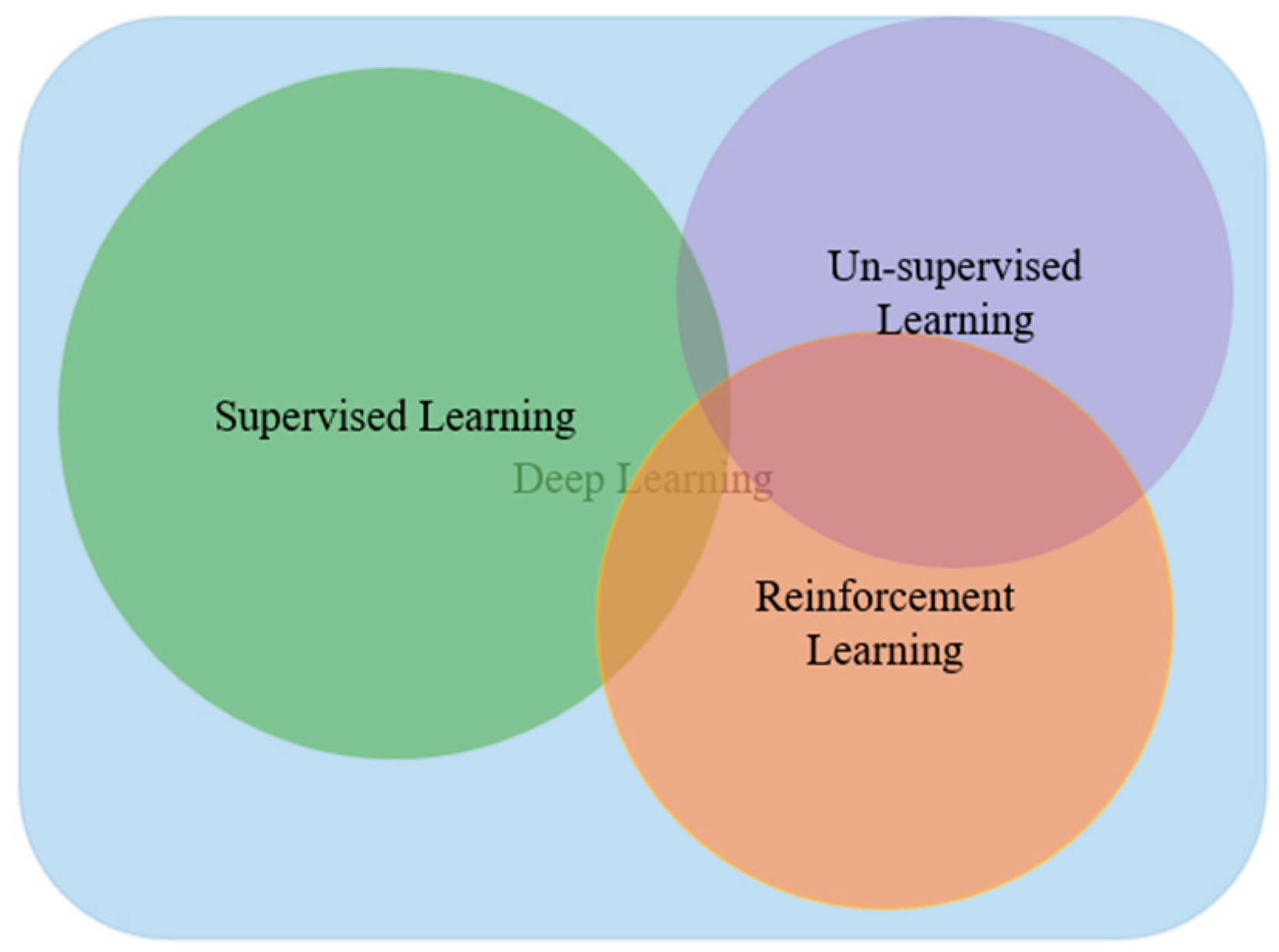
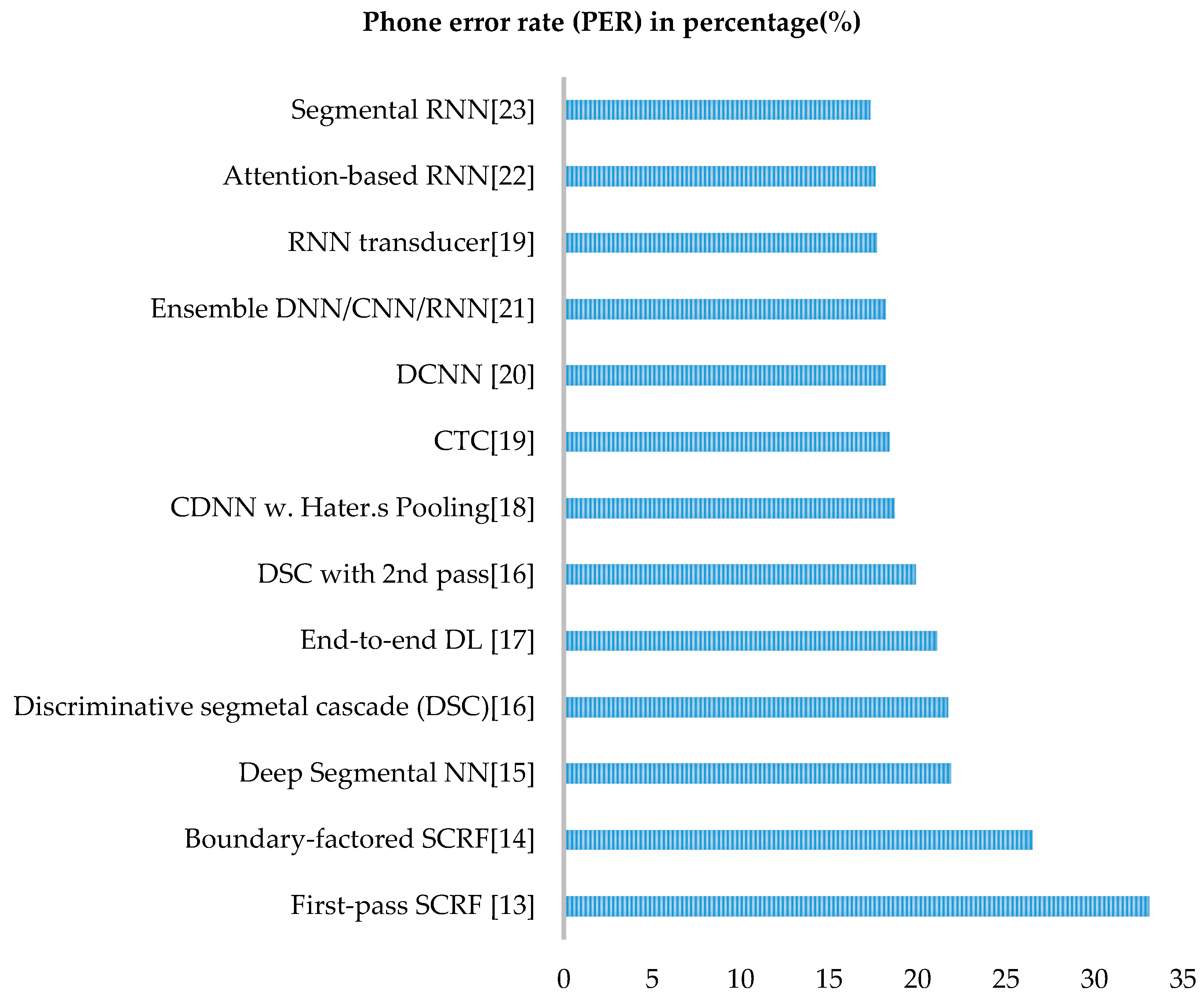
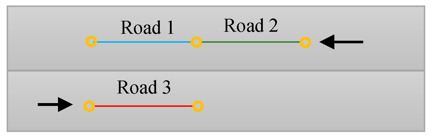
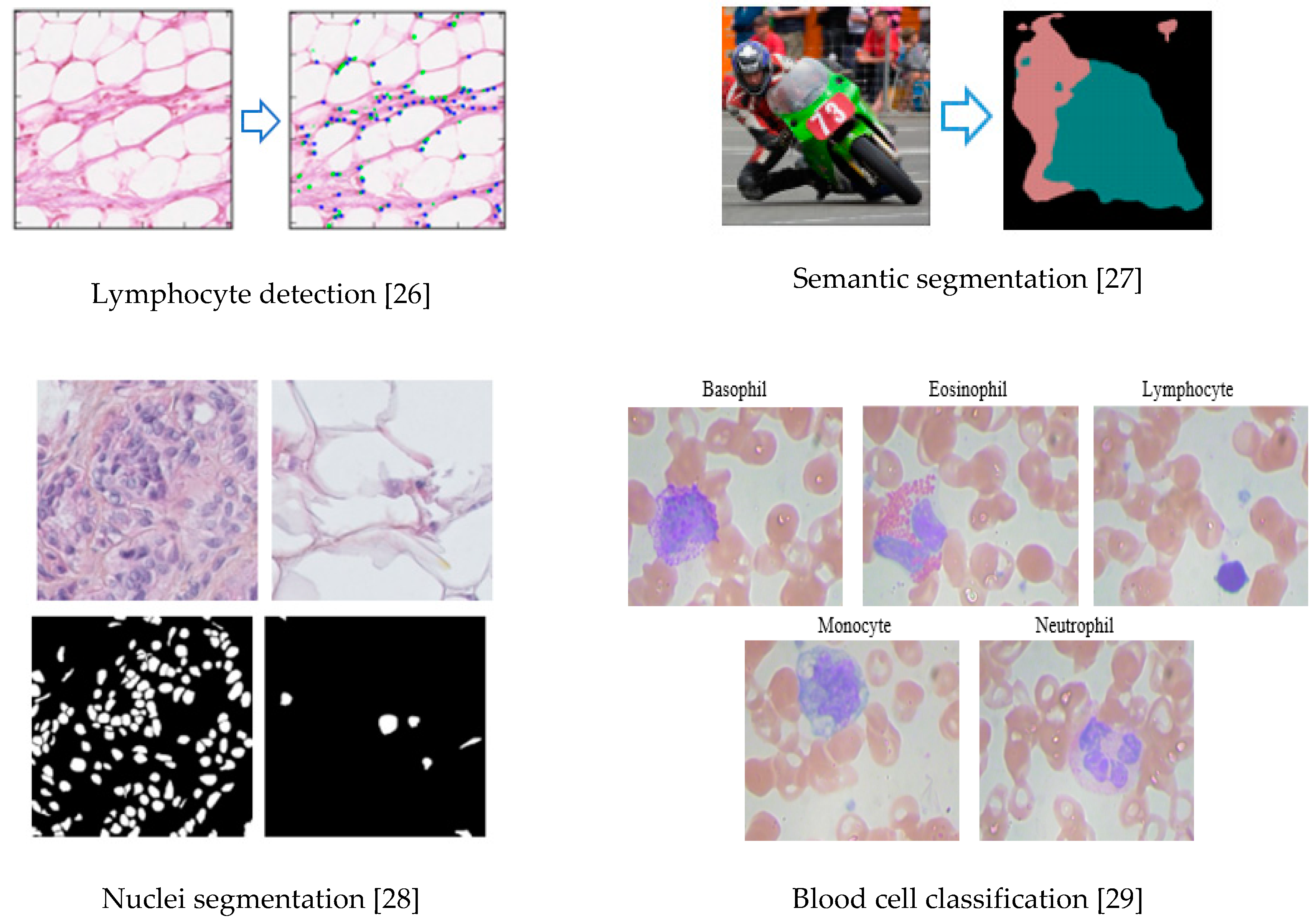
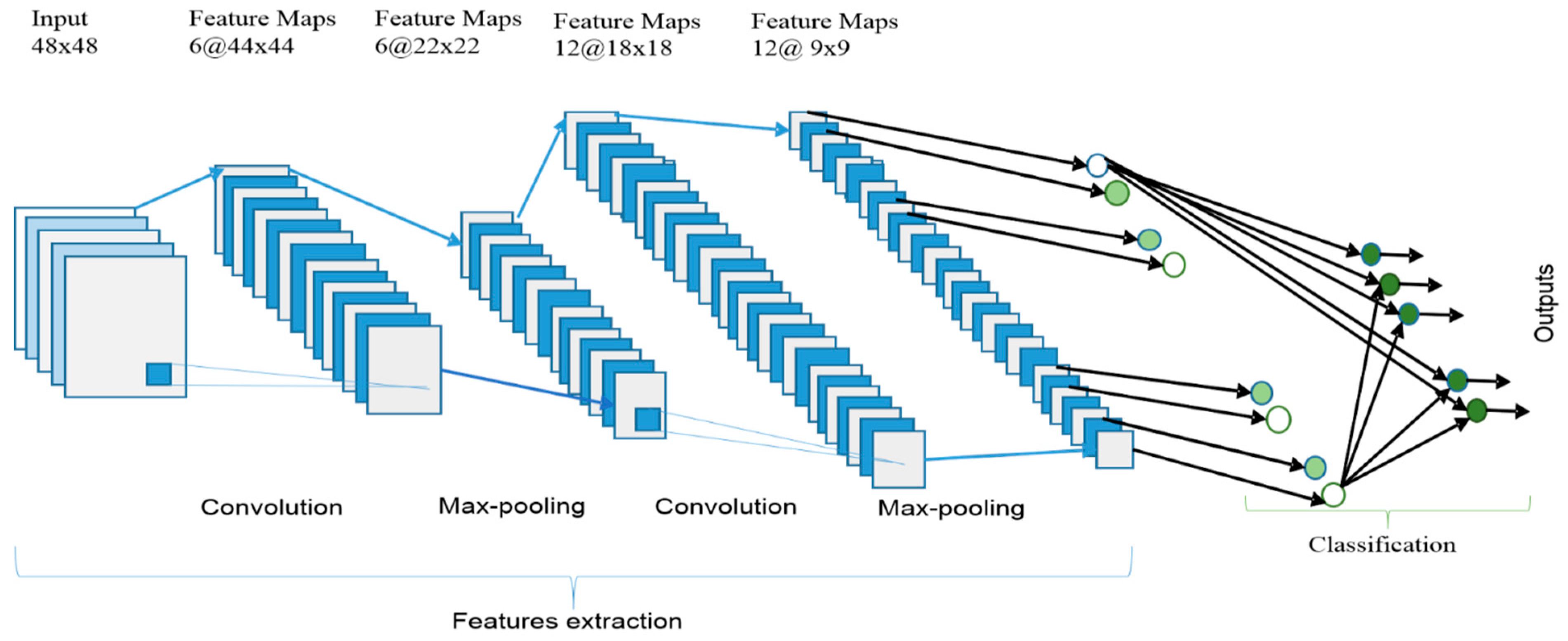
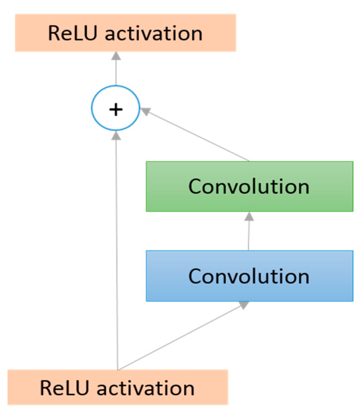
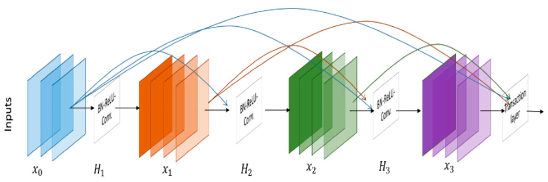
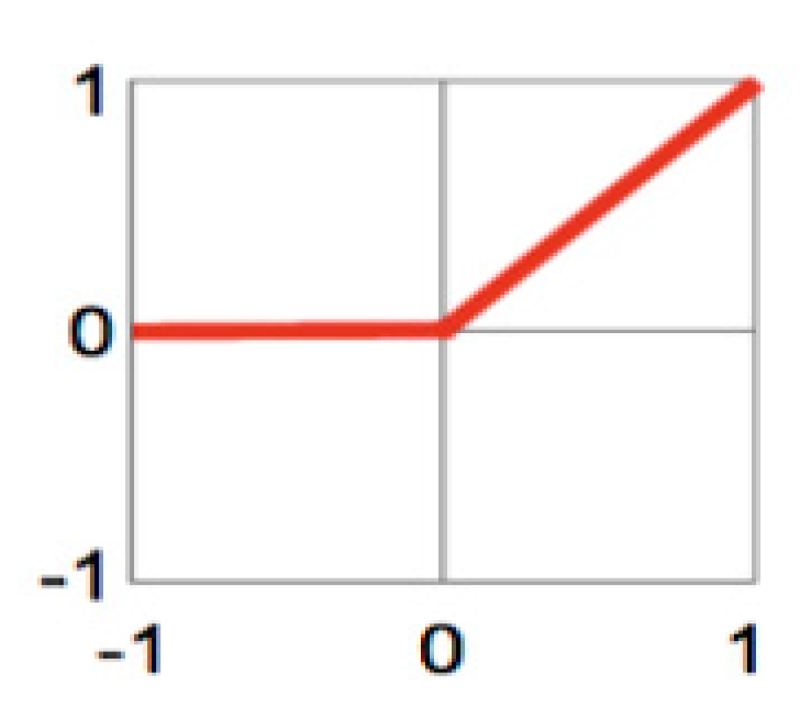
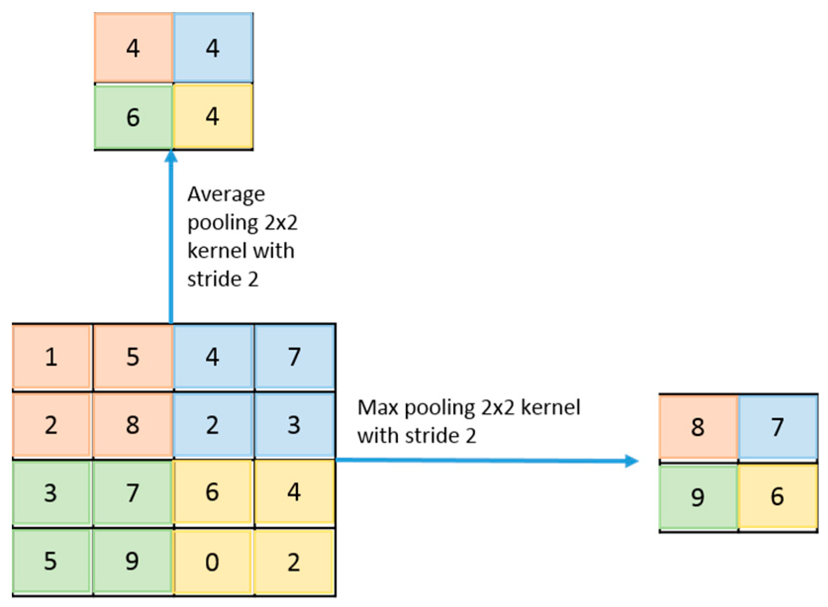
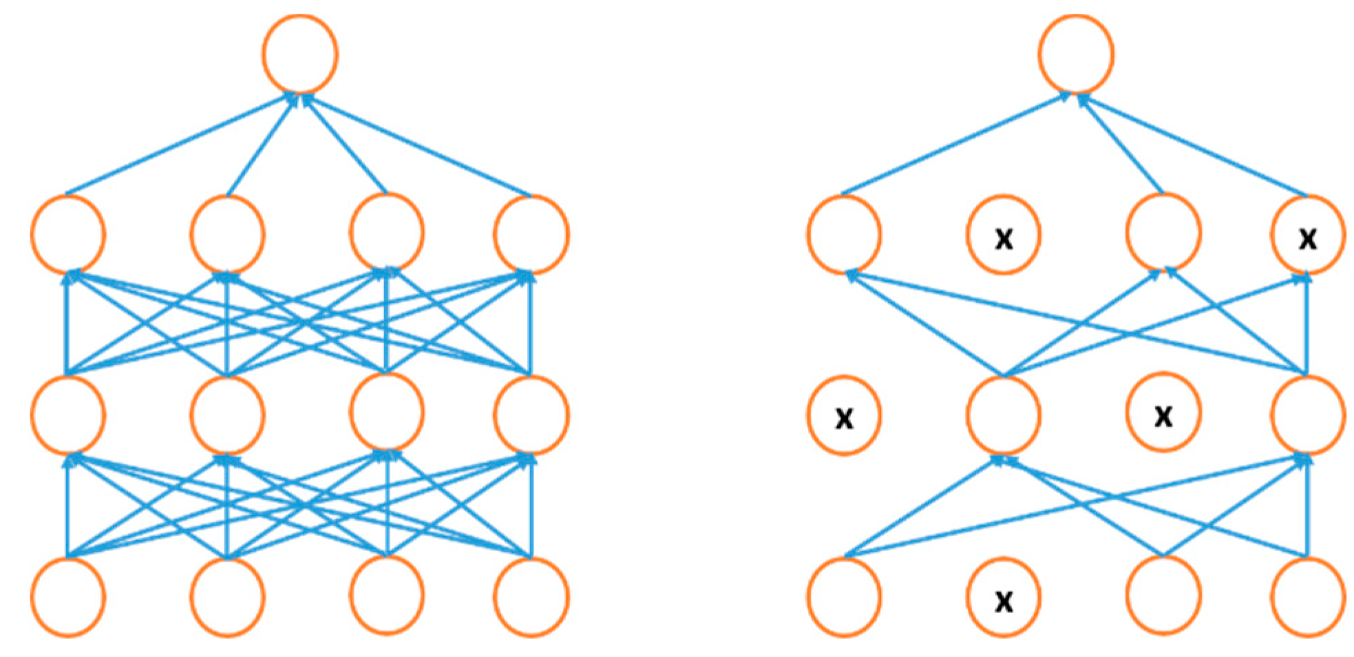
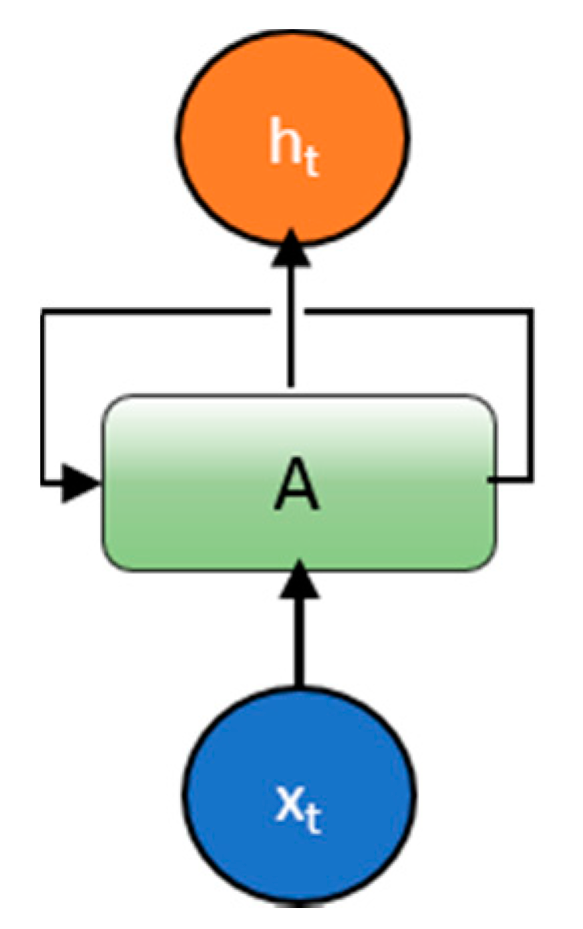
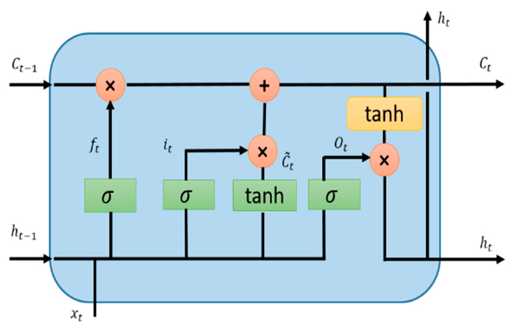
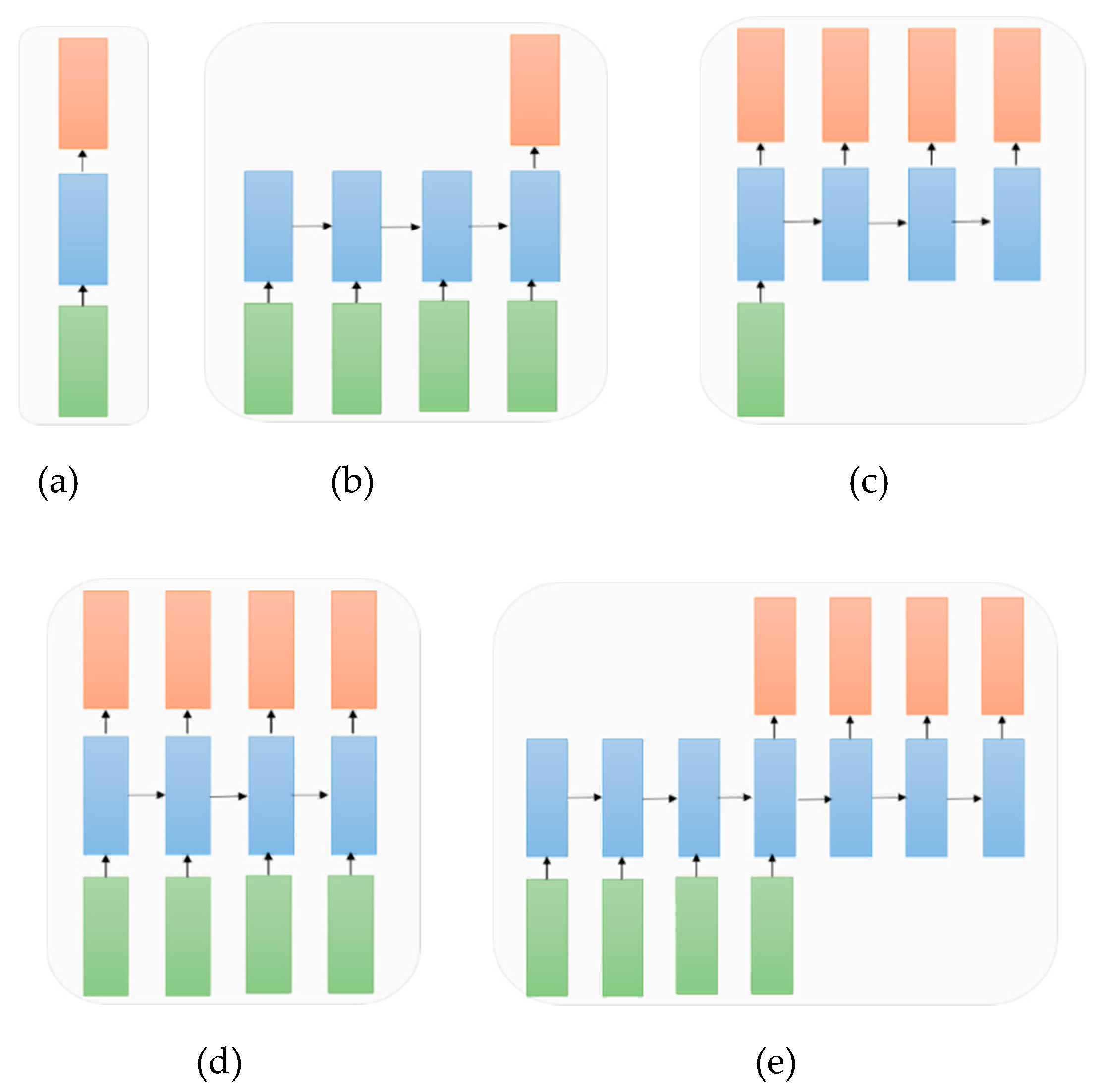
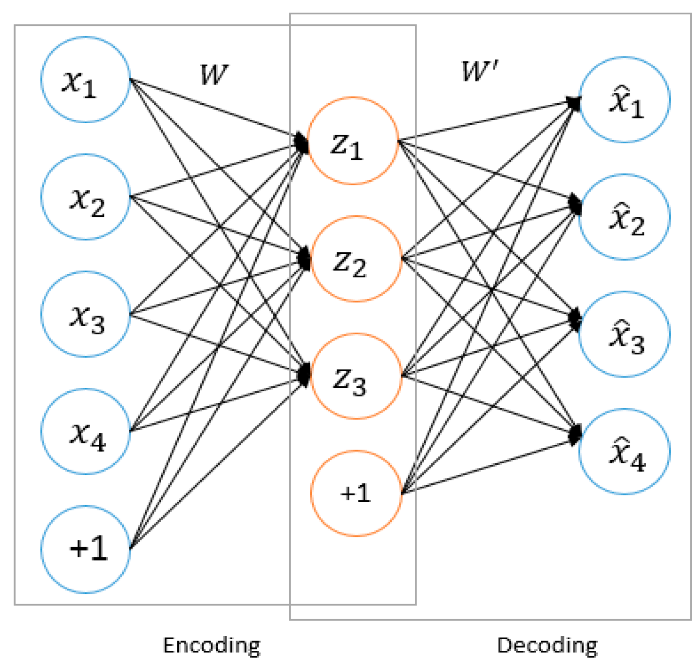
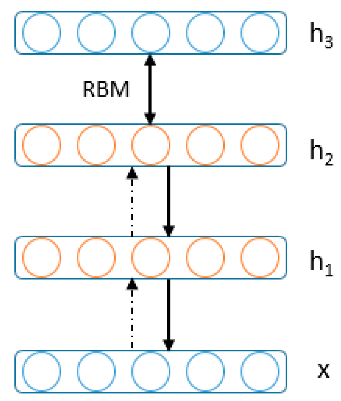
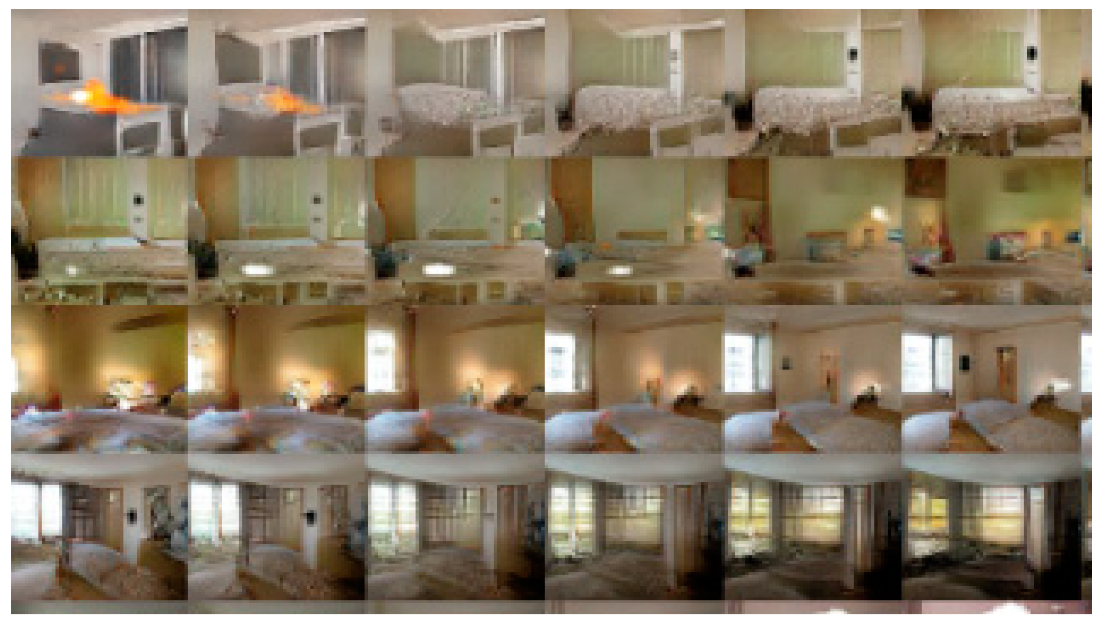
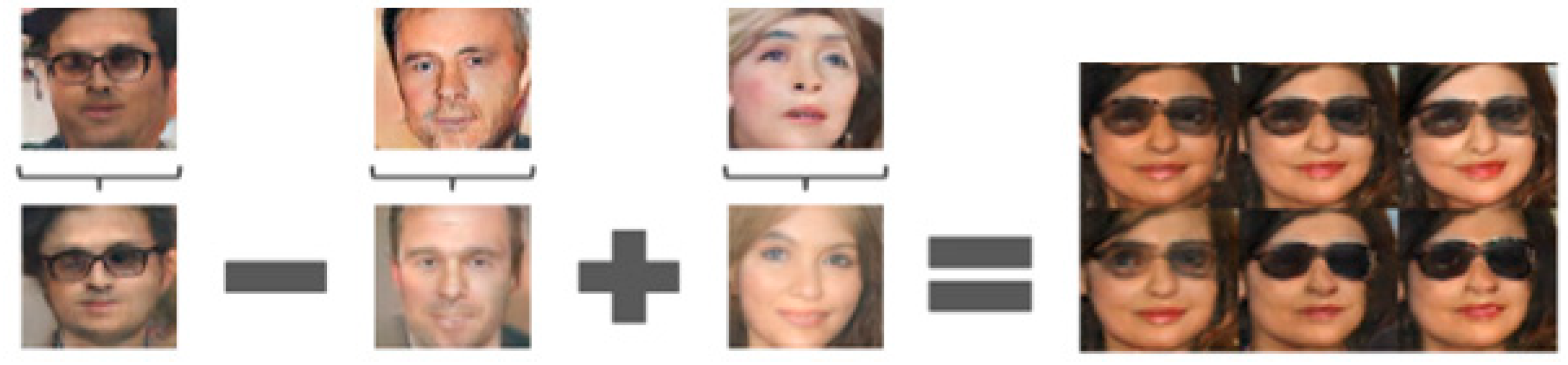
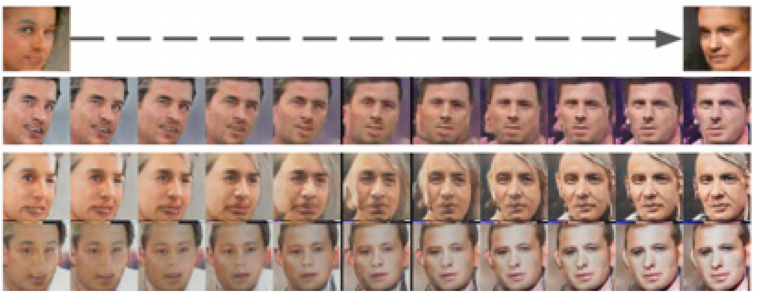
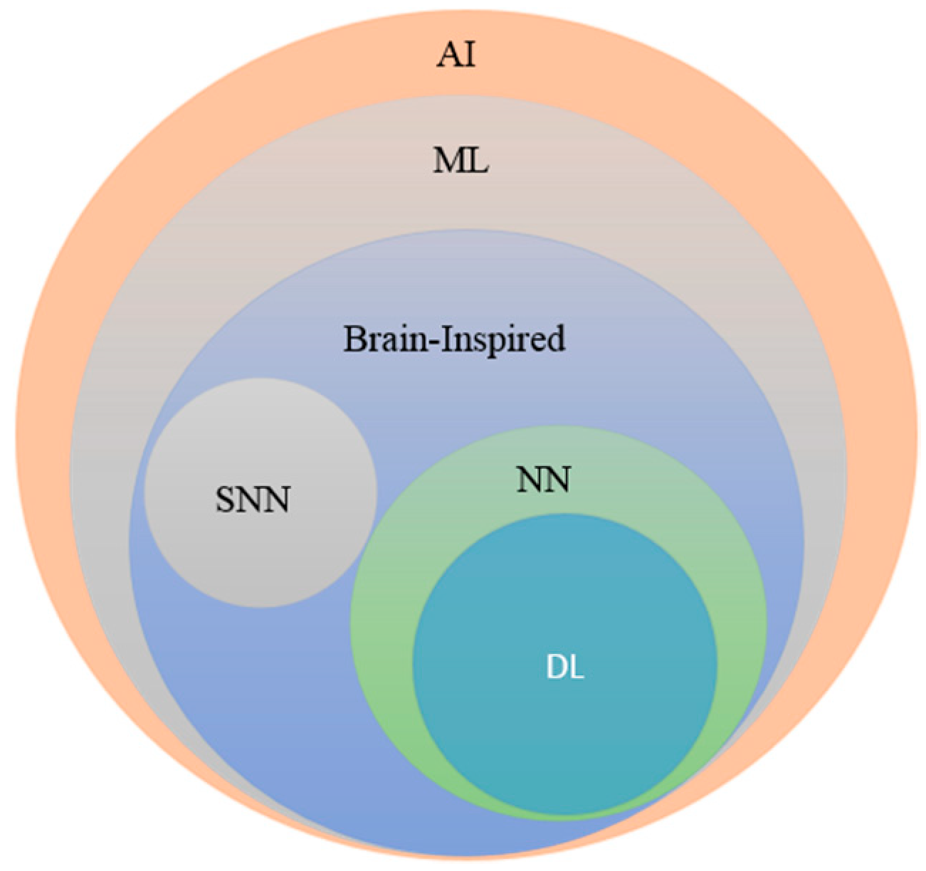
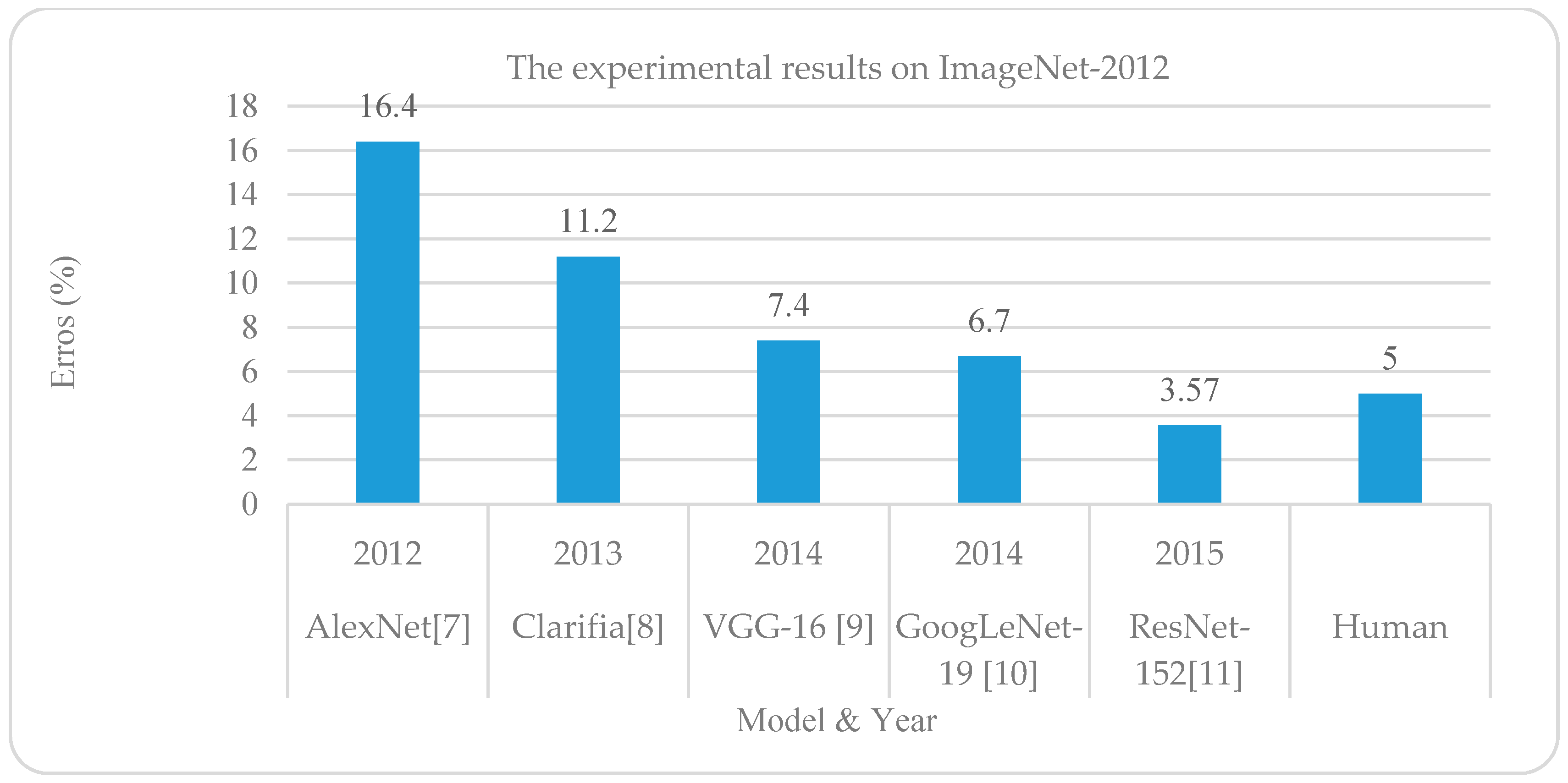
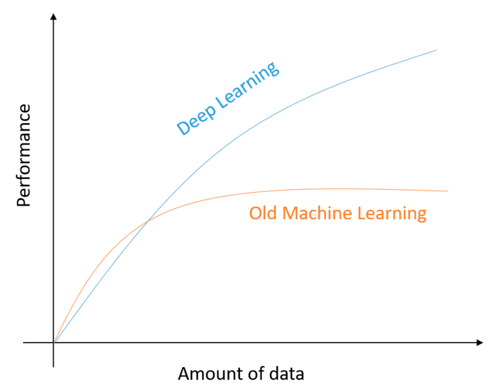
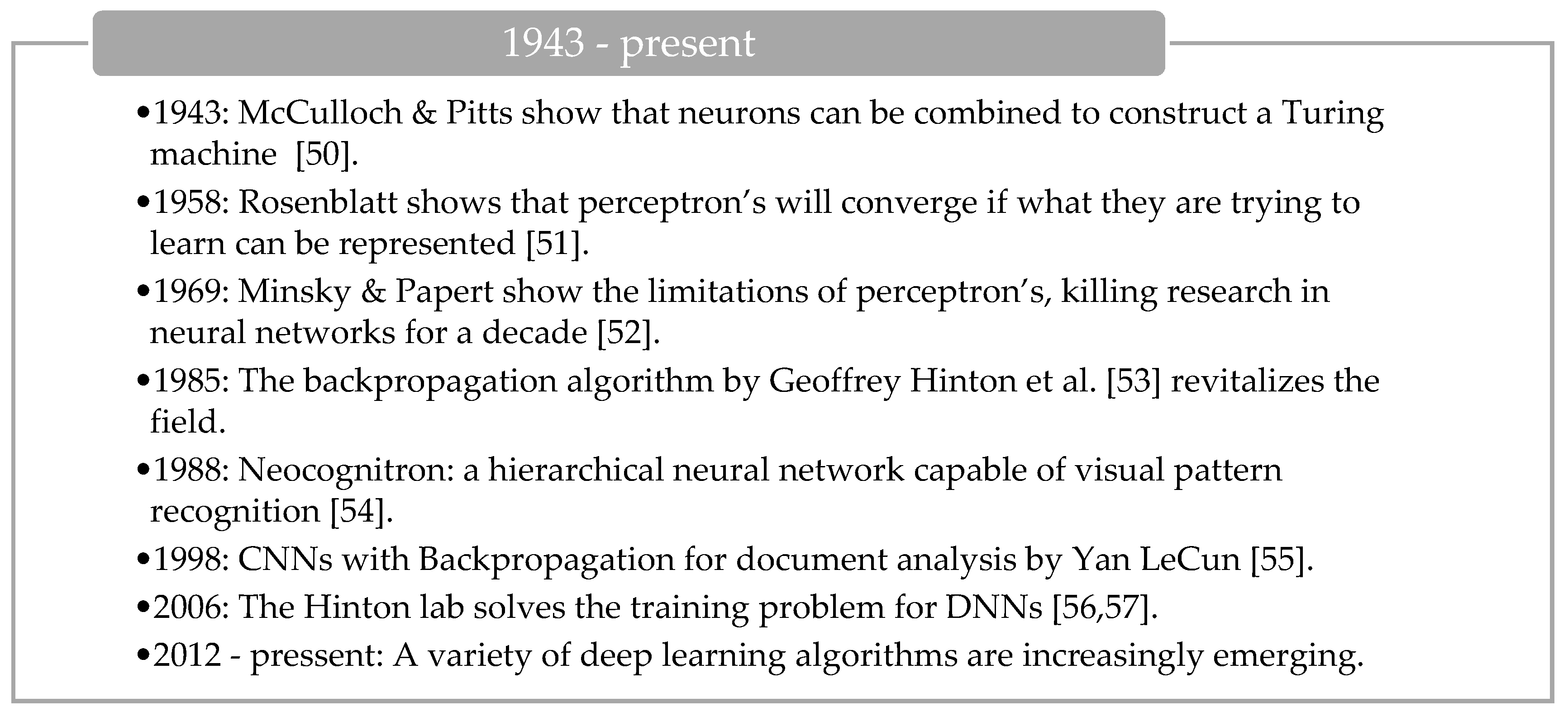
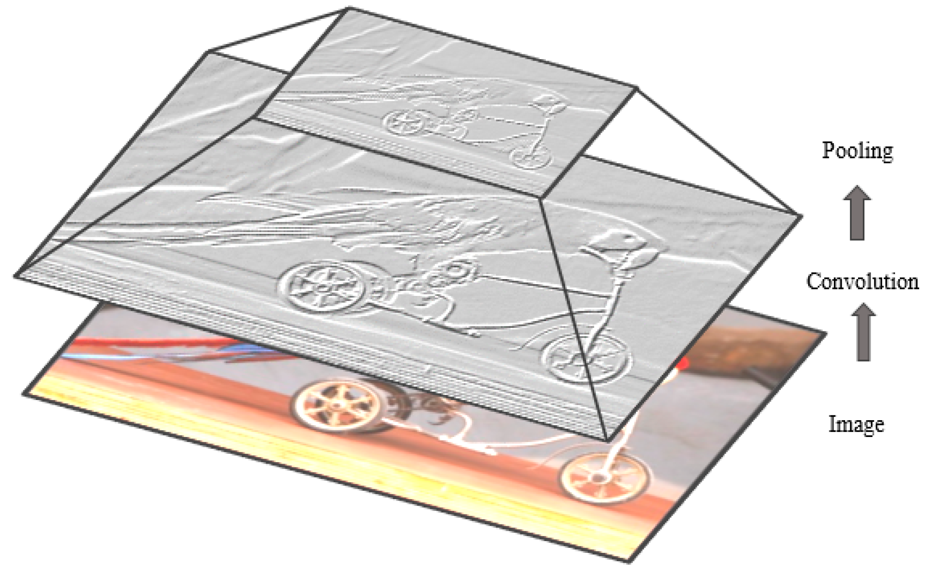
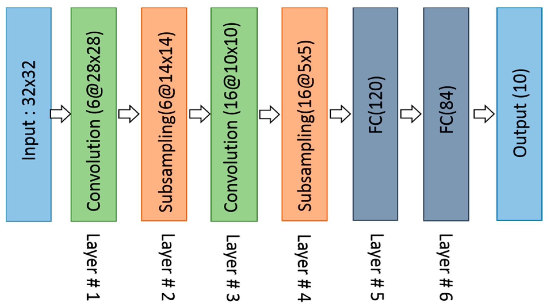
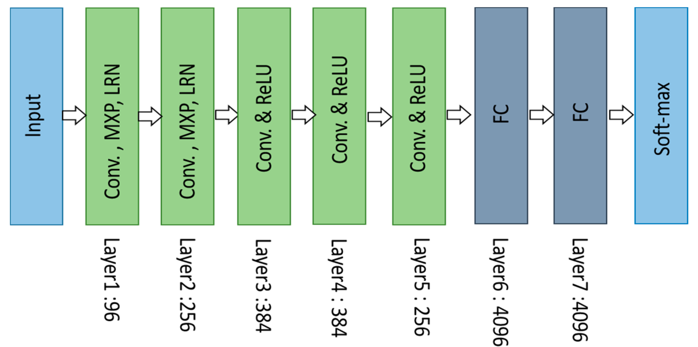
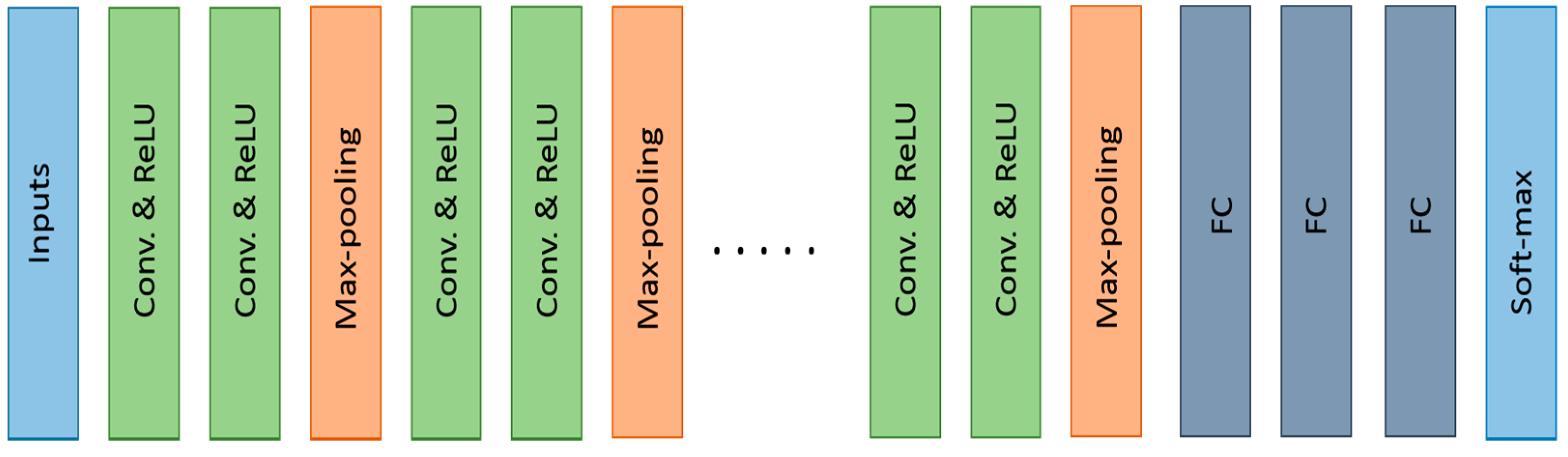
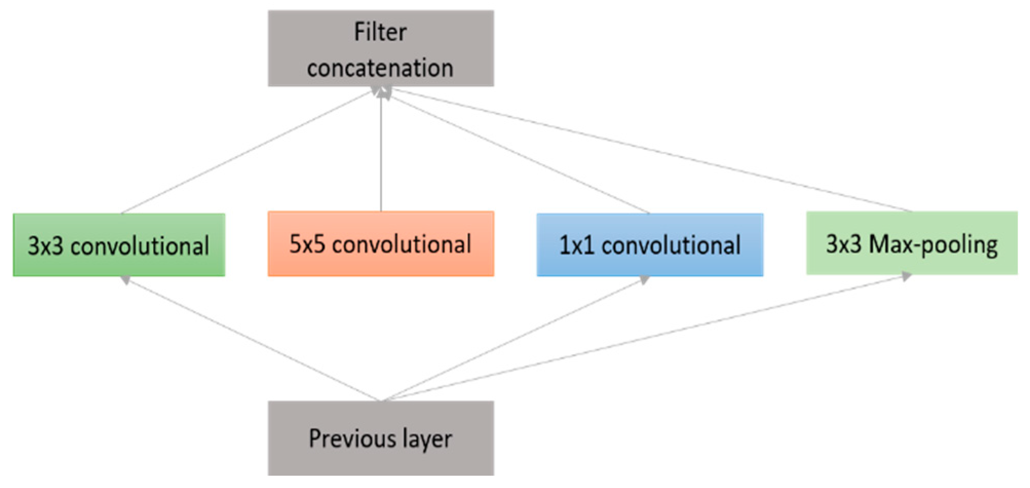
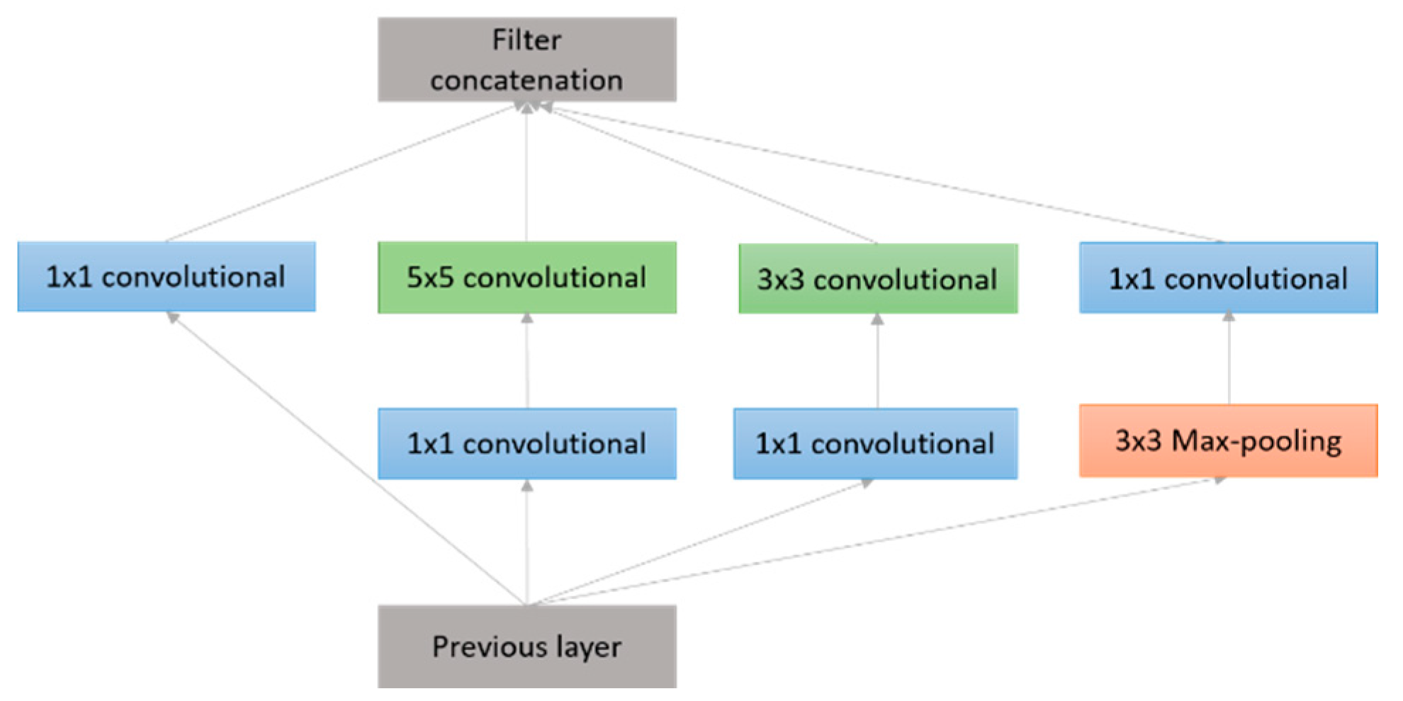
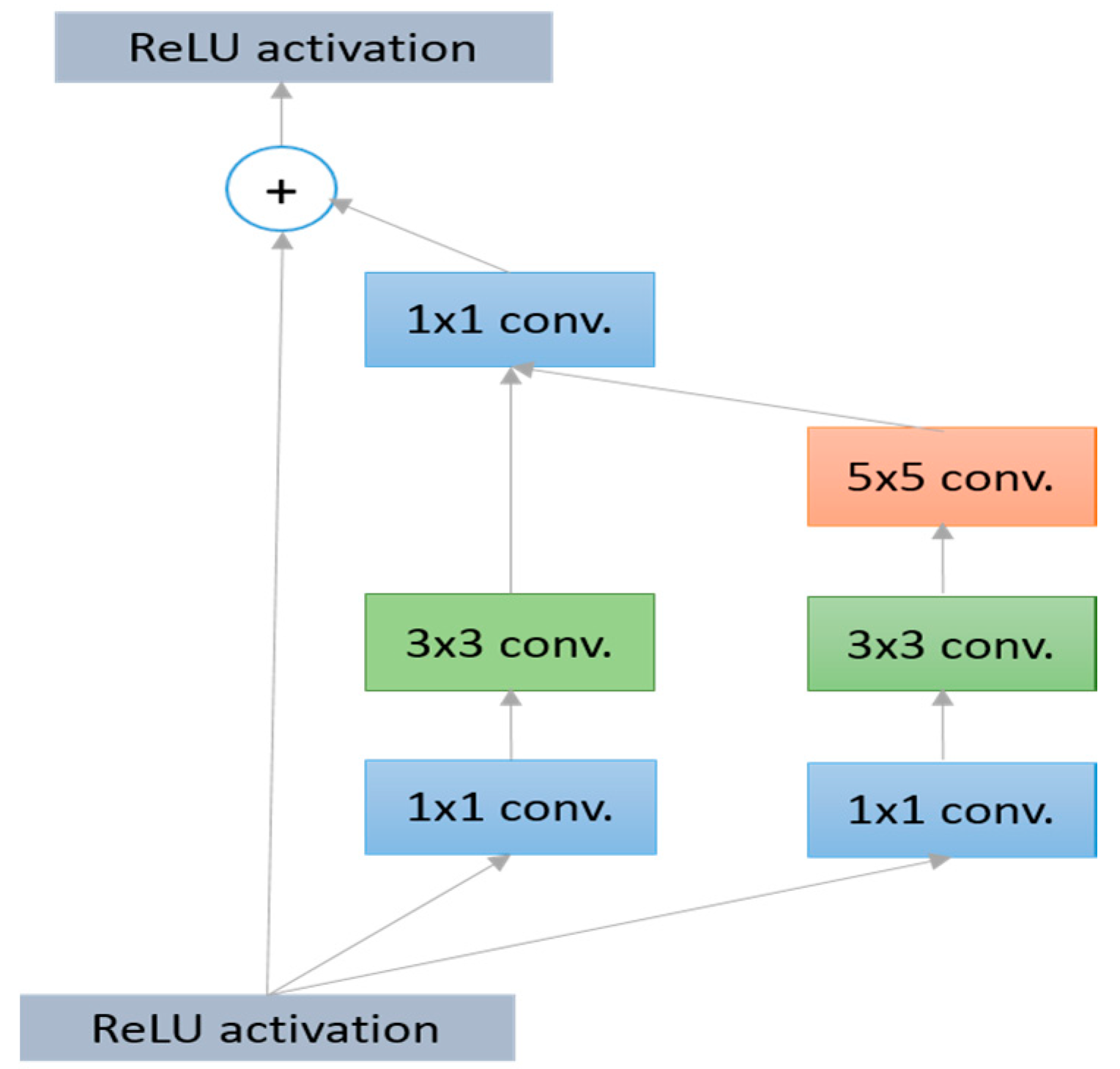
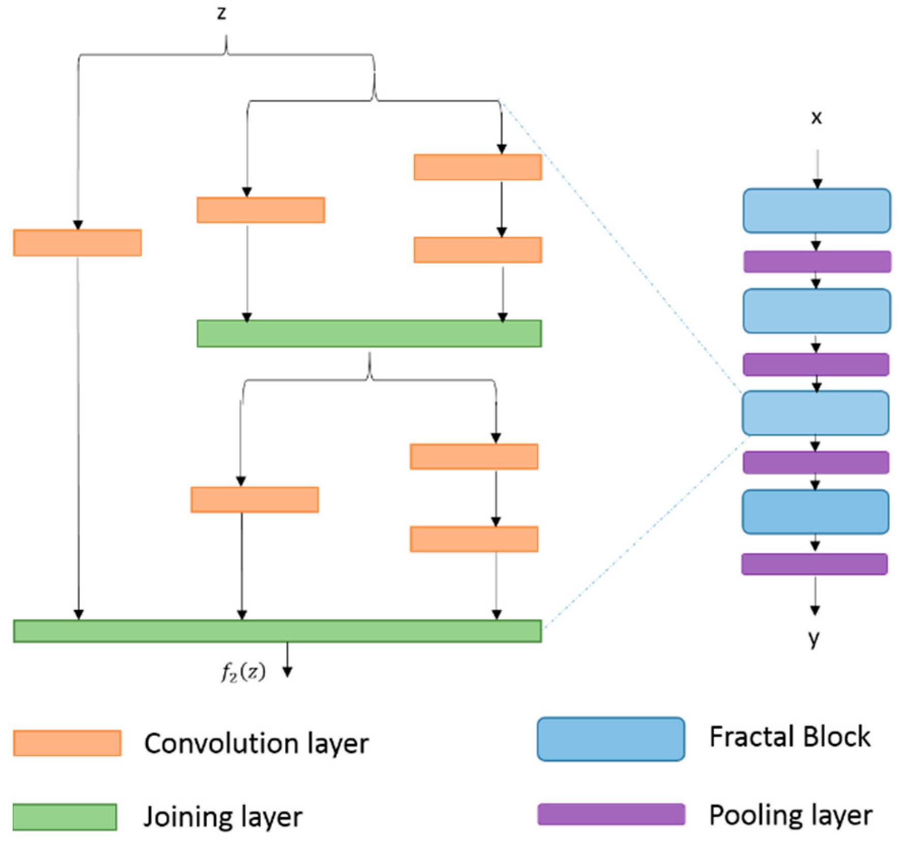
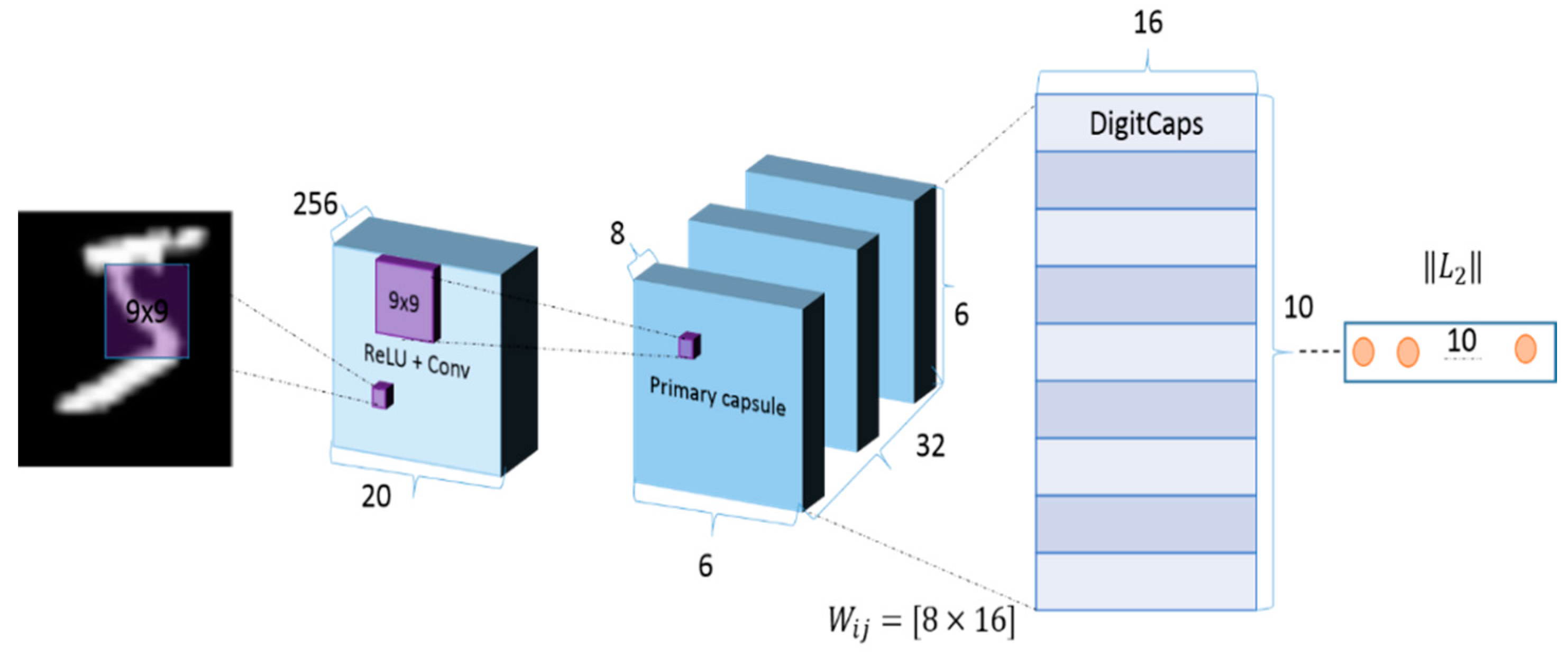
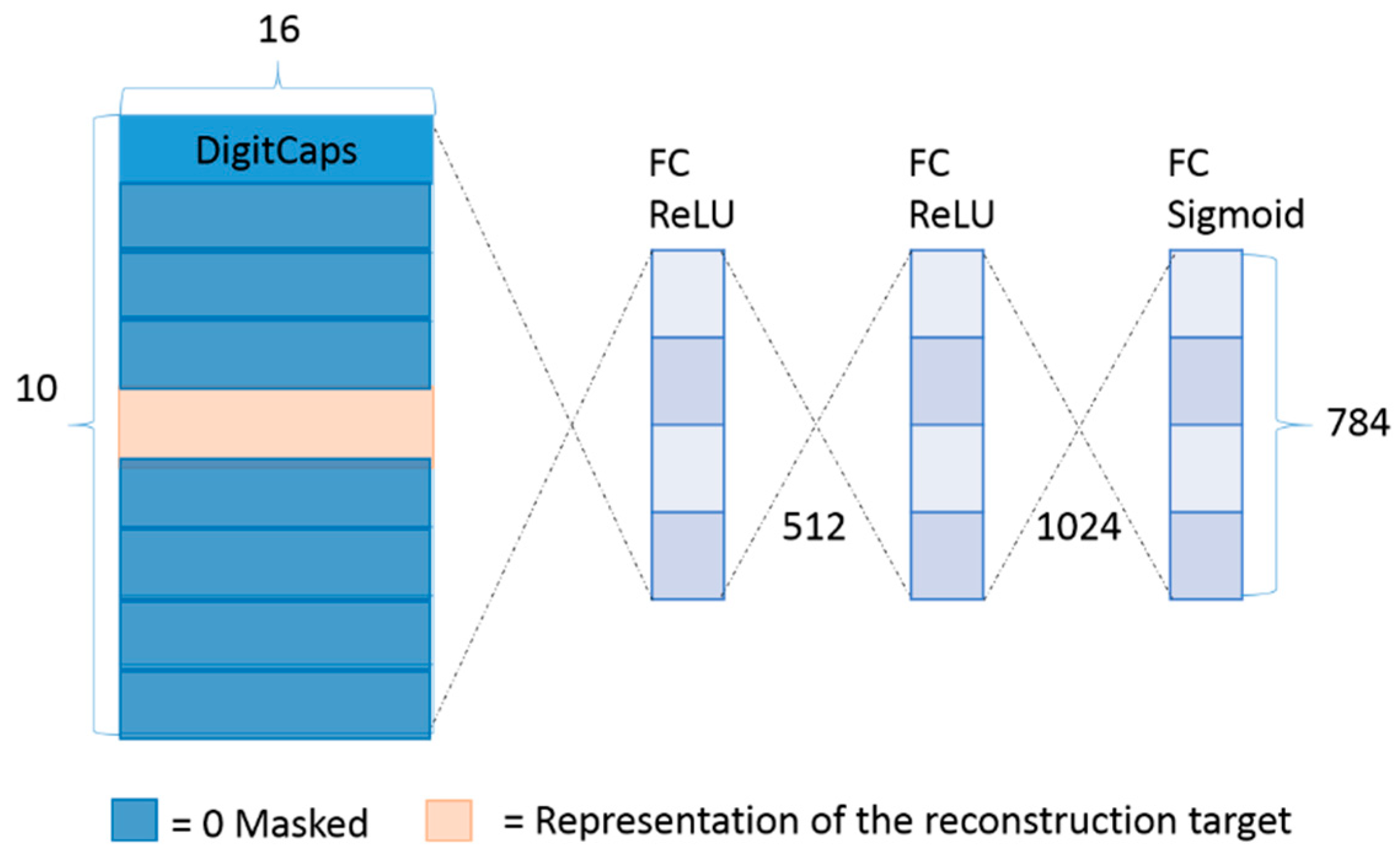
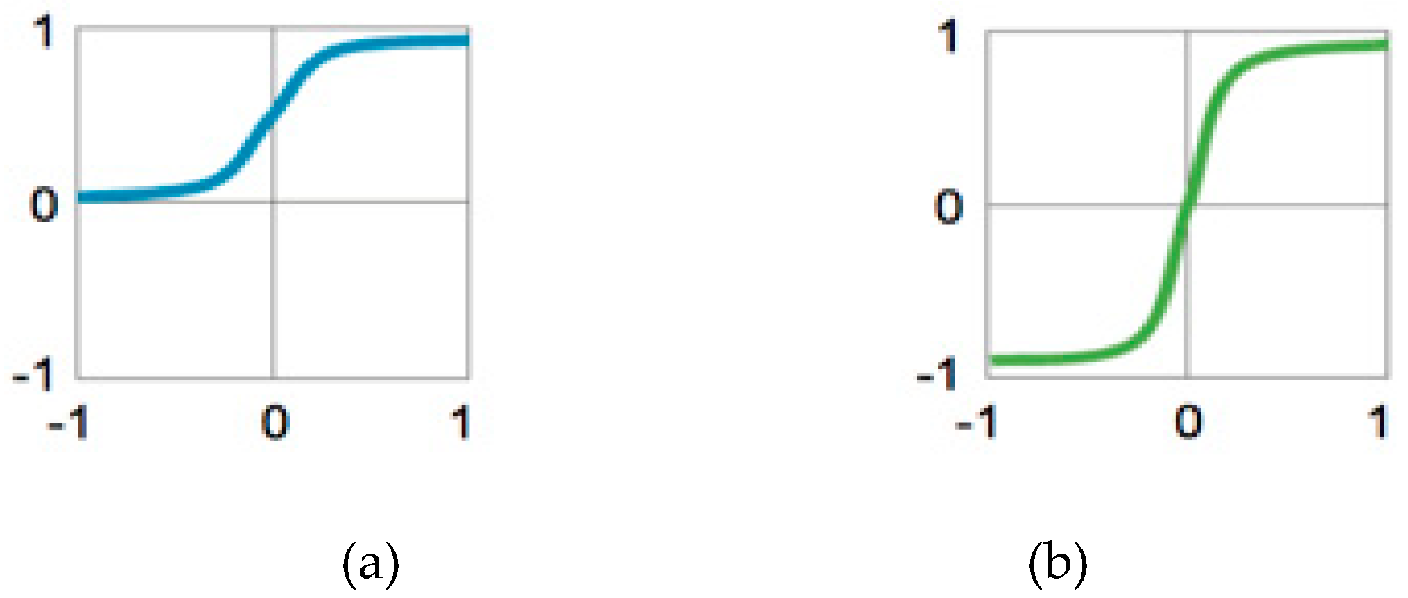
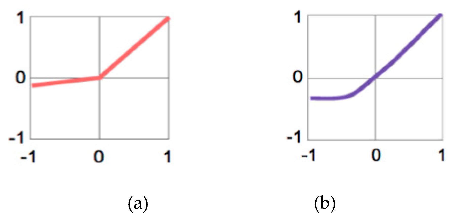
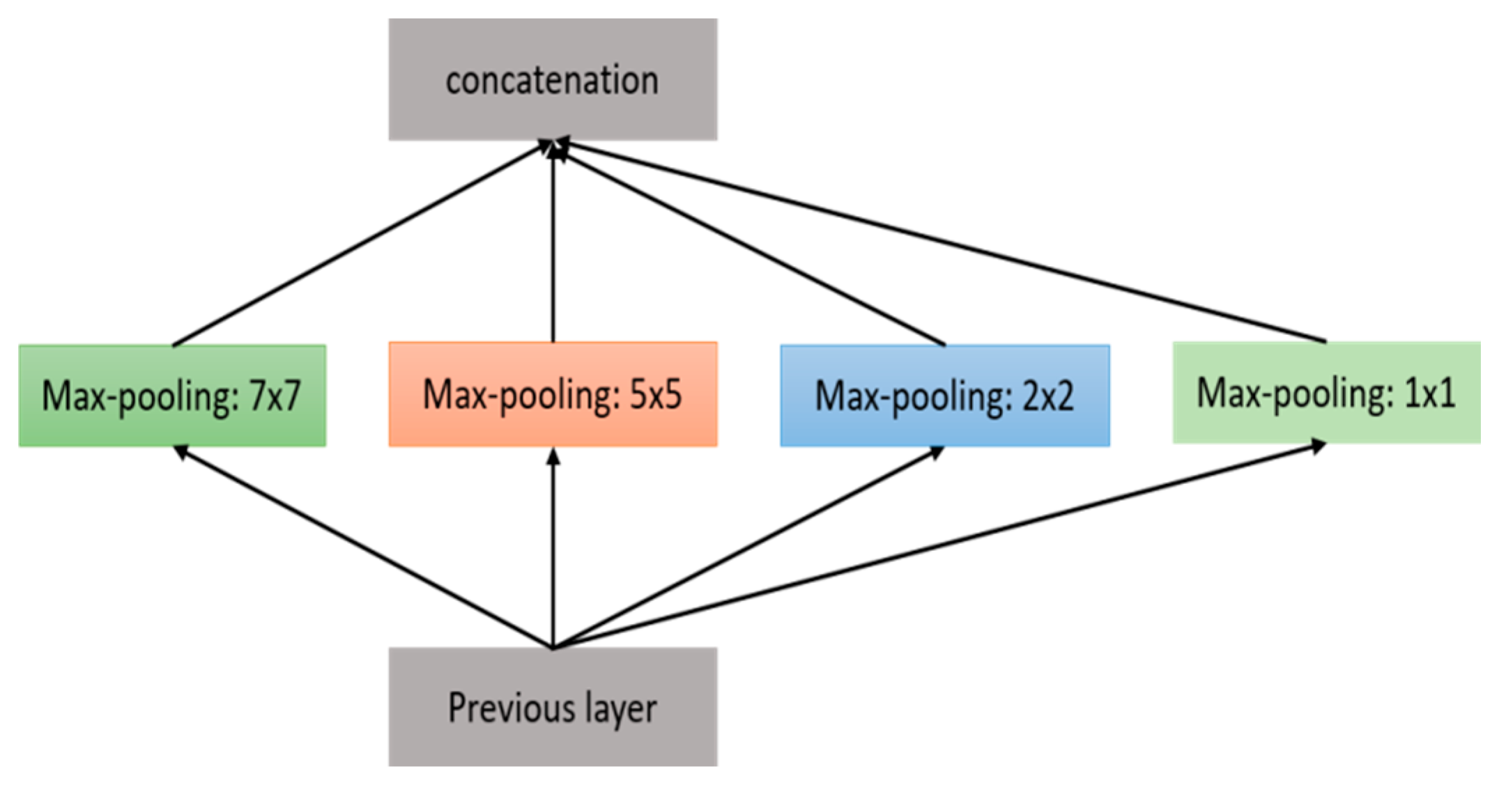
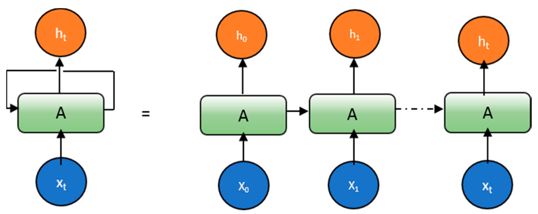
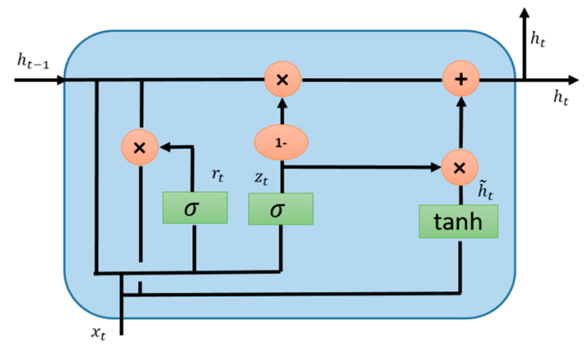
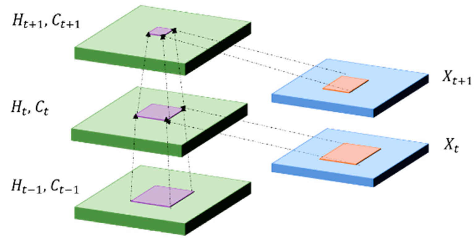
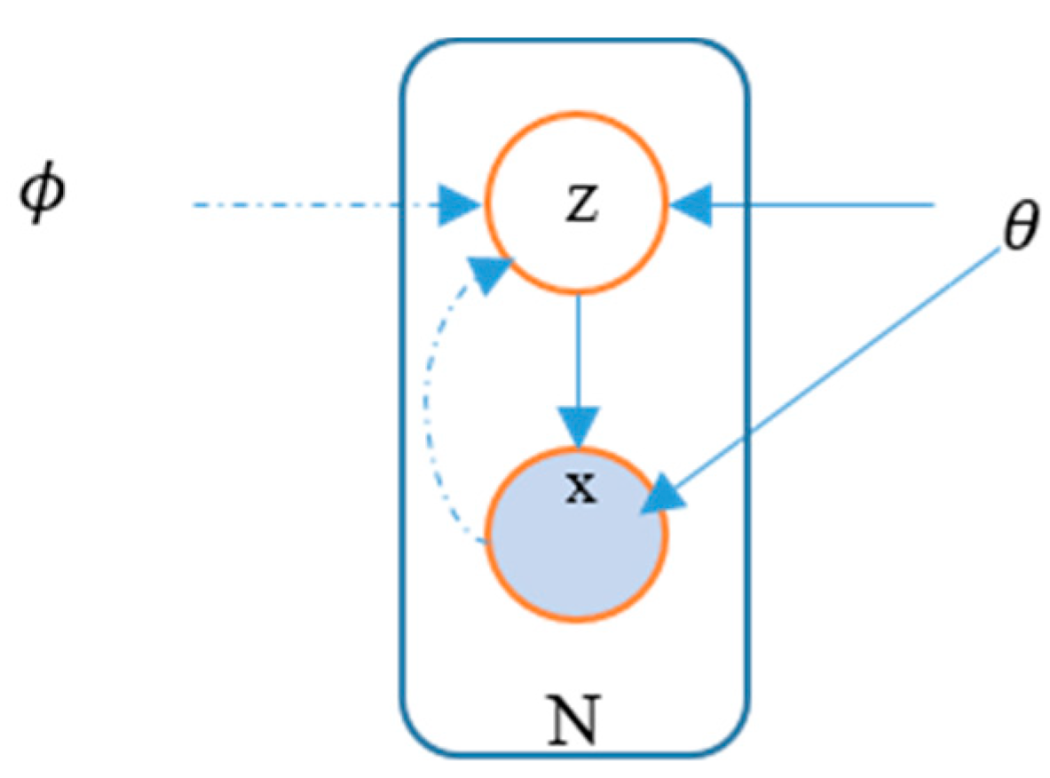
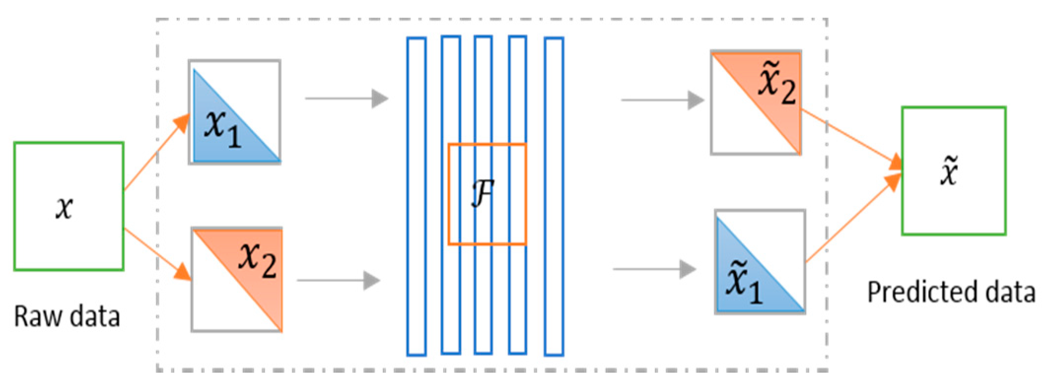
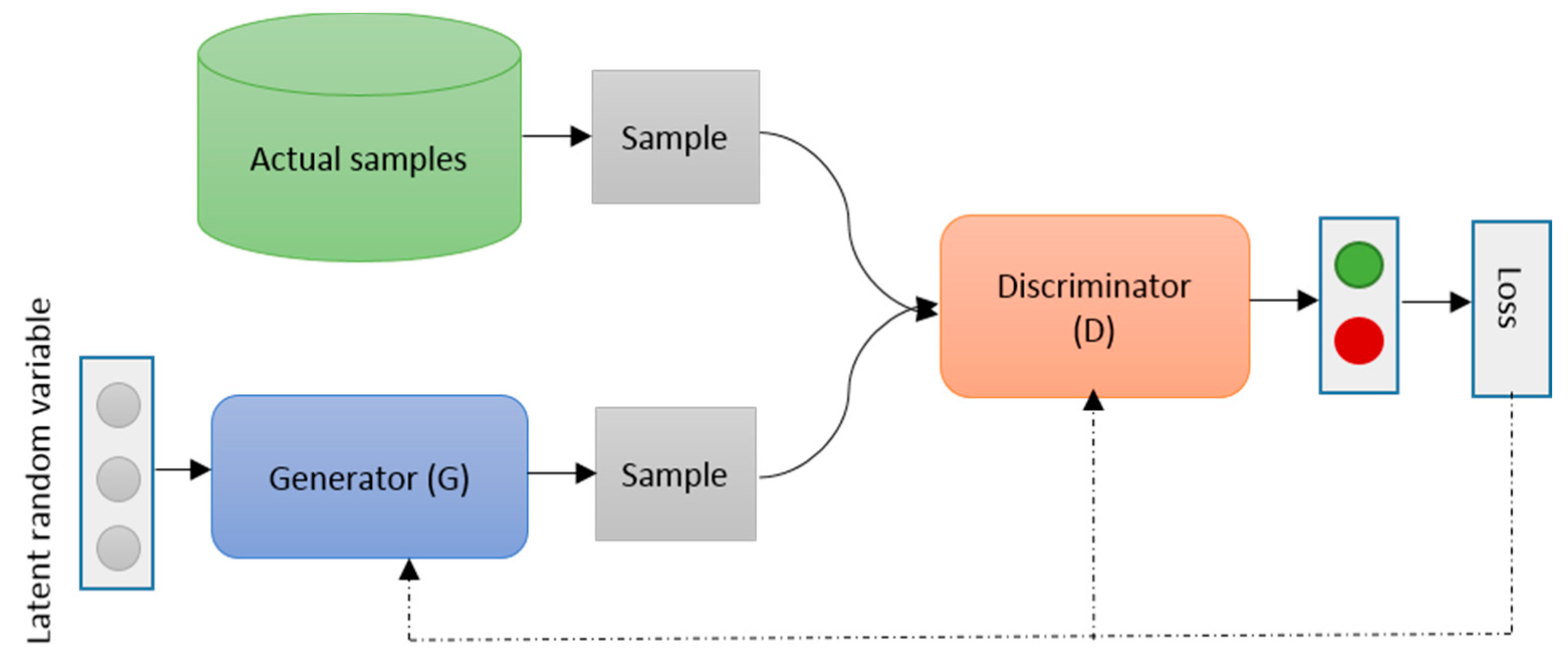
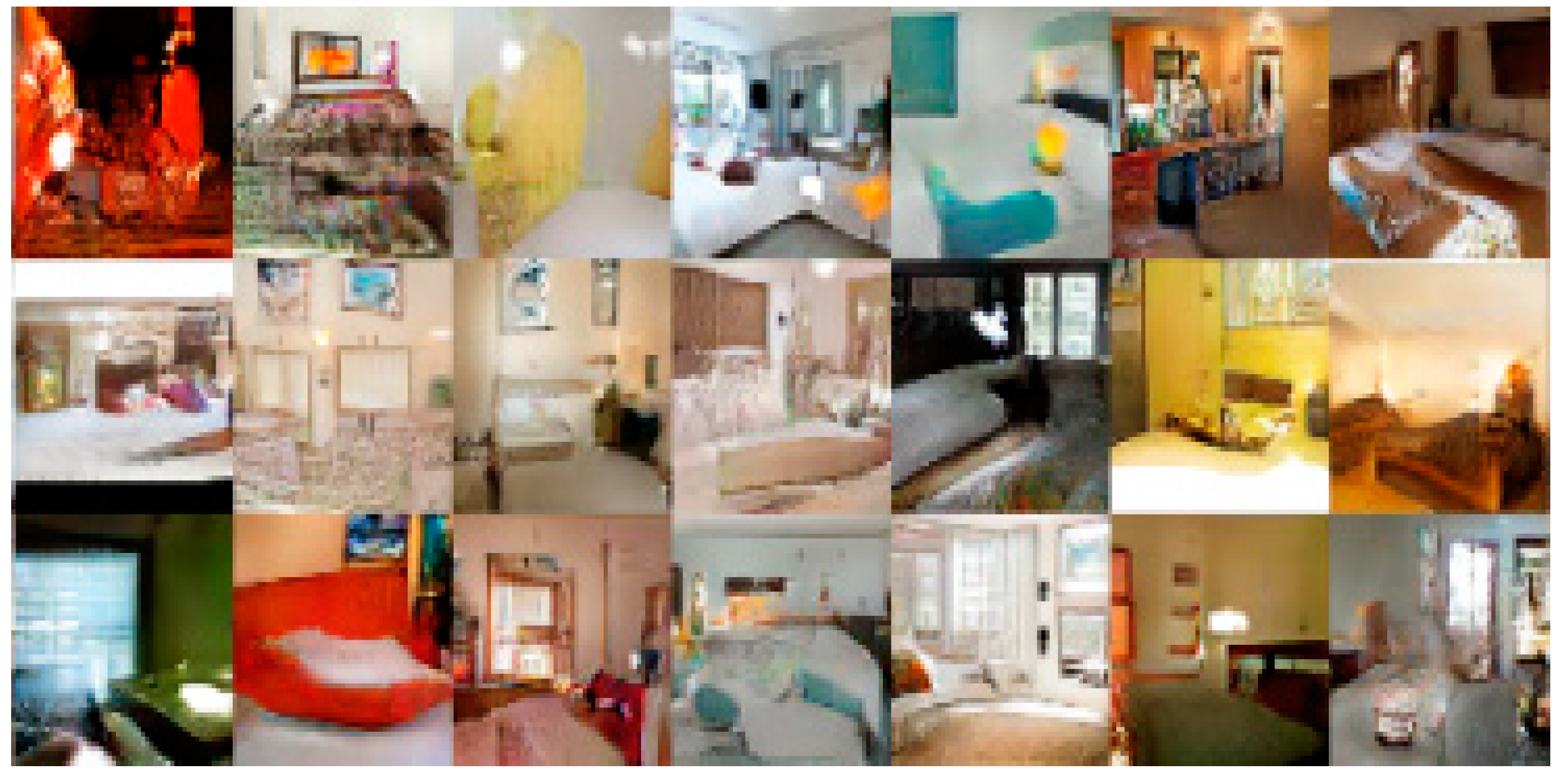
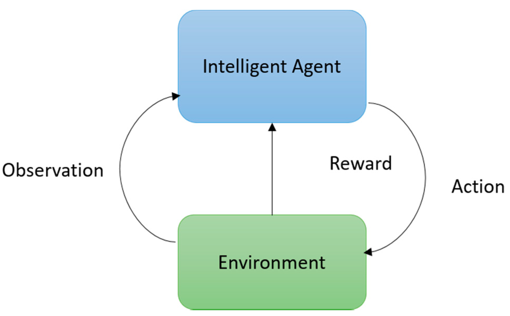
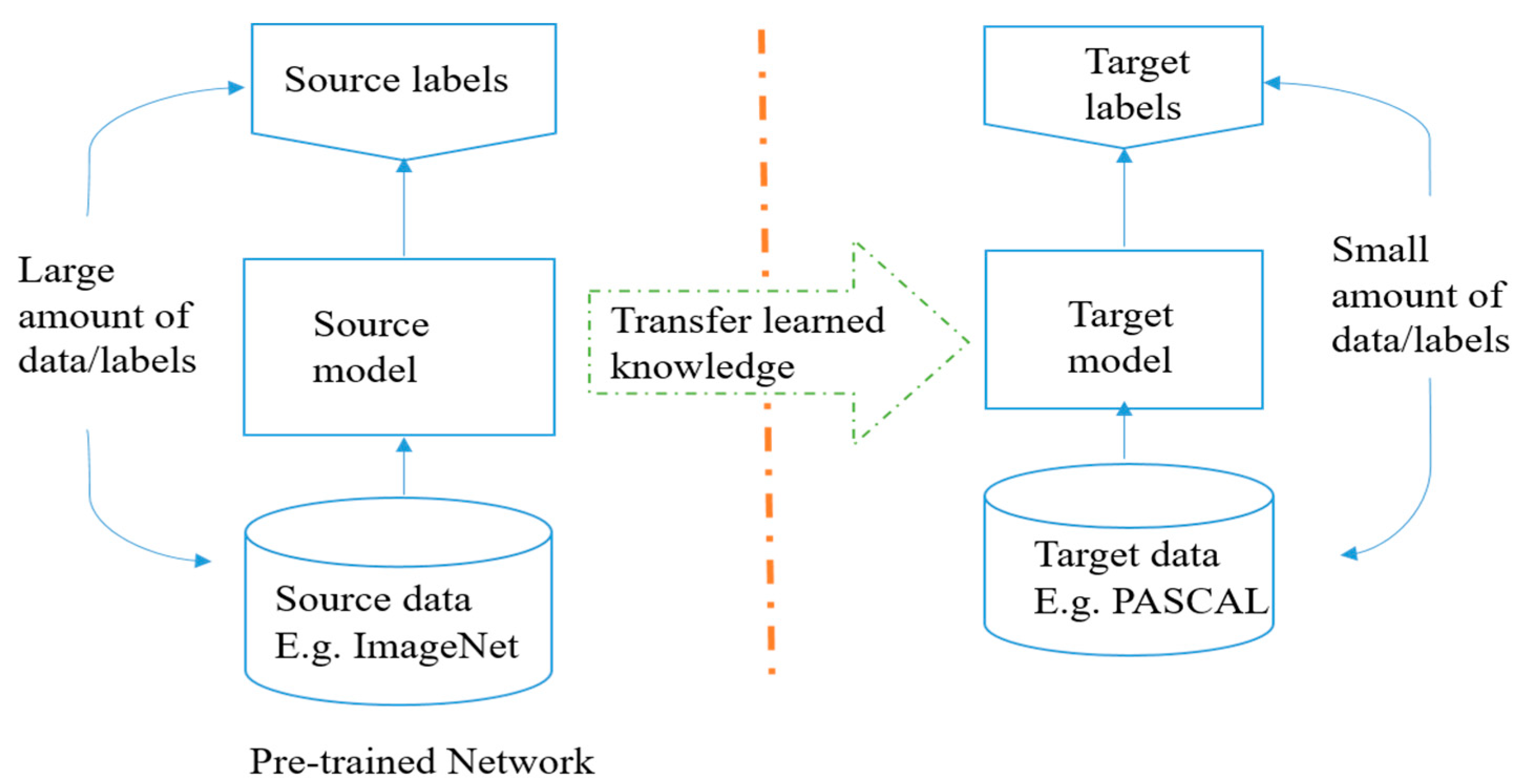
Figure 1. The taxonomy of AI. AI: Artificial Intelligence; ML: Machine Learning; NN: Neural Networks; DL: Deep Learning; SNN: Spiking Neural Networks.
Electronics 08 00292 g001
Figure 2. Category of Deep Leaning approaches.
Electronics 08 00292 g002
Figure 3. Accuracy for ImageNet classification challenge with different DL models.
Electronics 08 00292 g003
Figure 4. Phone error rate (PER) for TIMIT Acoustic-Phonetic Continuous Speech Corpus dataset [13,14,15,16,17,18,19,20,21,22,23].
Electronics 08 00292 g004
Figure 5. Data-driven traffic forecasting. Using the dynamics of the traffic flow (roads 1, 2, and 3) to capture the spatial dependency using by Diffusion Convolutional Recurrent Neural Network [25].
Electronics 08 00292 g005
Figure 6. Example images where DL is applied successfully and achieved state-of-the-art performance. The images were taken from the corresponding references [26,27,28,29].
Electronics 08 00292 g006
Figure 7. The performance of deep learning with respect to the amount of data.
Electronics 08 00292 g007
Figure 8. The history of deep learning development [50,51,52,53,54,55,56,57].
Electronics 08 00292 g008
Figure 9. The overall architecture of the Convolutional Neural Network (CNN) includes an input layer, multiple alternating convolution and max-pooling layers, one fully-connected layer and one classification layer.
Electronics 08 00292 g009
Figure 10. Feature maps after performing convolution and pooling operations.
Electronics 08 00292 g010
Figure 11. The architecture of LeNet.
Electronics 08 00292 g011
Figure 12. The architecture of AlexNet: Convolution, max-pooling, Local Response Normalization (LRN) and fully connected (FC) layer.
Electronics 08 00292 g012
Figure 13. The basic building block of VGG network: Convolution (Conv) and FC for fully connected layers.
Electronics 08 00292 g013
Figure 14. Inception layer: Naive version.
Electronics 08 00292 g014
Figure 15. Inception layer with dimension reduction.
Electronics 08 00292 g015
Figure 16. Basic diagram of the Residual block.
Electronics 08 00292 g016
Figure 17. The basic block diagram for Inception Residual unit.
Electronics 08 00292 g017
Figure 18. A 4-layer Dense block with a growth rate of k = 3 .
Electronics 08 00292 g018
Figure 19. The detailed FractalNet module on the left and FractalNet on the right.
Electronics 08 00292 g019
Figure 20. A CapsNet encoding unit with 3 layers. The instance of each class is represented with a vector of a capsule in DigitCaps layer that is used for calculating classification loss. The weights between the primary capsule layer and DigitCaps layer are represented with W i j .
Electronics 08 00292 g020
Figure 21. The decoding unit where a digit is reconstructed from DigitCaps layer representation. The Euclidean distance is used minimizing the error between the input sample and the reconstructed sample from the sigmoid layer. True labels are used for reconstruction target during training.
Electronics 08 00292 g021
Figure 22. Activation function: (a) Sigmoid function, and (b) hyperbolic transient.
Electronics 08 00292 g022
Figure 23. Pictorial representation of Rectified Linear Unit (ReLU).
Electronics 08 00292 g023
Figure 24. Diagram for (a) Leaky ReLU (Rectified Linear Unit), and (b) Exponential Linear Unit (ELU).
Electronics 08 00292 g024
Figure 25. Average and max-pooling operations.
Electronics 08 00292 g025
Figure 26. Spatial pyramid pooling.
Electronics 08 00292 g026
Figure 27. Pictorial representation of the concept Dropout.
Electronics 08 00292 g027
Figure 28. The structure of basic Recurrent Neural Network (RNN) with a loop.
Electronics 08 00292 g028
Figure 29. An unrolled RNNs.
Electronics 08 00292 g029
Figure 30. Diagram for Long Short-Term Memory (LSTM).
Electronics 08 00292 g030
Figure 31. Diagram for Gated Recurrent Unit (GRU).
Electronics 08 00292 g031
Figure 32. Pictorial diagram for ConvLSTM.
Electronics 08 00292 g032
Figure 33. The different structure of RNN with respect to the applications: (a) One to one; (b) many to one; (c) one to many; (d) many to many; and (e) many to many.
Electronics 08 00292 g033
Figure 34. Diagram for Auto encoder.
Electronics 08 00292 g034
Figure 35. Variational Auto-Encoder.
Electronics 08 00292 g035
Figure 36. Split-Brain Autoencoder.
Electronics 08 00292 g036
Figure 37. Block diagram for Restricted Boltzmann Machine (RBM).
Electronics 08 00292 g037
Figure 38. Conceptual diagram for Generative Adversarial Networks (GAN).
Electronics 08 00292 g038
Figure 39. Experimental outputs of bedroom images.
Electronics 08 00292 g039
Figure 40. Reconstructed bedroom images using deep convolution GAN (DCGAN).
Electronics 08 00292 g040
Figure 41. Example of smile arithmetic and arithmetic for wearing glass using GAN: a man with glasses minus man without glasses plus woman without glasses equal to woman with glasses.
Electronics 08 00292 g041
Figure 42. Face generation in different angle using GAN.
Electronics 08 00292 g042
Figure 43. Conceptual diagram for Reinforcement Learning (RL) system.
Electronics 08 00292 g043
Figure 44. Conceptual diagram for transfer learning: Pretrained on ImageNet and transfer learning is used for retraining on PASCAL dataset.
Electronics 08 00292 g044
Table 1. Different feature learning approaches.
ApproachesLearning Steps
Rule-based InputHand-design featuresOutput
Traditional Machine LearningInputHand-design features Mapping from featuresOutput
Representation LearningInputFeaturesMapping from featuresOutput
Deep LearningInputSimple featuresComplex featuresMapping from featuresOutput
Table 2. The top-5% errors with computational parameters and macs for different deep CNN models.
MethodsLeNet-5 [54]AlexNet [7]OverFeat (fast) [8]VGG-16 [9]GoogLeNet [10]ResNet-50(v1) [11]
Top-5 errorsn/a16.414.27.46.75.3
Input size28 × 28227 × 227231 × 231224 × 224224 × 224224 × 224
Number of Conv Layers255162150
Filter Size53,5,113,731,3,5,71,3,7
Number of Feature Maps1,63–2563–10243–5123–10243–1024
Stride11,41,411,21,2
Number of Weights26 k2.3 M16 M14.7 M6.0 M23.5 M
Number of MACs1.9 M666 M2.67 G15.3 G1.43 G3.86 G
Number of FC layers233311
Number of Weights406 k58.6 M130 M124 M1 M1 M
Number of MACs405 k58.6 M130 M124 M1 M1M
Total Weights431 k61 M146 M138 M7 M25.5 M
Total MACs2.3 M724 M2.8 G15.5 G1.43 G3.9 G
Table 3. Criterions need to be considered for transfer learning.
MethodsNew Dataset but SmallNew Dataset but Large
Pre-trained model on similar but new datasetFreeze weights and train linear classifier from top level featuresFine-tune all the layers (pre-train for faster convergence and better generalization)
Pre-trained model a on different but new datasetFreeze weights and train linear classifier from non-top-level featuresFine-tune all the layers (pre-train for enhanced convergence speed)

