Open Embedded Real-time Controllers for Industrial Distributed Control Systems


Abstract
:1. Introduction
2. Designing Real-time Embedded Controllers
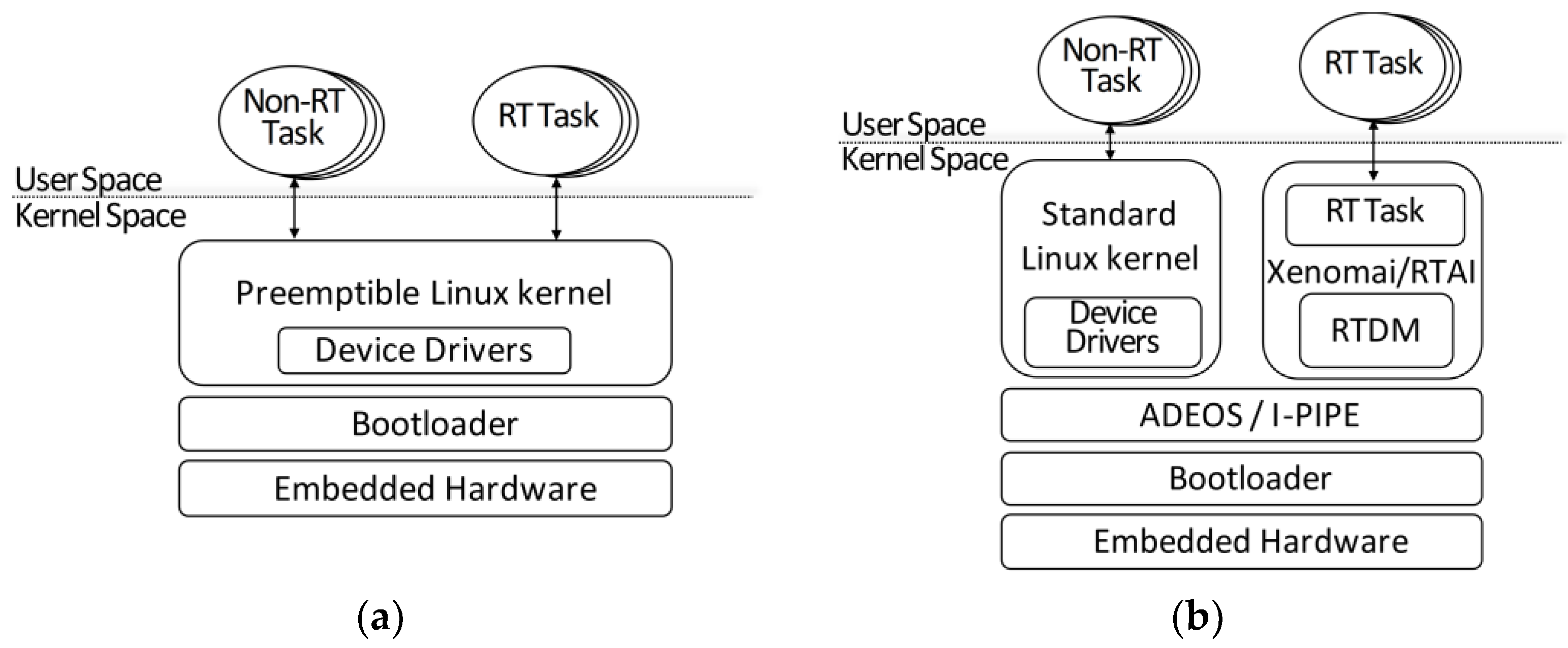
2.1. Real-Time Embedded Linux Approaches
2.2. Xenomai-Based Real-Time Environment
3. Performance Evaluation
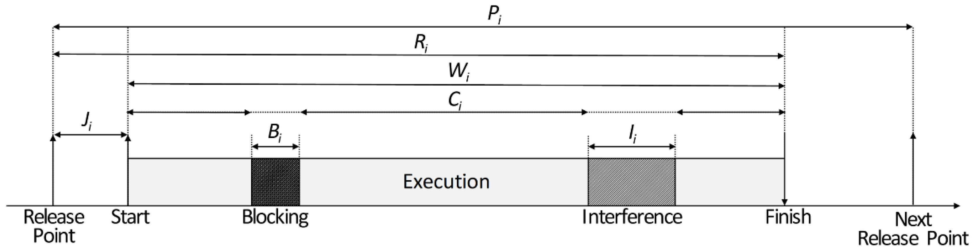
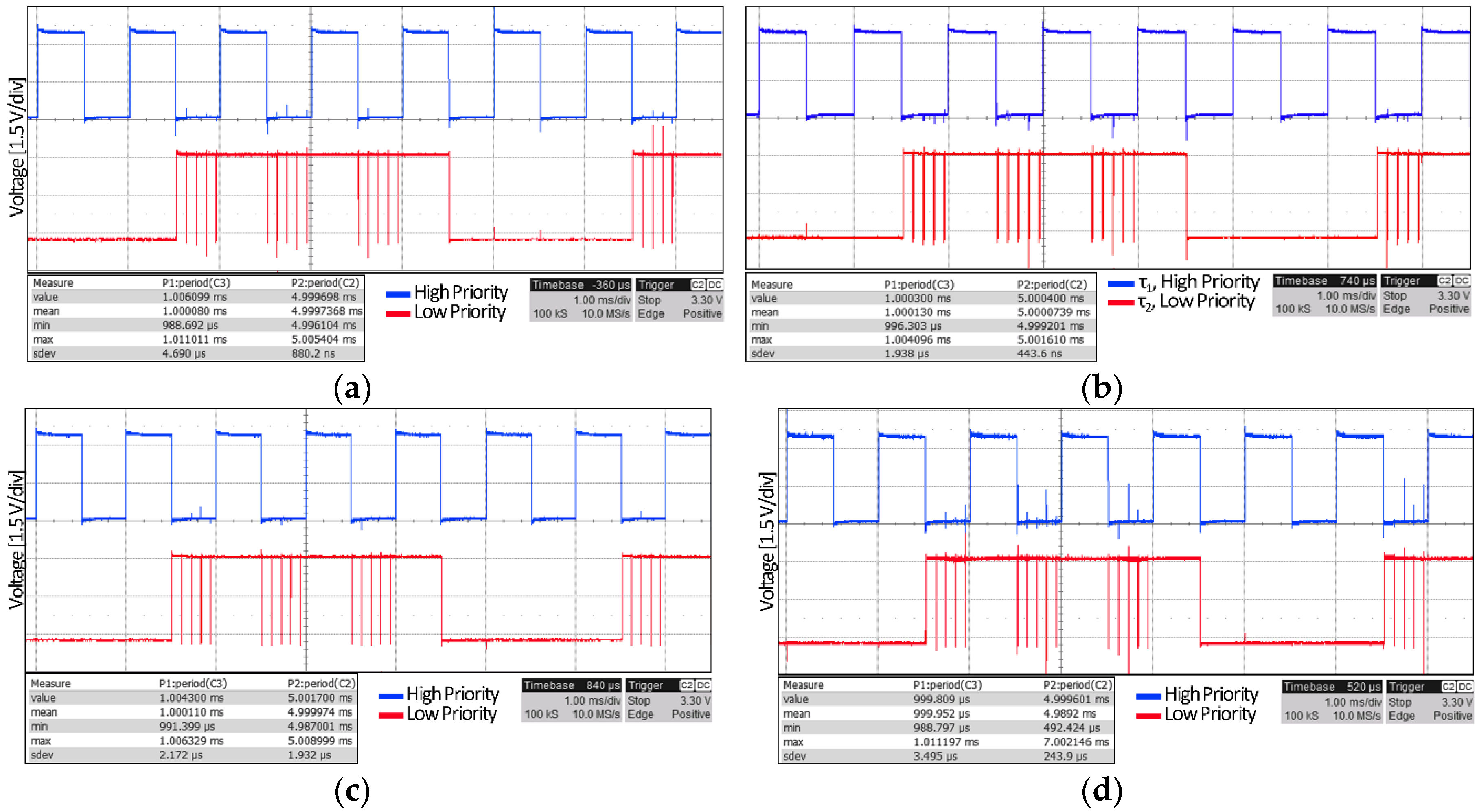
3.1. Periodicity and Responsiveness
3.2. Task Synchronization Mechanisms
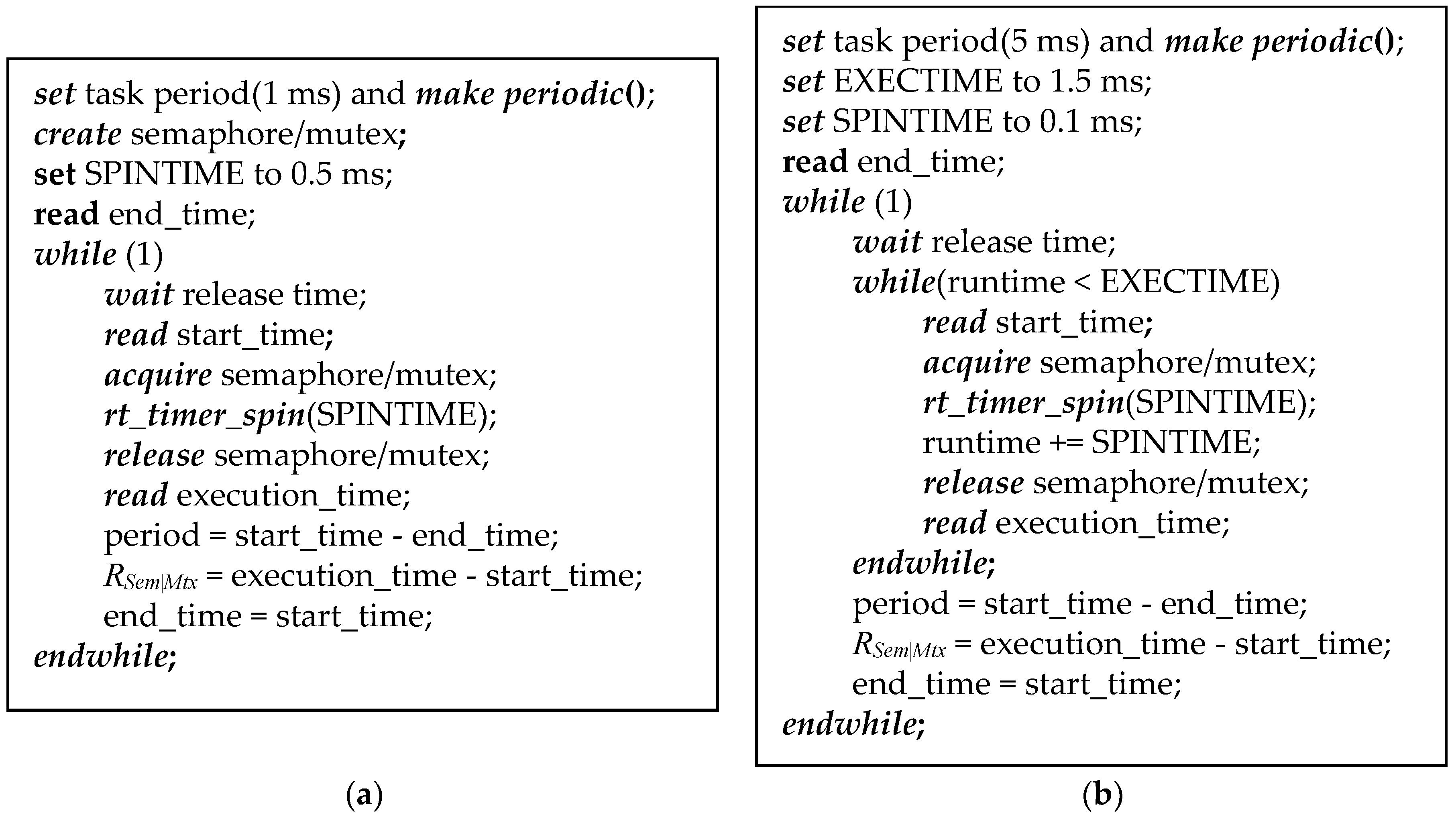
3.2.1. Semaphore and Mutex
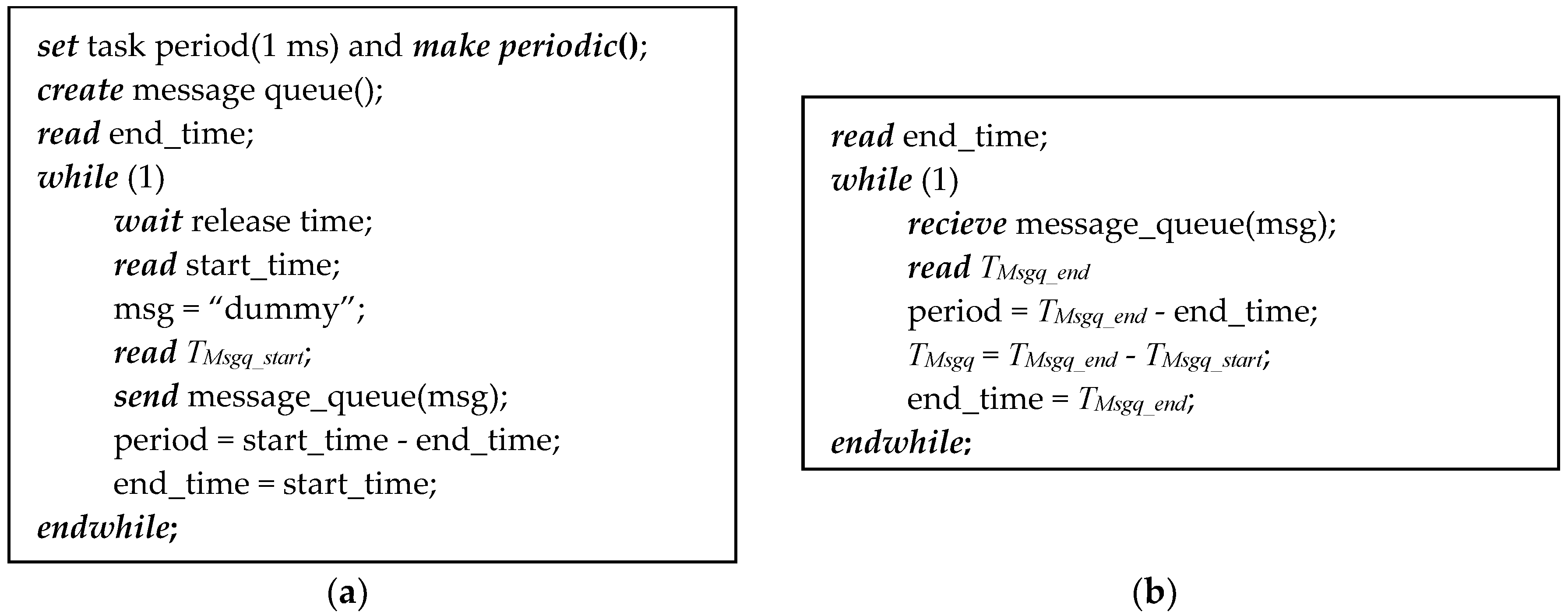
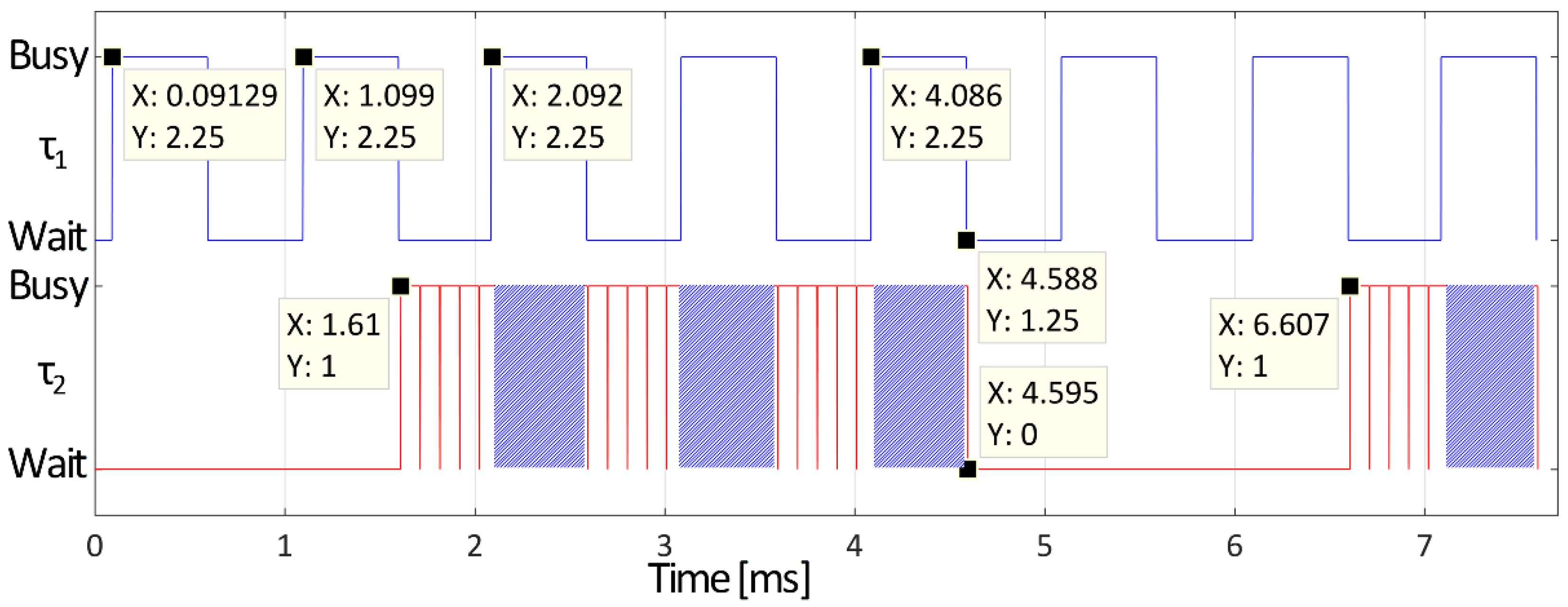
3.2.2. Message Queue
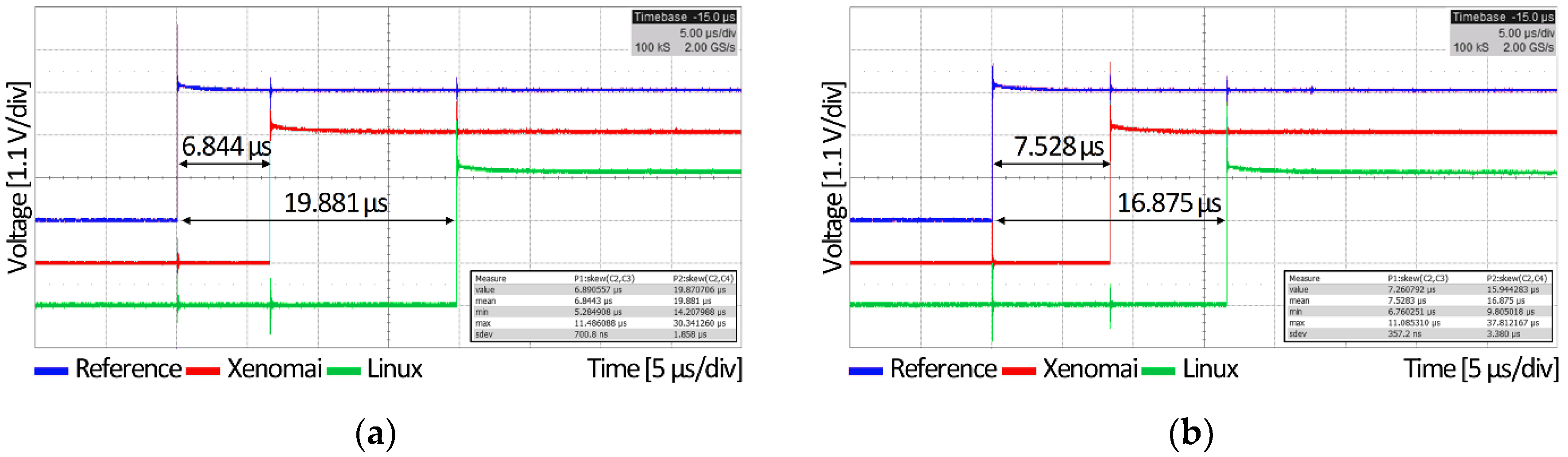
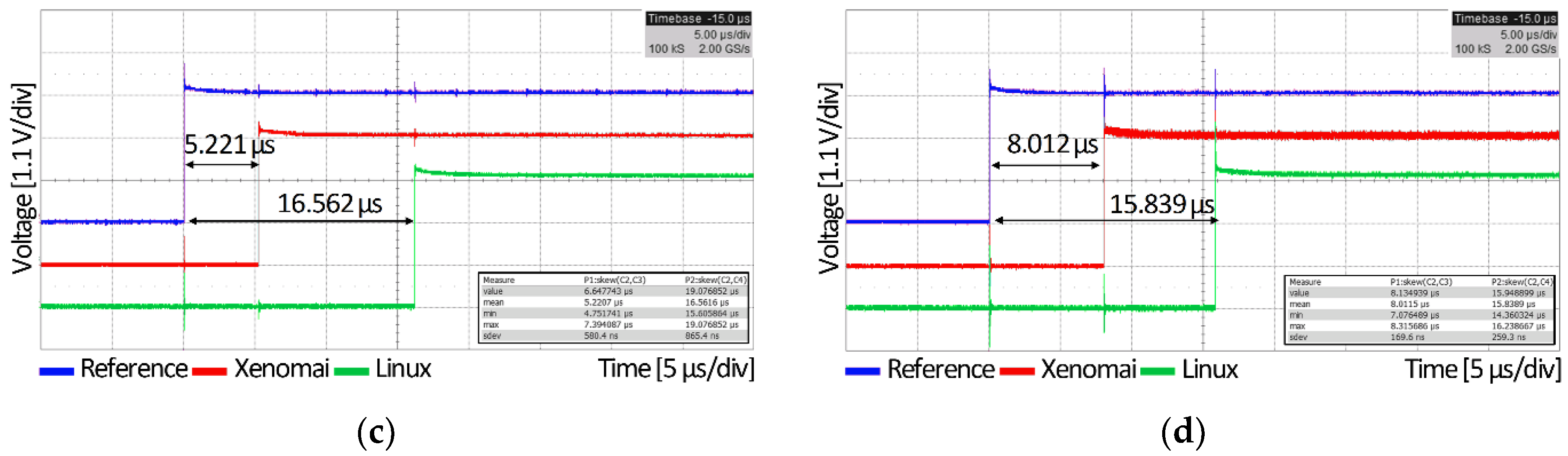
3.3. Interrupt Response Time
4. Example Cases Using OES as Real-time Controllers
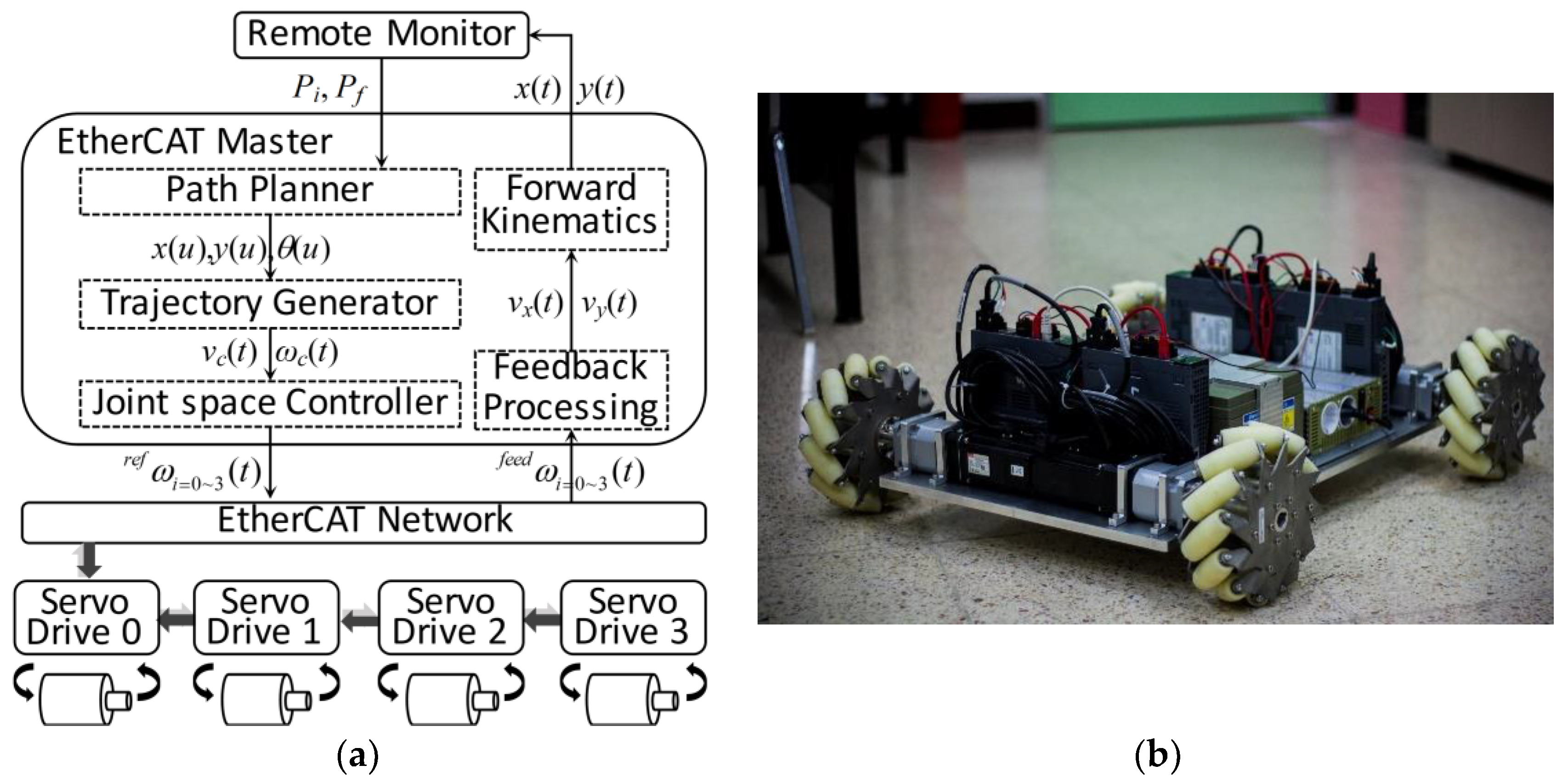
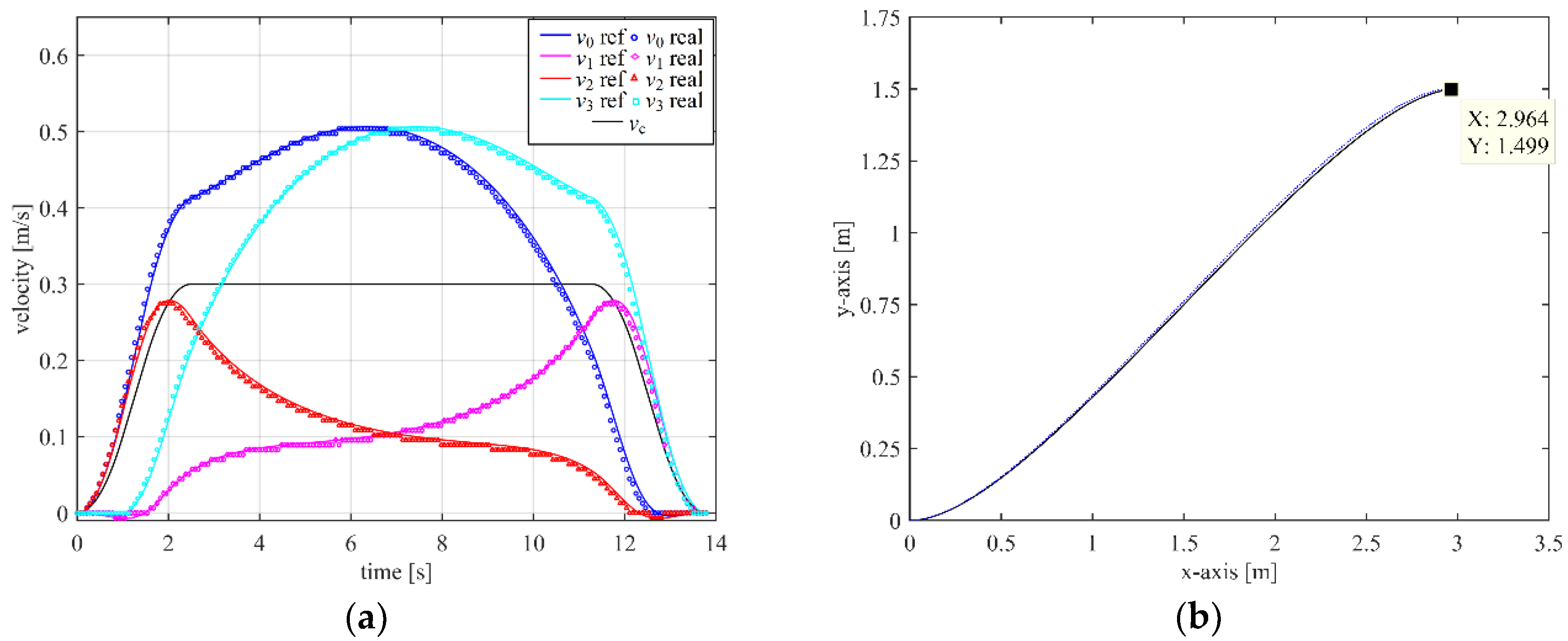
4.1. Real-Time Controller for Joint Space Motion of an Omnidirectional Mobile Robot
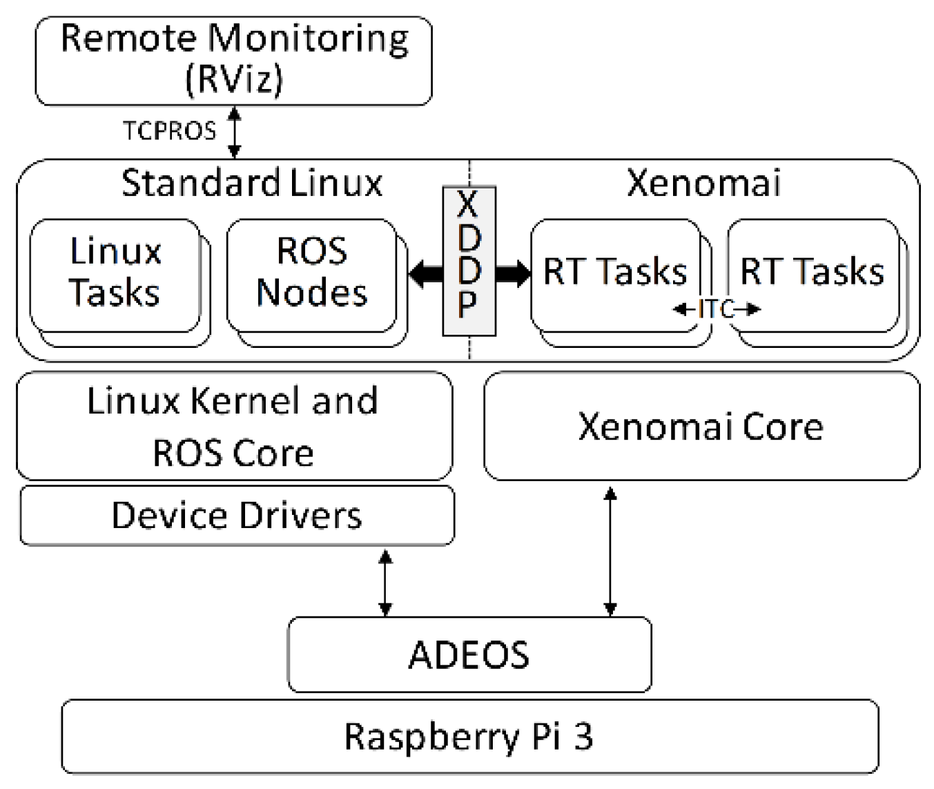
4.2. Integration of ROS in Real-Time Control Systems
5. Conclusions
Author Contributions
Funding
Acknowledgments
Conflicts of Interest
Appendix A
References
- Colnaric, M.; Verber, D.; Halang, W.A. Distributed Embedded Control Systems: Improving Dependability with Coherent Design; Springer Publishing Company: London, UK, 2008; p. 250. [Google Scholar]
- Brennan, R.W.; Fletcher, M.; Norrie, D.H. An agent-based approach to reconfiguration of real-time distributed control systems. IEEE Trans. Robot. Autom. 2002, 18, 444–451. [Google Scholar] [CrossRef]
- Omidvar, M.N.; Yang, M.; Mei, Y.; Li, X.; Yao, X. Dg2: A faster and more accurate differential grouping for large-scale black-box optimization. IEEE Trans. Evol. Comput. 2017, 21, 929–942. [Google Scholar] [CrossRef]
- Paschali, M.-E.; Ampatzoglou, A.; Bibi, S.; Chatzigeorgiou, A.; Stamelos, I. Reusability of open source software across domains: A case study. J. Syst. Softw. 2017, 134, 211–227. [Google Scholar] [CrossRef]
- Barbalace, A.; Luchetta, A.; Manduchi, G.; Moro, M.; Soppelsa, A.; Taliercio, C. Performance comparison of vxworks, linux, rtai, and xenomai in a hard real-time application. IEEE Trans. Nucl. Sci. 2008, 55, 435–439. [Google Scholar] [CrossRef]
- Abbott, D. Linux for Embedded and Real-Time Applications, 4th ed.; Butterworth-Heinemann: Newton, MA, USA, 2003; p. 250. [Google Scholar]
- Choi, B.W.; Shin, D.G.; Park, J.H.; Yi, S.Y.; Gerald, S. Real-time control architecture using xenomai for intelligent service robots in usn environments. Intell. Serv. Robot. 2009, 2, 139–151. [Google Scholar] [CrossRef]
- Oliveira, D.B.; Oliveira, R.S. Timing analysis of the preempt rt linux kernel. Softw. Pract. Exper. 2016, 46, 789–819. [Google Scholar] [CrossRef]
- Qian, K.Q.; Wang, J.; Gopaul, N.S.; Hu, B. Low cost multisensor kinematic positioning and navigation system with linux/rtai. J. Sens. Actuator Netw. 2012, 1, 166–182. [Google Scholar] [CrossRef]
- Yang, G.J.; Delgado, R.; Choi, B.W. A practical joint-space trajectory generation method based on convolution in real-time control. Int. J. Adv. Robot. Syst. 2016, 13, 56. [Google Scholar] [CrossRef]
- Dantam, N.T.; Lofaro, D.M.; Hereid, A.; Oh, P.Y.; Ames, A.D.; Stilman, M. The ach library: A new framework for real-time communication. IEEE Robot. Autom. Mag. 2015, 22, 76–85. [Google Scholar] [CrossRef]
- Cereia, M.; Bertolotti, I.C.; Scanzio, S. Performance of a real-time ethercat master under linux. IEEE Trans. Ind. Inform. 2011, 7, 679–687. [Google Scholar] [CrossRef]
- Jitendrasinh, T.B.; Deshpande, S. Implementation of can bus protocol on xenomai rtos on arm platform for industrial automation. In Proceedings of the 2016 International Conference on Computation of Power, Energy Information and Commuincation (ICCPEIC), Chennai, India, 20–21 April 2016; pp. 165–169. [Google Scholar]
- Kim, I.; Kim, T. Guaranteeing isochronous control of networked motion control systems using phase offset adjustment. Sensors 2015, 15, 13945–13965. [Google Scholar] [CrossRef] [PubMed]
- Brown, J.H.; Martin, B. How fast is fast enough? Choosing between Xenomai and Linux for real-time applications. In Proceedings of the 12th Real-Time Linux Workshop, Nairobi, Kenya, 25–27 October 2010; pp. 1–17. [Google Scholar]
- Ferdoush, S.; Li, X. Wireless sensor network system design using Raspberry Pi and Arduino for environmental monitoring applications. Procedia Comput. Sci. 2014, 34, 103–110. [Google Scholar] [CrossRef]
- Chianese, A.; Piccialli, F.; Riccio, G. Designing a smart multisensor framework based on beaglebone black board. In Lecture Notes in Electrical Engineering; Springer: Heidelberg, Germany, 2015; pp. 391–397. [Google Scholar]
- Honegger, D.; Meier, L.; Tanskanen, P.; Pollefeys, M. An open source and open hardware embedded metric optical flow cmos camera for indoor and outdoor applications. In Proceedings of the 2013 IEEE International Conference on Robotics and Automation, Karlsruhe, Germany, 6–10 May 2013; pp. 1736–1741. [Google Scholar]
- Kaliński, K.J.; Mazur, M. Optimal control at energy performance index of the mobile robots following dynamically created trajectories. Mechatronics 2016, 37, 79–88. [Google Scholar] [CrossRef]
- Zhang, L.; Slaets, P.; Bruyninckx, H. An open embedded hardware and software architecture applied to industrial robot control. In Proceedings of the 2012 IEEE International Conference on Mechatronics and Automation, Chengdu, China, 5–8 August 2012; pp. 1822–1828. [Google Scholar]
- Su, Y.; Qiu, Y.; Liu, P. The continuity and real-time performance of the cable tension determining for a suspend cable-driven parallel camera robot. Adv. Robot. 2015, 29, 743–752. [Google Scholar] [CrossRef]
- Arm, J.; Bradac, Z.; Kaczmarczyk, V. Real-time capabilities of linux rtai. IFAC-PapersOnLine 2016, 49, 401–406. [Google Scholar] [CrossRef]
- Kiszka, J. The real-time driver model and first applications. In Proceedings of the 7th Real-Time Linux Workshop, Lille, France, 2–4 November 2005; pp. 1–8. [Google Scholar]
- Xenomai Archives. Available online: http://xenomai.org/downloads/xenomai/stable (accessed on 10 November 2018).
- Beaglebone Black Linux Kernel. Available online: https://github.com/RobertCNelson/bb-kernel (accessed on 17 November 2018).
- Raspberry pi 3 Linux Kernel. Available online: https://github.com/raspberrypi/linux (accessed on 22 November 2018).
- Zybo-7020 Linux Kernel. Available online: https://github.com/Xilinx/linux-xlnx (accessed on 25 November 2018).
- MX6Q SABRELite Linux Kernel. Available online: https://github.com/RobertCNelson/armv7-multiplatform (accessed on 25 November 2018).
- Pipe Patch Archives. Available online: https://xenomai.org/downloads/ipipe/v3.x/arm/older (accessed on 10 November 2018).
- Raspberry pi 3 Image Repository. Available online: http://downloads.raspberrypi.org/raspbian_lite/images/raspbian_lite-2017-07-05 (accessed on 22 November 2018).
- U-Boot Bootloader. Available online: http://git.denx.de (accessed on 10 November 2018).
- Pose, F. Igh Ethercat Master 1.5.2 Documentation. Available online: https://www.etherlab.org/download/ethercat/ethercat-1.5.2.pdf (accessed on 27 November 2018).
- Minimal Ubuntu 14.04. Available online: https://rcn-ee.com/rootfs/eewiki/minfs (accessed on 11 November 2018).
- Delgado, R.; Hong, C.H.; Shin, W.C.; Choi, B.W. Implementation and perfomance analysis of an Ethercat master on the latest real-time embedded Linux. Int. J. Appl. Eng. Res. 2015, 10, 44603–44609. [Google Scholar]
- Joseph, M.; Pandya, P. Finding response times in a real-time system. Comput. J. 1986, 29, 390–395. [Google Scholar] [CrossRef]
- Harbour, M.G.; Garcia, J.J.G.; Gutierrez, J.C.P.; Moyano, J.M.D. Mast: Modeling and analysis suite for real time applications. In Proceedings of the 13th Euromicro Conference on Real-Time Systems, Delft, The Netherlands, 13–15 June 2001; pp. 125–134. [Google Scholar]
- Delgado, R.; Shin, W.C.; Hong, C.H.; Choi, B.W. Development and control of an omnidirectional mobile robot on an ethercat network. Int. J. Appl. Eng. Res. 2016, 11, 10586–10592. [Google Scholar]
- Delgado, R.; You, B.-J.; Choi, B.W. Real-time control architecture based on xenomai using ros packages for a service robot. J. Syst. Softw. 2019, 151, 8–19. [Google Scholar] [CrossRef]
- Delgado, R.; You, B.-J.; Han, M.; Choi, B.W. Integration of ros and rt tasks using message pipe mechanism on xenomai for telepresence robot. Electron. Lett. 2019, 55, 127–128. [Google Scholar] [CrossRef]
- Mamun, M.A.A.; Nasir, M.T.; Khayyat, A. Embedded system for motion control of an omnidirectional mobile robot. IEEE Access 2018, 6, 6722–6739. [Google Scholar] [CrossRef]
- Arvin, F.; Espinosa, J.; Bird, B.; West, A.; Watson, S.; Lennox, B. Mona: An affordable open-source mobile robot for education and research. J. Intell. Robot. Syst. 2018, 1–15. [Google Scholar] [CrossRef]
- López-Rodríguez, F.M.; Cuesta, F. Andruino-a1: Low-cost educational mobile robot based on android and arduino. J. Intell. Robot. Syst. 2016, 81, 63–76. [Google Scholar] [CrossRef]
- You, B.-J.; Kwon, J.R.; Nam, S.-H.; Lee, J.-J.; Lee, K.-K.; Yeom, K. Coexistent space: Toward seamless integration of real, virtual, and remote worlds for 4D+ interpersonal interaction and collaboration. In Proceedings of the SIGGRAPH Asia 2014 Autonomous Virtual Humans and Social Robot for Telepresence, Shenzhen, China, 3–6 December 2014; pp. 1–5. [Google Scholar]


| Software Component | BeagleBone Black | Raspberry Pi 3 | Zybo-7020 | i.MX6Q SABRELite |
|---|---|---|---|---|
| Toolchain | gcc-linaro-arm-linux-gnueabihf-4.7.3 | gcc-linaro-arm-linux-gnueabihf-raspbian-4.8.3 | gcc-linaro-arm-linux-gnueabihf-4.8.3 | gcc-linaro-arm-linux-gnueabihf-4.8.3 |
| Bootloader | U-Boot 2015.10 | Broadcom Bootloader | U-Boot 2015.10 | U-Boot 2015.10 |
| ADEOS/I-PIPE | ipipe-3.8.13-arm-3 | ipipe-4.1.18-arm-4 | ipipe-3.14.17-arm-4 | ipipe-3.14.17-arm-2 |
| Xenomai | 2.6.5 [24] | 3.0.2 [24] | 2.6.5 | 2.6.5 |
| Linux Kernel | 3.8.13 [25] | 4.1.21 [26] | 3.14.2 [27] | 3.14.15 [28] |
| Root Filesystem | Minimal Ubuntu 14.04 | Raspbian Jessie | Minimal Ubuntu 14.04 | Minimal Ubuntu 14.04 |
| IgH EtherCAT | 1.5.2 | - | 1.5.2 | 1.5.2 |
| Task | Priority | Worst-Case Response (ms) | Slack (%) |
|---|---|---|---|
| τ1 | 99 | 0.500000 | 39.45% |
| τ2 | 80 | 3.000000 | 65.63% |
| Task | τ1, High Priority (99, 1 ms Deadline) | τ2, Low Priority (80, 5 ms Deadline) | ||||
|---|---|---|---|---|---|---|
| Metric (ms) | Period (P) | Response (R) | Jitter (J) | Period (P) | Response (R) | Jitter (J) |
| BeagleBone Black | ||||||
| avg. | 1.000000 | 0.502764 | 0.004424 | 5.000000 | 2.987725 | 0.001938 |
| max. | 1.029958 | 0.510792 | 0.029958 | 5.028000 | 3.001875 | 0.028000 |
| min. | 0.972792 | 0.502125 | 0.000000 | 4.976250 | 2.963000 | 0.000000 |
| st.d (σ) | 0.006238 | 0.000667 | 0.004398 | 0.003521 | 0.004687 | 0.002940 |
| Raspberry Pi 3 | ||||||
| avg. | 1.000000 | 0.500780 | 0.001121 | 5.000000 | 2.994471 | 0.000617 |
| max. | 1.007084 | 0.503437 | 0.008906 | 5.008959 | 2.998542 | 0.008959 |
| min. | 0.991094 | 0.500520 | 0.000000 | 4.993646 | 2.989844 | 0.000000 |
| st.d (σ) | 0.001429 | 0.000164 | 0.001124 | 0.000951 | 0.000666 | 0.000723 |
| Zybo-7020 | ||||||
| avg. | 1.000000 | 0.502655 | 0.000878 | 5.000000 | 2.998630 | 0.001120 |
| max. | 1.010889 | 0.509745 | 0.010909 | 5.015211 | 3.003186 | 0.015323 |
| min. | 0.989091 | 0.502341 | 0.000000 | 4.984677 | 2.984868 | 0.000001 |
| st.d (σ) | 0.001588 | 0.000332 | 0.001127 | 0.002187 | 0.002377 | 0.001878 |
| i.MX6Q SABRELite | ||||||
| avg. | 1.000000 | 0.502450 | 0.001423 | 5.000000 | 2.996607 | 0.003339 |
| max. | 1.010803 | 0.508783 | 0.012045 | 5.015409 | 3.002187 | 0.015409 |
| min. | 0.987955 | 0.501965 | 0.000000 | 4.987518 | 2.984358 | 0.000000 |
| st.d (σ) | 0.002163 | 0.000913 | 0.001629 | 0.004488 | 0.003698 | 0.002999 |
| Mechanism | Semaphore | Mutex | ||
|---|---|---|---|---|
| avg. (μs) | RSem | TSem | RMtx | TMtx |
| BeagleBone Black | 531.52 | 28.756 | 532.090 | 29.326 |
| Raspberry Pi 3 | 527.443 | 26.663 | 531.018 | 30.238 |
| Zybo-7020 | 533.255 | 30.6 | 534.376 | 31.721 |
| i.MX6Q SABRELite | 537.04 | 34.59 | 542.864 | 40.414 |
| Mechanism | Message Queue | ||
|---|---|---|---|
| Metric | P,τ1 (ms) | P,τ2 (ms) | TMsgq (μs) |
| BeagleBone Black | |||
| avg. | 1.000000 | 1.000000 | 18.748 |
| max. | 1.036625 | 1.059042 | 41.459 |
| min. | 0.976375 | 0.961084 | 14.375 |
| st.d (σ) | 0.002621 | 0.004464 | 3.805 |
| Raspberry Pi 3 | |||
| avg. | 1.000000 | 1.000000 | 15.341 |
| max. | 1.005989 | 1.015000 | 24.531 |
| min. | 0.994532 | 0.986979 | 14.740 |
| st.d (σ) | 0.000522 | 0.000609 | 0.224 |
| Zybo-7020 | |||
| avg. | 1.000000 | 1.000000 | 14.627 |
| max. | 1.012644 | 1.029186 | 31.596 |
| min. | 0.985410 | 0.968832 | 11.454 |
| st.d (σ) | 0.000939 | 0.002162 | 0.789 |
| i.MX6Q SABRELite | |||
| avg. | 1.000000 | 1.000000 | 14.376 |
| max. | 1.009421 | 1.013699 | 24.722 |
| min. | 0.991685 | 0.985530 | 9.898 |
| st.d (σ) | 0.001676 | 0.002172 | 0.498 |
| Task | Period (ms) | Execution (ms) | Priority | Worst-Case Response (ms) | Slack (%) |
|---|---|---|---|---|---|
| Actuator | 10.000 | 0.029 | 99 | 0.029 | 31,082.4% |
| IMU | 10.000 | 0.432 | 95 | 0.461 | 2086.3% |
| LED | 20.000 | 0.590 | 90 | 1.051 | 3055.5% |
| Sonar | 30.000 | 0.460 | 85 | 1.511 | 5864.5% |
| LRF | 200.000 | 0.762 | 80 | 2.273 | 23,694.1% |
© 2019 by the authors. Licensee MDPI, Basel, Switzerland. This article is an open access article distributed under the terms and conditions of the Creative Commons Attribution (CC BY) license (http://creativecommons.org/licenses/by/4.0/).
Share and Cite
Delgado, R.; Park, J.; Choi, B.W. Open Embedded Real-time Controllers for Industrial Distributed Control Systems. Electronics 2019, 8, 223. https://doi.org/10.3390/electronics8020223
Delgado R, Park J, Choi BW. Open Embedded Real-time Controllers for Industrial Distributed Control Systems. Electronics. 2019; 8(2):223. https://doi.org/10.3390/electronics8020223
Chicago/Turabian StyleDelgado, Raimarius, Jaeho Park, and Byoung Wook Choi. 2019. "Open Embedded Real-time Controllers for Industrial Distributed Control Systems" Electronics 8, no. 2: 223. https://doi.org/10.3390/electronics8020223
APA StyleDelgado, R., Park, J., & Choi, B. W. (2019). Open Embedded Real-time Controllers for Industrial Distributed Control Systems. Electronics, 8(2), 223. https://doi.org/10.3390/electronics8020223