Vehicle Sideslip Angle Estimation Based on Tire Model Adaptation


Abstract
:1. Introduction
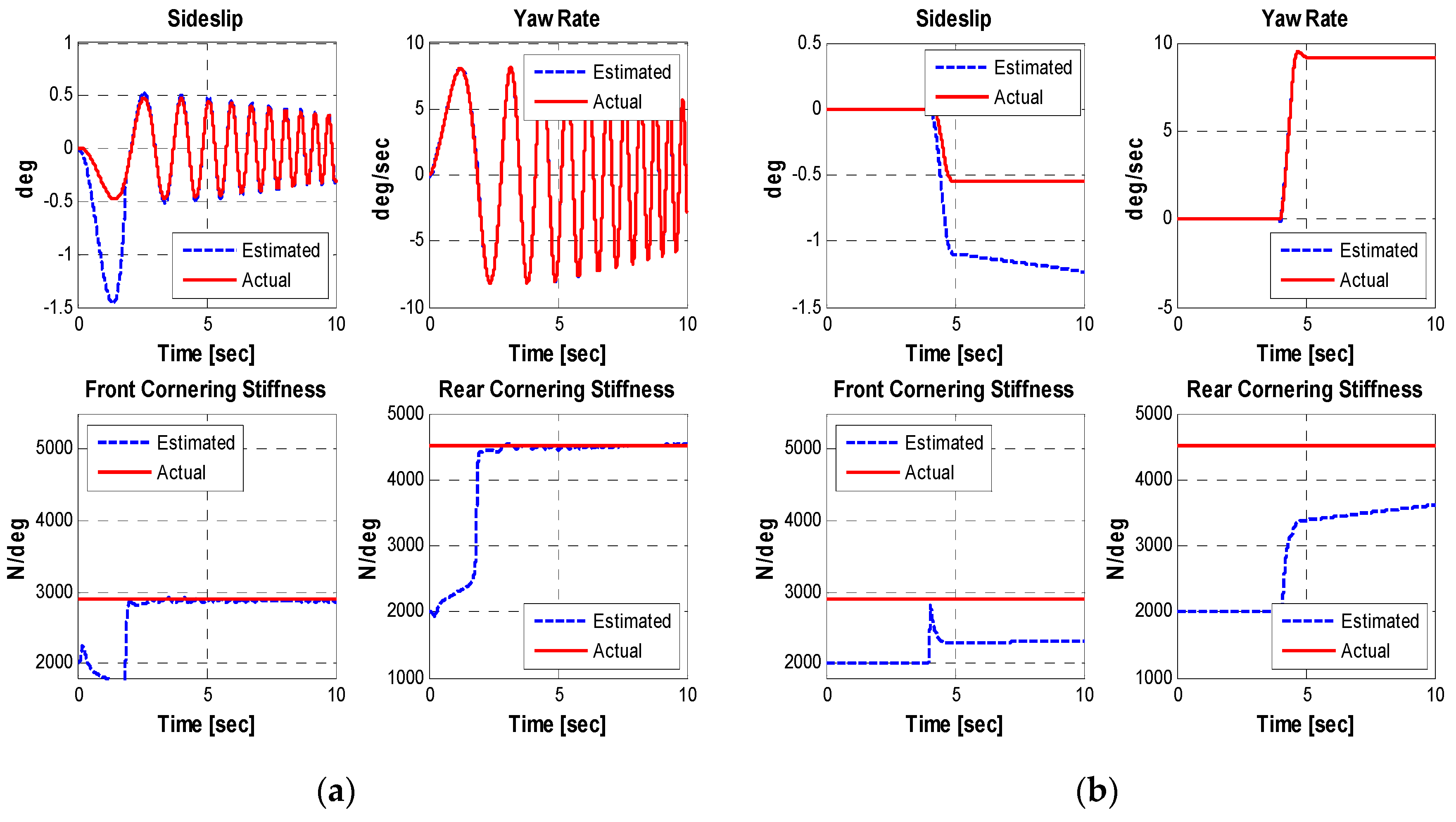
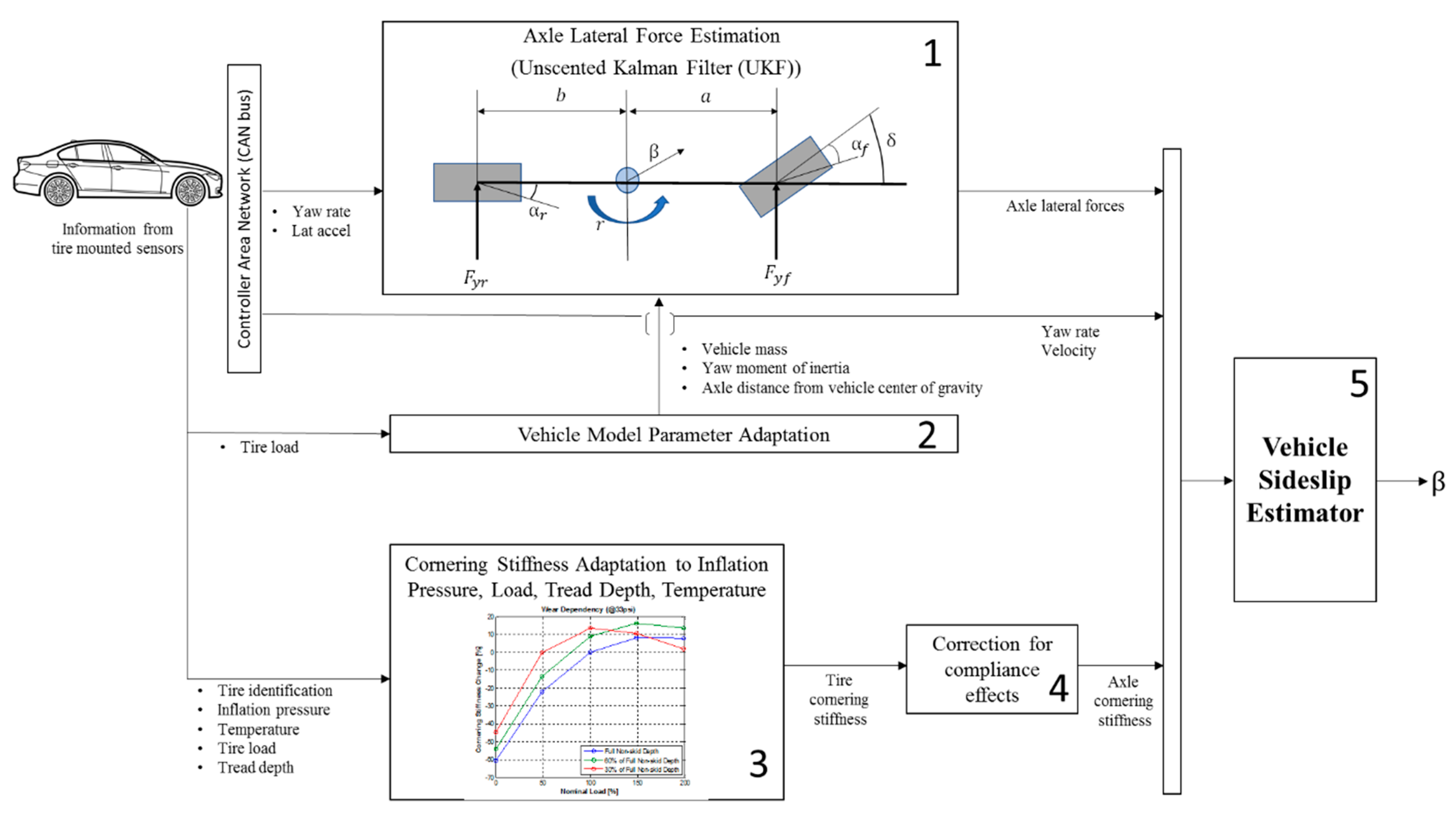
- The state vector, at each time instant k comprises of sideslip angle, yaw rate, front tire cornering stiffness and rear tire cornering stiffness.
- The measurement vector comprises of yaw rate and front and rear axle lateral forces.
- Accurate knowledge of the tire cornering stiffness is crucial for ensuring good estimates of vehicle sideslip angle using model-based observers.
- Observers for cornering stiffness estimation do not give satisfactory estimates during steady state maneuvers.
- The availability of a high-fidelity cornering stiffness model would facilitate the online computation of the vehicle sideslip angle.
- Tires have a service life and get changed on a vehicle every few years. There is no way for the vehicle to know the properties of the new tire purchased by the customer.
- Customers in European countries typically have different tires mounted based on the season (summer or winter), mainly due to government mandated requirements. Tires built with different rubber compounds and structural properties (e.g. summer versus winter tires) behave very differently.
- During its normal service life, a tire is subjected to large variations in operating conditions such as ambient temperature, inflation pressure and changes in tread depth. The force and moment characteristics of the tire changes significantly due to each of these operating conditions.
- Quantification of influence of operating conditions on tire cornering stiffness.
- Extension of cornering stiffness expression for Pacejka’s Magic Formula to inflation pressure, temperature, load and tread depth.
- A novel framework for estimating vehicle sideslip angle.
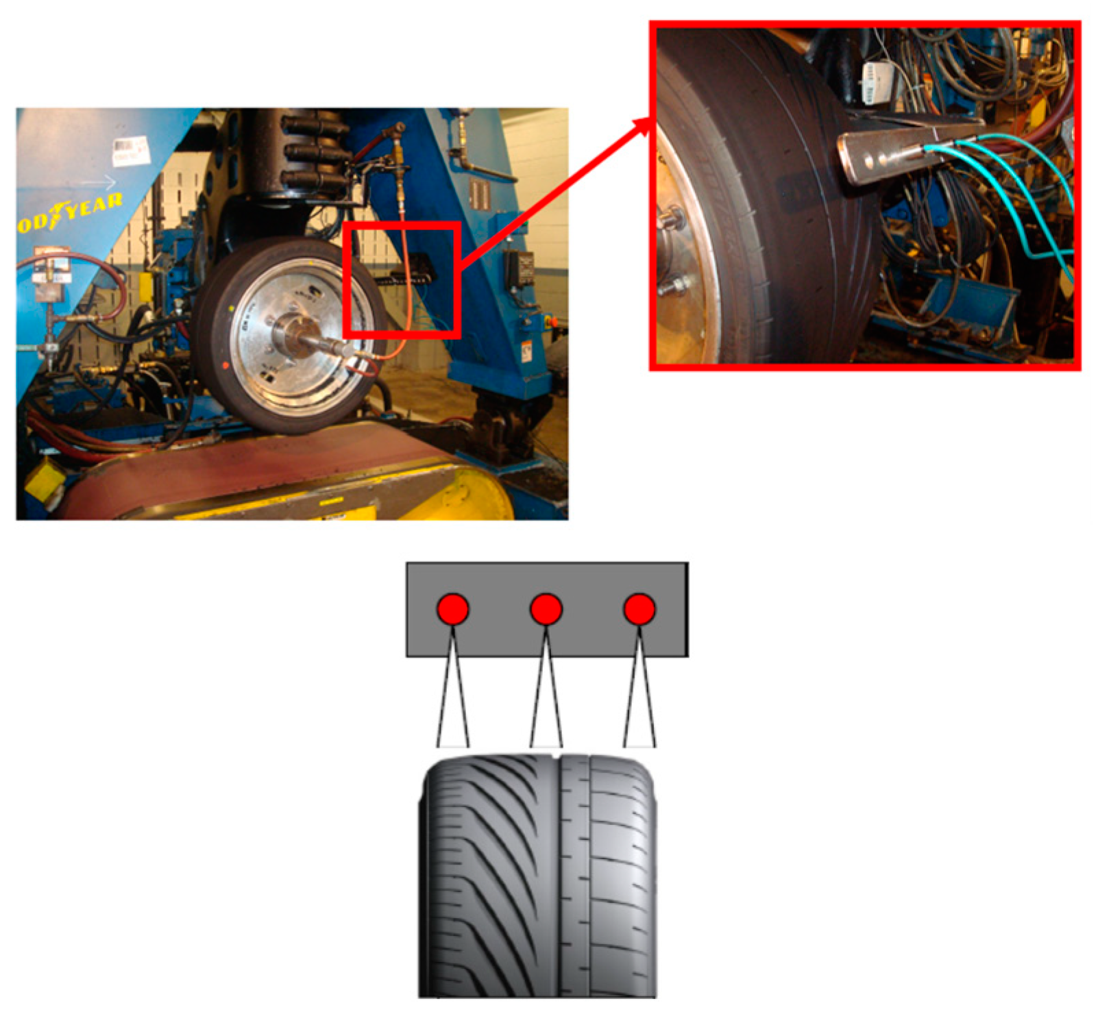
2. Quantifying the Influence of Variations in the Tire Inflation Pressure, Tread Depth, Load and Temperature on the Tire Cornering Stiffness
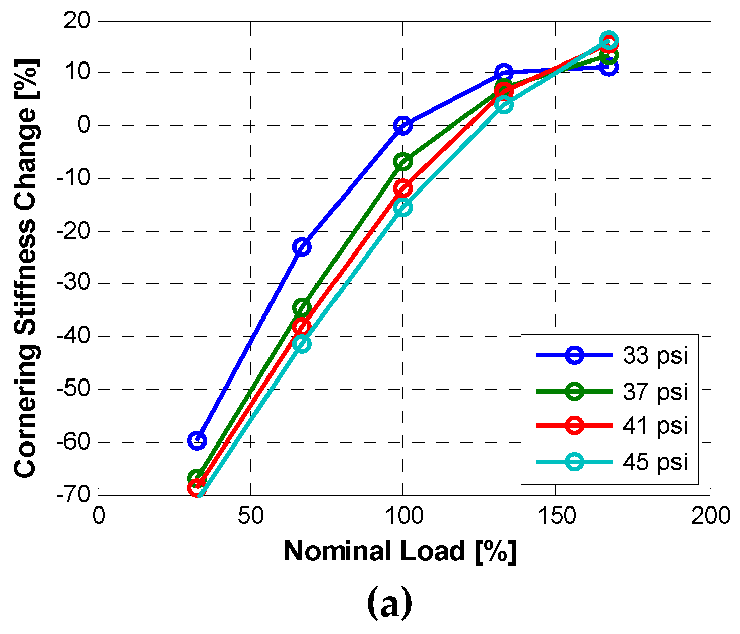
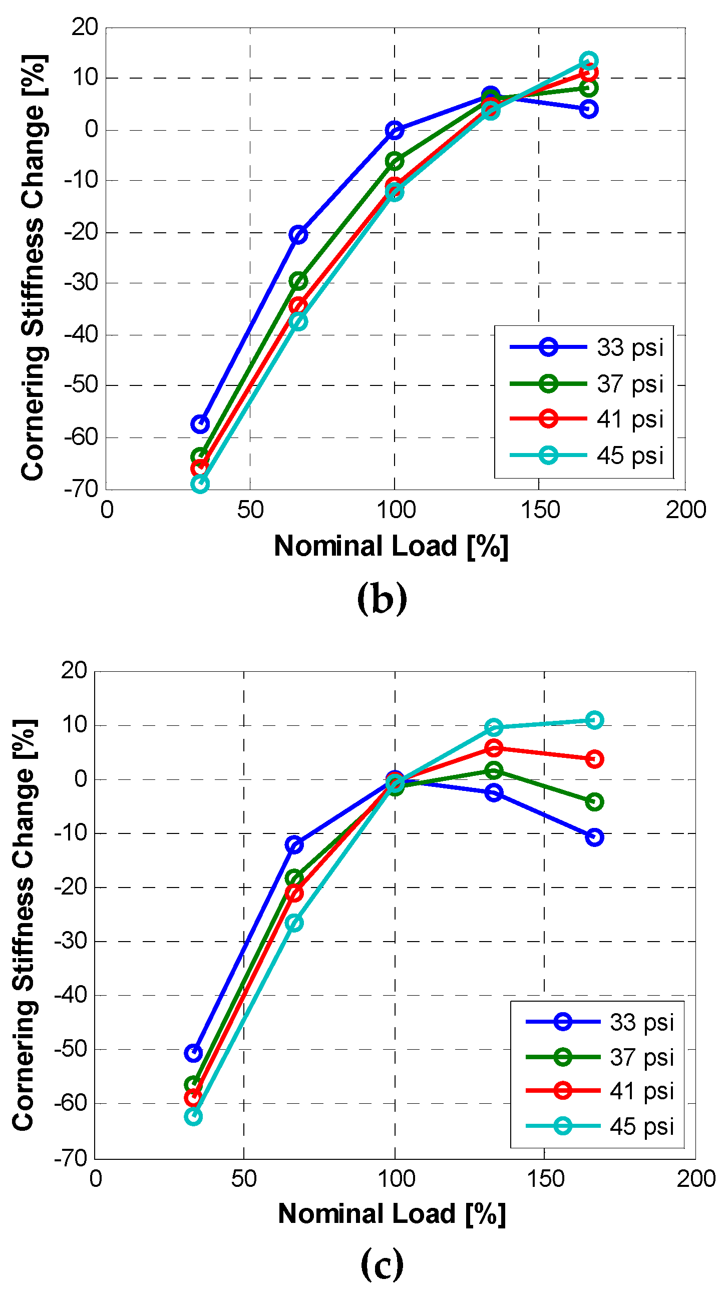
- To evaluate the influence of the inflation pressure on the tire characteristics, four levels of pressure were analyzed: (a) 33 psi, (b) 37 psi, (c) 41 psi and (d) 45 psi.
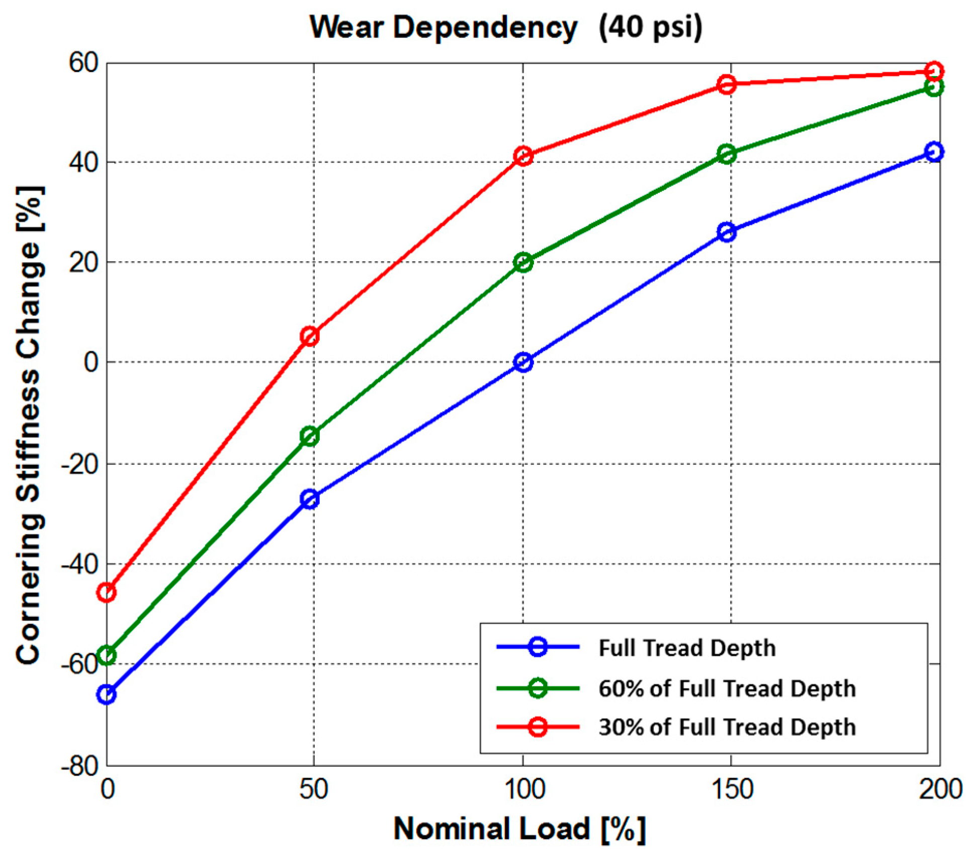
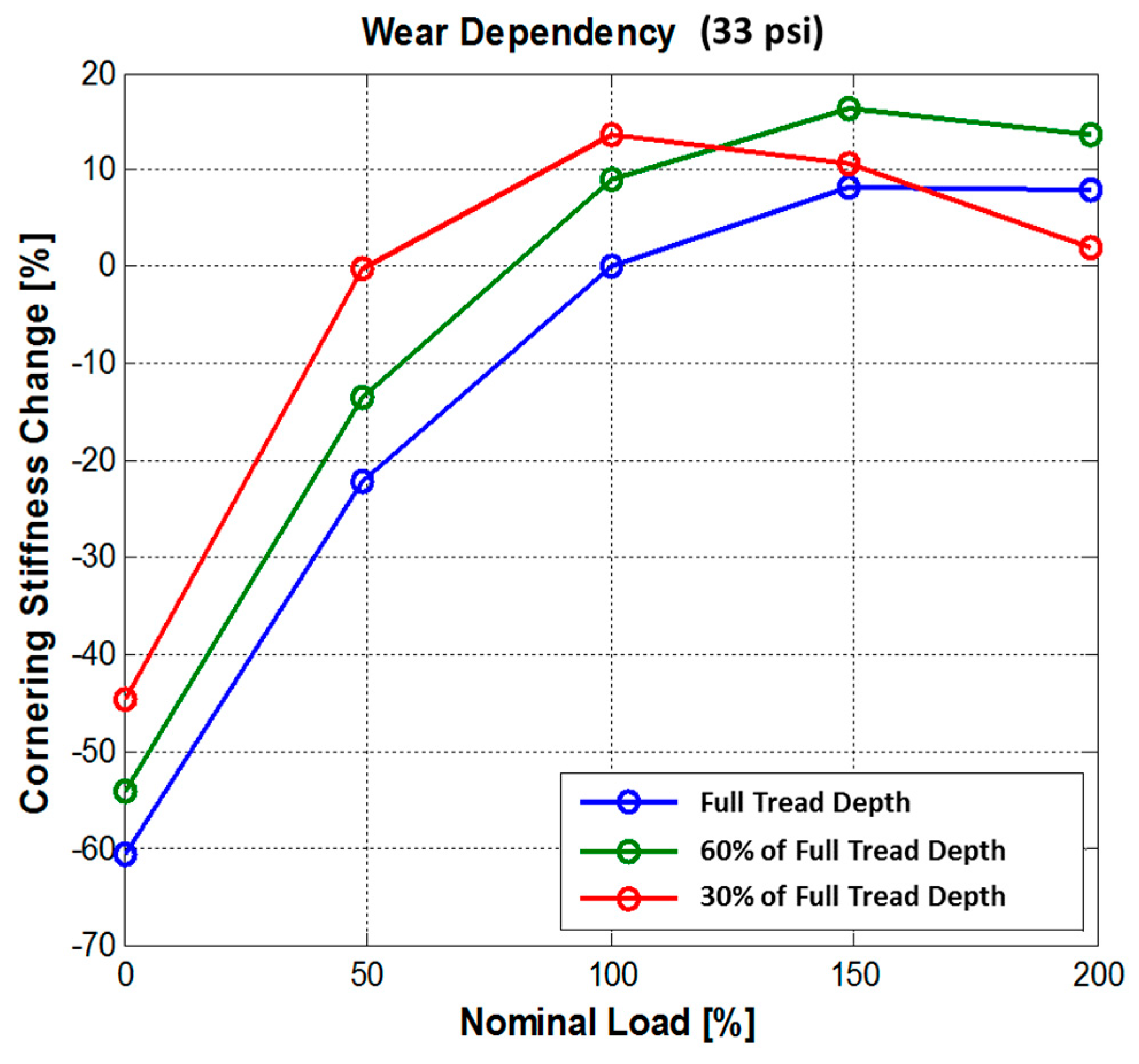
- To evaluate the influence of the tire tread depth on the tire characteristics, three levels of tread depth were analyzed: (a) full tread depth, (b) 60% of full tread depth and (c) 30% of full tread depth.
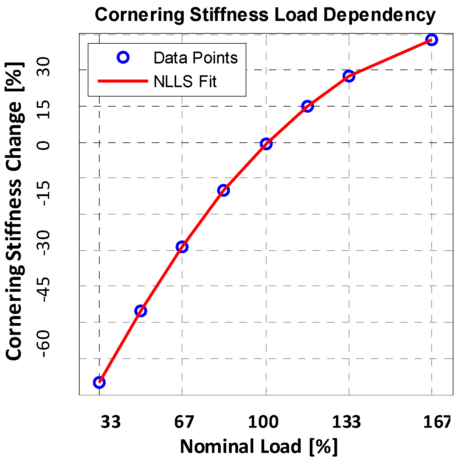
- To evaluate the influence of the tire load on the tire characteristics, five levels of normal load were analyzed: (a) 33% of nominal load, (b) 67% of nominal load, (c) 100% of nominal load. (d) 133% of nominal load and (e) 167% of nominal load.
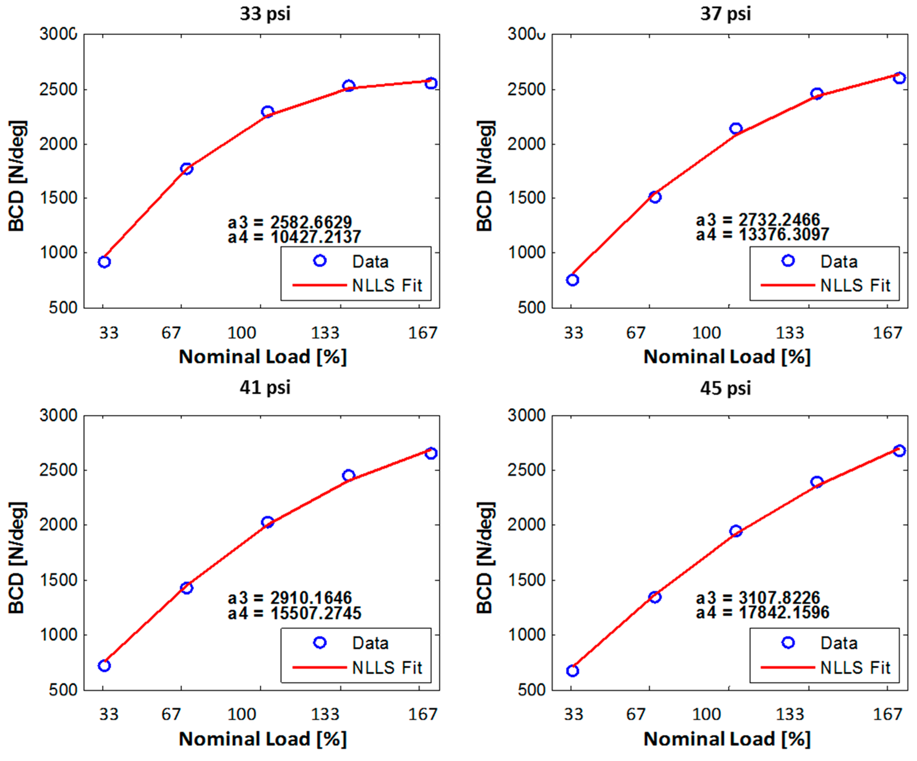
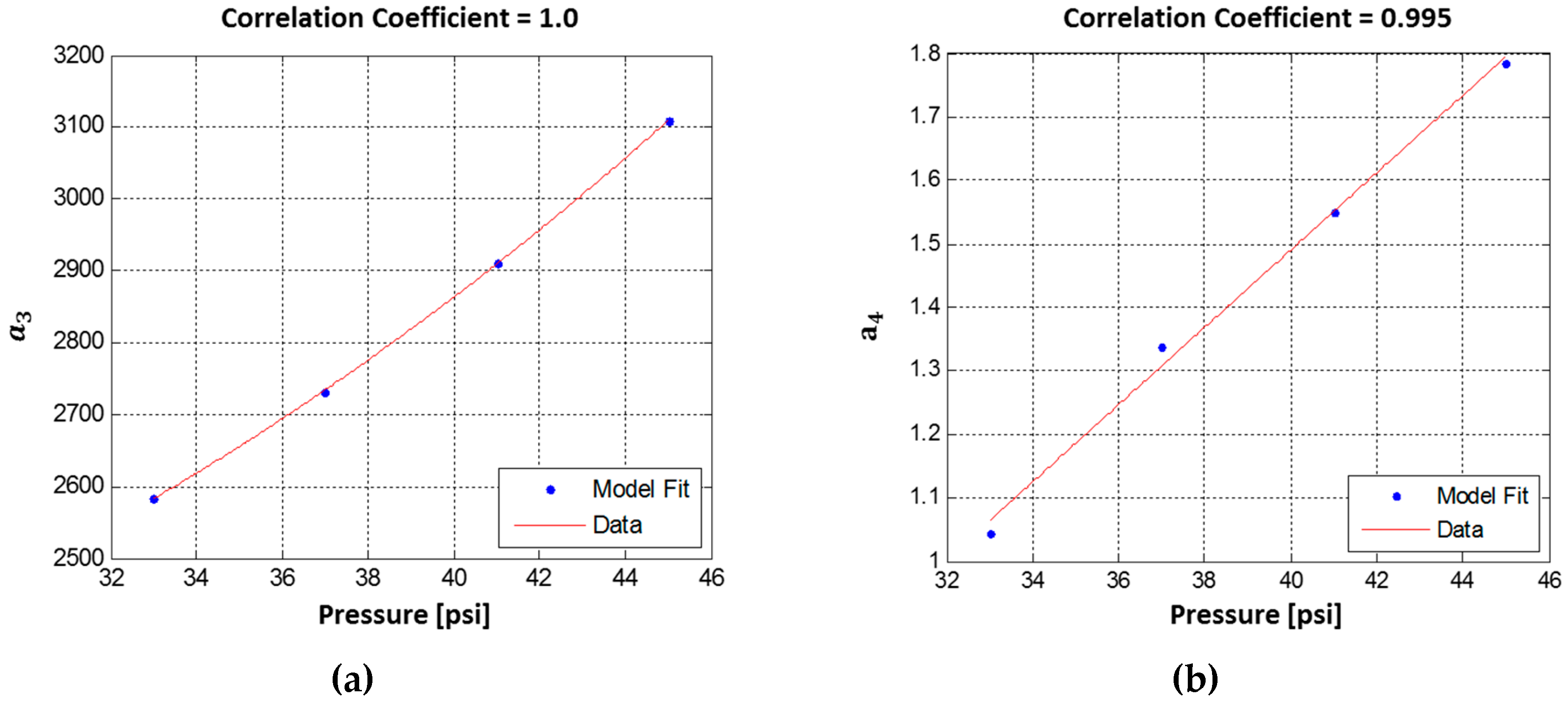
2.1. Influence of Inflation Pressure
- A lower cornering stiffness at low vertical loads and a higher cornering stiffness at high vertical loads. These effects are clearly visible in Figure 9. The first effect is caused by the decreasing contact length because of the increased vertical stiffness from the increased inflation. A decrease of contact length (smaller surface area) results in a decrease of cornering stiffness. In the range of high vertical loads, this effect may also be present, but it is not dominant.
- A lower inflation pressure, and consequently a less stiff carcass, results in more rotation of the contact patch. This leads to lower lateral force for the same slip angle, which results in a lower cornering stiffness at high vertical loads. Conversely, a higher inflation pressure, and consequently a stiffer carcass, results in less rotation of the contact patch. This leads to higher lateral force for the same slip angle, which results in a higher cornering stiffness at high vertical loads.
2.2. Influence of Tread Depth
- Lower tread depth results in a higher cornering stiffness.
- At higher loads, carcass stiffness is the dominant component of cornering stiffness. Hence, even a large change in the tread depth only results in a smaller change in the cornering stiffness.
- For a tire with a lower tread depth, the cornering stiffness properties are dominated by the carcass stiffness characteristics.
- As explained previously, lowering the tire inflation pressure decreases the carcass stiffness, which explains the saturation trends seen in the CS curve.
- Furthermore, the saturation starts even earlier for a tire with a lower tread depth due to the dominant effect of carcass stiffness.
2.3. Influence of Normal Load
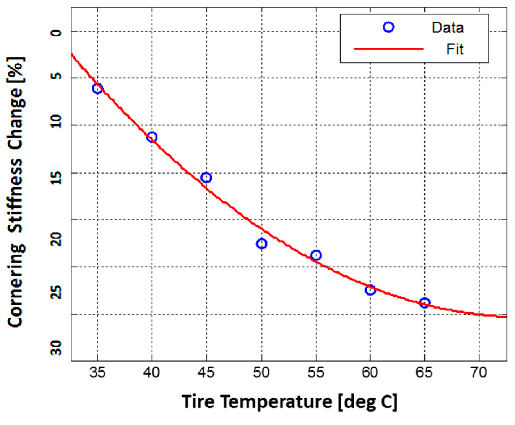
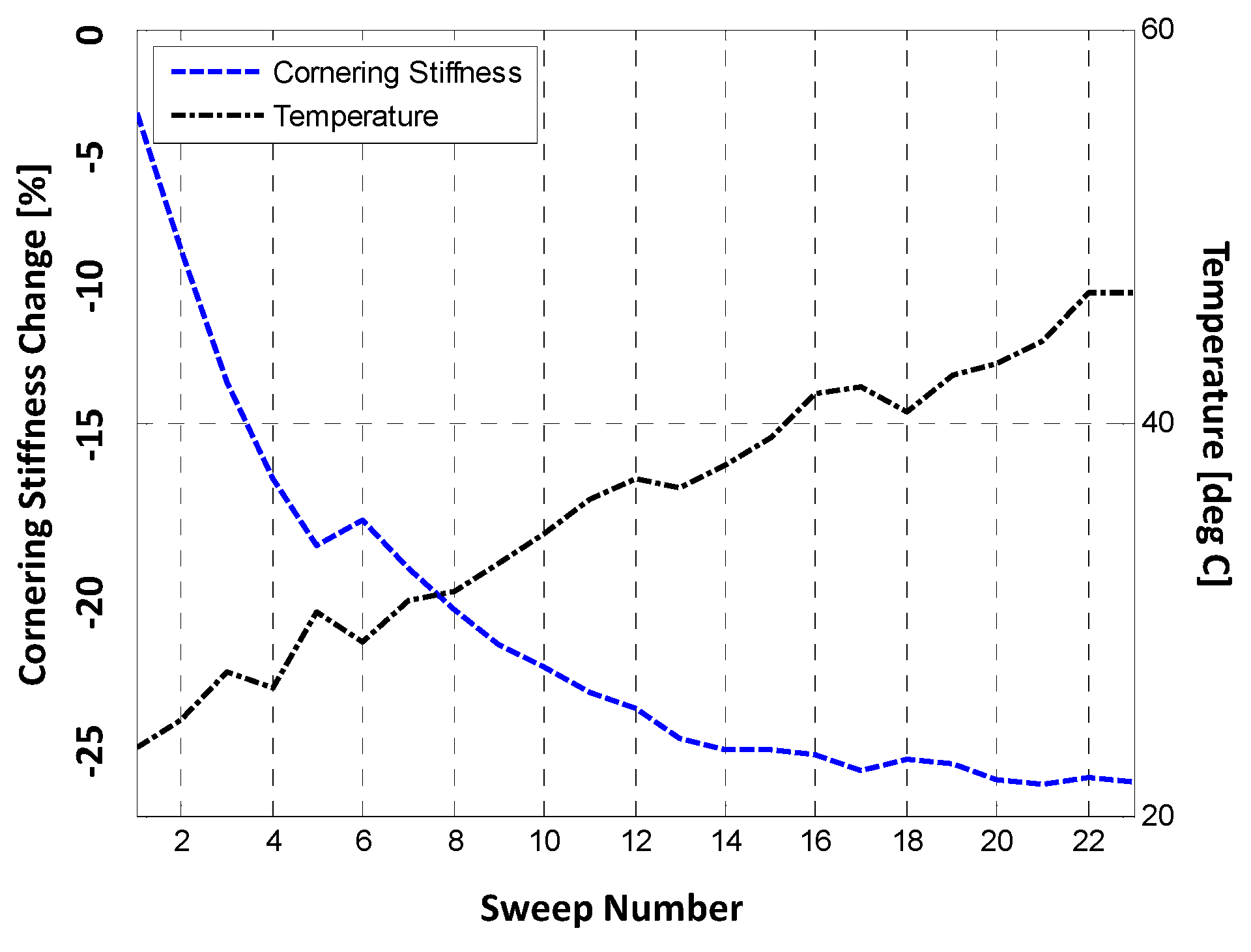
2.4. Influence of Temperature on the Tire Characteristics of Interest
- The storage modulus or tread rigidity, which influences cornering stiffness. This changes due to the bulk temperature of the tire.
- The coefficient of friction decides the peak lateral grip of the tire. This parameter is only influenced by the surface temperature of the tire at the road interface.
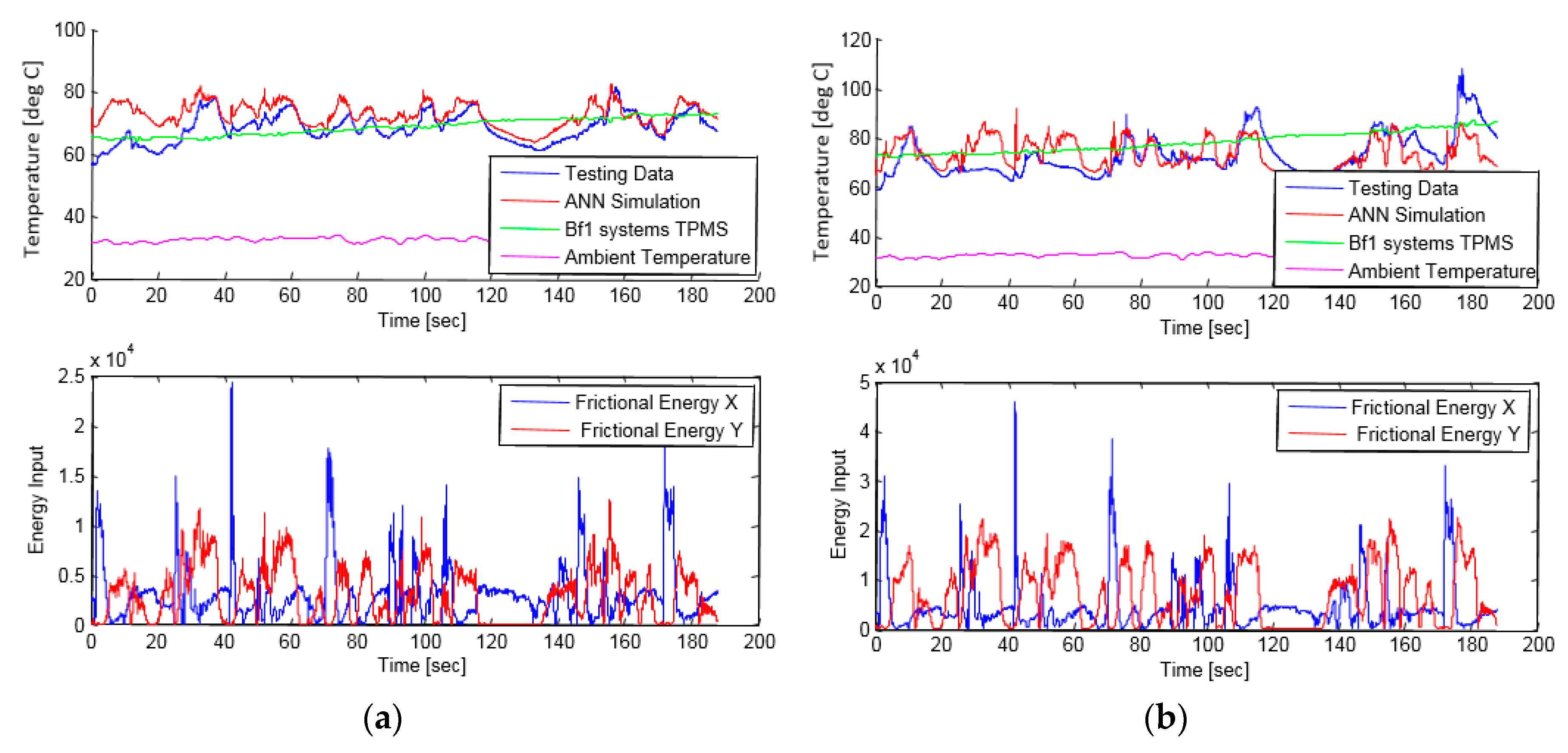
3. Magic Formula (MF) Cornering Stiffness Adaptation
- Inner liner temperature (available from tire attached sensor systems)
- Ambient temperature (from the vehicle controller area network (CAN))
- Frictional energy (estimated using the vehicle CAN signals)
- Forward velocity and vehicle yaw-rate (from the vehicle CAN)
- Temperature at previous time-step (internal model calculation)
4. Vehicle Sideslip Angle Estimation Scheme
- Axle lateral force
- Axle cornering stiffness
- Yaw rate and vehicle speed/velocity
- Both UKF and EKF have been found to be effective at identifying simple or complex vehicle models [35]. Although they use different methods for parameter error covariance estimation, both techniques have identical convergence characteristics and yield near-identical models.
- However, unlike an EKF-based observer, an UKF-based observer avoids the need to calculate Jacobians and is computationally less expensive and easier to implement.
- : fit parameters,
- current operating values of load, pressure, temperature and tread depth,
- Nominal values of load, pressure, temperature and tread depth,
- : Magic Formula parameters at nominal conditions.
Future Research Steps
5. Conclusions
Funding
Conflicts of Interest
References
- Piyabongkarn, D.; Rajesh, R.; John, A.G.; Jae, Y.L. Development and experimental evaluation of a slip angle estimator for vehicle stability control. IEEE Trans. Control Syst. Technol. 2009, 17, 78–88. [Google Scholar] [CrossRef]
- Selmanaj, D.; Matteo, C.; Giulio, P.; Sergio, M.S. Vehicle sideslip estimation: A kinematic based approach. Control Eng. Pract. 2017, 67, 1–12. [Google Scholar] [CrossRef]
- Oh, J.; Choi, S.B. Dynamic sensor zeroing algorithm of 6D IMU mounted on ground vehicles. Int. J. Automot. Technol. 2013, 14, 221–231. [Google Scholar] [CrossRef]
- Sierra, C.; Tseng, E.; Jain, A.; Peng, H. Cornering stiffness estimation based on vehicle lateral dynamics. Veh. Syst. Dyn. 2006, 44, 24–38. [Google Scholar] [CrossRef]
- Lundquist, C.; Schön, T.B. Recursive identification of cornering stiffness parameters for an enhanced single track model. IFAC Proc. Volumes 2009, 42, 1726–1731. [Google Scholar] [CrossRef]
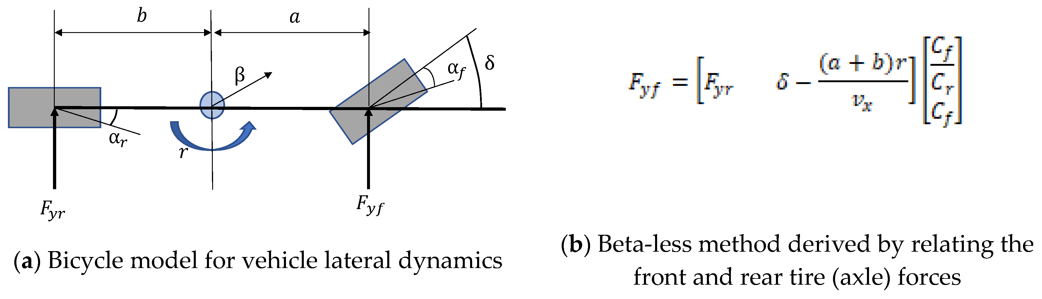
- Viehweider, A.; Nam, K.; Fujimoto, H.; Hori, Y. Evaluation of a betaless instantaneous cornering stiffness estimation scheme for electric vehicles. In Proceedings of the 2012 9th France-Japan & 7th Europe-Asia Congress on Mechatronics (MECATRONICS) / 13th Int’l Workshop on Research and Education in Mechatronics (REM), Paris, France, 21–23 November 2012. [Google Scholar]
- Jain, S. Estimation of vehicle handling states. Master’s Thesis, Delft University of Technology, Delft, the Nederland, 2014. [Google Scholar]
- Wan, E.A.; Rudolph, V.D.M. The unscented Kalman filter for nonlinear estimation. In Proceedings of the IEEE 2000 Adaptive Systems for Signal Processing, Communications, and Control Symposium (Cat. No.00EX373), Lake Louise, AB, Canada, 4 October 2000. [Google Scholar]
- Bechtloff, J.; Ackermann, C.; Isermann, R. Adaptive state observers for driving dynamics–online estimation of tire parameters under real conditions. In 6th International Munich Chassis Symposium 2015; Springer Vieweg: Wiesbaden, Germany, 2015. [Google Scholar]
- Bechtoff, J.; Koenig, L.; Isermann, R. Cornering Stiffness and Sideslip Angle Estimation for Integrated Vehicle Dynamics Control. IFAC-PapersOnLine 2016, 49, 297–304. [Google Scholar] [CrossRef]
- Goodyear Dunlop Reveals Intelligent Tire Concept at Geneva Motor Show. Available online: https://www.goodyear.eu/corporate_emea/news-press/articles/goodyear-dunlop-reveals-intelligent-tire-concept-at-geneva-motor-show-_156593 (accessed on 8 February 2019).
- Bridgestone Announces Development of New Technology for Estimating Tire Wear Based on the Concept of CAIS. Available online: https://www.automotiveworld.com/news-releases/bridgestone-announces-development-new-technology-estimating-tire-wear-based-concept-cais/ (accessed on 8 February 2019).
- Pirelli Introduces ’Smart’ Tires in Geneva. Available online: https://www.moderntiredealer.com/news/721340/pirelli-introduces-smart-tires-in-geneva-and-will-debut-them-in-the-u-s (accessed on 7 February 2019).
- Continental iTires: Intelligent Tires Shipped from the Factory. Available online: https://www.continental-tires.com/transport/media-services/newsroom/20160921-itire (accessed on 7 February 2019).
- Pacejka, H. Tire and Vehicle Dynamics; Elsevier: Oxford, UK, 2005. [Google Scholar]
- Schillinger, J.; Rainer, V.L.; Adrian, C.; Joerg, L. Sensor transponder and procedure for measuring tire contact lengths and wheel load. U.S. Patent 7,536,903, 26 May 2009. [Google Scholar]
- Wagner, M.; Hendrik, T. Method for monitoring the load of vehicle tires. U.S. Patent 8,742,911, 3 June 2014. [Google Scholar]
- Mancosu, F.; Massimo, B.; Daniele, A. Method and system for determining a cornering angle of a tyre during the running of a vehicle. U.S. Patent 8,024,087, 20 September 2011. [Google Scholar]
- Hanatsuka, Y.; Hiroshi, M. Road surface condition estimating method, road surface condition estimating tire, road surface condition estimating apparatus, and vehicle control apparatus. U.S. Patent 9,046,457, 2 June 2015. [Google Scholar]
- Tebano, R.; Glorgio, A. Method and system for determining the potential friction between a tyre for vehicles and a rolling surface. U.S. Patent 8,626,454, 7 January 2014. [Google Scholar]
- Singh, K.B.; Mustafa, A.A.; Saied, T. An intelligent tire based tire-road friction estimation technique and adaptive wheel slip controller for antilock brake system. J. Dyn. Syst. Meas. Contrl. 2013, 135, 031002. [Google Scholar] [CrossRef]
- Teerhuis, A.; Schmeitz, A.J.C.; Molengraft-Luijten, L. Tire state estimation based on measured accelerations at the tire inner liner using an extended Kalman filter design. In Proceedings of the 4th International Tyre Colloquium, Tyre Models for Vehicle Dynamics Analysis, University of Surrey, Guildford, the United Kingdom, 20–21 April 2015. [Google Scholar]
- Hanatsuka, Y. Method and apparatus for detecting wear of tire. U.S. Patent 8,061,191, 22 November 2011. [Google Scholar]
- Brusarosco, M.; Federico, M. Method and system for wear control of vehicle tyres. U.S. Patent 8,775,017, 8 July 2014. [Google Scholar]
- Lehmann, J.; Bernd, L. Method for determining the depth of tread of a vehicle tire with a tire module arranged on the inner side of the tire. U.S. Patent Application 14/642,114, 9 March 2015. [Google Scholar]
- I.B.A.o.h. Veld, Enhancing the MF-Swift Tyre Model for Inflation Pressure Changes. Available online: https://pure.tue.nl/ws/files/46975582/674114-1.pdf (accessed on 1 November 2007).
- Février, P.; Martin, H.; Fandard, G. Method for simulating the thermomechanical behaviour of a tyre rolling on the ground. U.S. patent US8290756B2, 16 October 2012. [Google Scholar]
- Février, P. Thermal and Mechanical Tire Force & Moment Model presentation. In Proceedings of the 4th IPG Technology Conference, Ettlingen, Baden-Württemberg, Germany, 23–24 September 2008. [Google Scholar]
- Sebastien, C. Tire Thermal Analysis And Modeling. Master’s Thesis, Chalmers University of Technology, Göteborg, Sweden, 2011. [Google Scholar]
- Mizuno, M. Development of tire side force model based on magic formula with the influence of tire surface temperature. R&D Review of Toyota CRDL 2003, 38, 17–22. [Google Scholar]
- Sorniotti, A.; Velardocchia, M. Enhanced Tire Brush Model for Vehicle Dynamics Simulation; SAE Technical Paper; SAE World Congress & Exhibition: Detroit, MI, USA, 2008. [Google Scholar] [CrossRef]
- Pasterkamp, W.R.; Hans, B.P. Application of neural networks in the estimation of tire/road friction using the tire as sensor; SAE Technical Paper; SAE International Congress and Exposition: Detroit, MI, USA, 1997. [Google Scholar]
- Singh, K.B. Development of an intelligent tire based tire-vehicle state estimator for application to global chassis control. Master’s Thesis, Virginia Tech, Blacksburg, VA, USA, 2012. [Google Scholar]
- Singh, K.B. Tire wear state estimation system utilizing cornering stiffness and method. U.S. Patent 13/973,262, 26 February 2015. [Google Scholar]
- Bogdanski, K.; Matthew, C.B. Kalman and particle filtering methods for full vehicle and tyre identification. Veh. Syst. Dyn. 2017, 56, 1–22. [Google Scholar] [CrossRef]
- Doumiati, M.; Victorino, A.; Daniel, L.; Baffet, G.; Charara, A. Observers for vehicle tyre/road forces estimation: Experimental validation. Veh. Syst. Dyn. 2010, 48, 1345–1378. [Google Scholar] [CrossRef]
- Cho, W.; Jangyeol, Y.; Seongjin, Y.; Bongyeong, K.; Kyongsu, Y. Estimation of tire forces for application to vehicle stability control. IEEE Trans. Veh. Technol. 2010, 59, 638–649. [Google Scholar]
- Niessen, B.C.; Jansen, S.T.H.; Besselink, I.J.M.; Schmeitz, A.J.C.; Nijmeijer, H. An enhanced generic single track vehicle model and its parameter identification for 15 different passenger cars. In Proceedings of the 11th International Symposium on Advanced Vehicle Control (AVEC 2012), Seoul, Korea, 9 September–9 December 2012. [Google Scholar]
- Niskanen, A. Sensing the tyre-road contact by intelligent tyre. Ph.D. Thesis, Aalto University, Espoo, Finland, 2017. [Google Scholar]
- Singh, K.B.; Saied, T. Estimation of tire–road friction coefficient and its application in chassis control systems. Syst. Scim Cont. Eng. 2015, 3, 39–61. [Google Scholar]
- Hanatsuka, Y.; Yasumichi, W.; Hiroshi, M. Method for estimating road surface condition. U.S. Patent 9,170,102, 27 October 2015. [Google Scholar]
- Matilainen, M.; Ari, T. Tyre contact length on dry and wet road surfaces measured by three-axial accelerometer. Mech. Syst. Sig. Process. 2015, 52, 548–558. [Google Scholar] [CrossRef]


| Approach | Underlying Principle | Reference |
|---|---|---|
| Model Based Observer | The sideslip angle model is typically based on the bicycle model. The model can further include feedback of error signals (the differences between the measured signals and the ones predicted by the model), thus forming a closed loop observer | [1] |
| Kinematic Based Observer | Rely on kinematic equations correlating the vehicle longitudinal and lateral velocities with longitudinal and lateral accelerations and the yaw-rate. These methods do not depend on vehicle or tire–road friction parameters | [2] |
| Influencing Factor | Effect on the Tire Cornering Stiffness | Reasoning |
|---|---|---|
| Inflation Pressure | Moderate | Caused by a variation in the carcass stiffness and tread stiffness |
| Tire Wear | High | Caused by a variation in the tread stiffness |
| Tire Temperature | High | Caused by a variation in the rubber elasticity |
| Tire Aging | High | Caused by stiffening on tread rubber |
| Measured Signal | Underlying Physics | Reference |
|---|---|---|
| Tangential acceleration | Monitors change in the tire vibrational characteristics between the frequency range 1000–3000 Hz | U.S. Patent 8061191 [23] |
| Radial acceleration | Monitor radial acceleration in the pre-footprint region between frequency range 1000–1700 Hz | U.S. Patent 8775017 [24] |
| Radial acceleration | Monitors change in the tire internal radius | U.S. Patent 9764603 [25] |
| Tire Surface Temperature | Tire Bulk Temperature | Inflation Pressure | Normal Load | Speed | Tread Depth | |
|---|---|---|---|---|---|---|
| Cornering Stiffness | x (∼constant) | x (∼constant) | ✓ | ✓ | x (constant) | ✓ |
| Tire Surface Temperature | Tire Bulk Temperature | Inflation Pressure | Normal Load | Rolling Speed | Tread Depth | |
|---|---|---|---|---|---|---|
| Cornering Stiffness (CS) | High Dependency | High Dependency | High Dependency | High Dependency | Negligible Dependency | High Dependency |
| Tire Type | Factors Influencing Tire Characteristics | |||
|---|---|---|---|---|
| Pressure | Tread Depth | Temperature | ||
| Summer Tire (High Performance) | Cornering Stiffness | 10% increase with a 20% change in inflation pressure from nominal conditions | 30% increase with a 60% decrease in tread depth | 20–25% drop from cold to hot tire conditions (* strongly influenced by the tire bulk temperature) |
| Parameter | Value |
|---|---|
| α | 1 × 10⁻³ |
| β | 2 |
| Κ | 0 |
| State Estimated | Underlying Physics | Reference |
|---|---|---|
| Tire road friction | Friction potential estimated through frequency domain analysis of the accelerometer signals | [39,40,41] |
| Tire aquaplaning propensity | Remaining tire road contact length is determined based on the tangential acceleration signal | [39,42] |
| Water depth | To detect the presence of water in the tire–road contact, the lateral acceleration signal is utilized. Since normal excitation from the road surface is lowest in the lateral direction, all external excitation produces rather noticeable difference. | [39] |
© 2019 by the author. Licensee MDPI, Basel, Switzerland. This article is an open access article distributed under the terms and conditions of the Creative Commons Attribution (CC BY) license (http://creativecommons.org/licenses/by/4.0/).
Share and Cite
Singh, K.B. Vehicle Sideslip Angle Estimation Based on Tire Model Adaptation. Electronics 2019, 8, 199. https://doi.org/10.3390/electronics8020199
Singh KB. Vehicle Sideslip Angle Estimation Based on Tire Model Adaptation. Electronics. 2019; 8(2):199. https://doi.org/10.3390/electronics8020199
Chicago/Turabian StyleSingh, Kanwar Bharat. 2019. "Vehicle Sideslip Angle Estimation Based on Tire Model Adaptation" Electronics 8, no. 2: 199. https://doi.org/10.3390/electronics8020199
APA StyleSingh, K. B. (2019). Vehicle Sideslip Angle Estimation Based on Tire Model Adaptation. Electronics, 8(2), 199. https://doi.org/10.3390/electronics8020199