1. Introduction
Nowadays, the industry is changing its organizational structure. This change is known as Industry 4.0, which is intended to improve the economy sector. Companies will become more intelligent by using diverse techniques [
1]. To make this possible, new programmable logic controller (PLC) devices will be introduced, which will transfer huge calculation and information capabilities, and will also be used to introduce more robots in production lines etc. Apart from introducing new devices, there will also be increased connectivity into the same information system. As a result, production can be adapted to demand and become more efficient [
2]. In the end, the aim is to have a greater production capability, better quality, and optimization in production resources.
Robotics is changing the production concept and adapting to this new era. Today, robots and humans work in the same areas. Djuric et al. [
3] commented that these robots are known as Cobots. Thanks to power and force limitations, the employees can stay together in the same working area. According to Cherubini et al. [
4], when they are cooperating, ergonomic concerns can be reduced, due to the physical job and cognitive loading. It also provides improvements on safety, quality, and productivity.
In order to obtain greater flexibility and efficiency, not only will the robots change, but the autonomous guided vehicle (AGV) also introduces new updates. Nowadays, these AGVs only move using magnetic fields, so they do not have any intelligence, which makes it too difficult to change logistics areas [
5]. However, to introduce a free navigation intelligence, mapping, localization, path planning, and path following aspects have to be implemented.
Mapping and localization are solved using simultaneous localization and mapping (SLAM) [
6,
7]. Considering the mobile robot has no idea about where it is and where it is going to be, with SLAM it is possible to learn the environment characteristics in order to locate the vehicle. In the case that it was necessary to move it, another algorithm would be required. Here is where path planning and path following take part. Elsheikh et al. [
8] confirmed, the differences between these, lie in how much the robot can do.
In path planning, the start and end points are given and then the vehicle must plan the best path. The robot navigation problem can be described as the process of determining a suitable and safe path, avoiding obstacles and collisions [
9], therefore, the AGV navigates without any path following restrictions and moves wherever it wants to arrive at its goal position. There are different alternatives which can be implemented, such as swarm optimization (SO), which is based on particle swarm optimization as Ever [
10] analysed, Hu et al. [
11] studied dynamic path planning, and dynamic movements primitives is explained by Mei et al. [
12].
Apart from these, there are other well-known path planning algorithms, such as the dynamic window approach developed by Fox et al. [
13], vector field histogram related by Borenstein et al. [
14], TangentBug and PointsBug, as compared by Buniyamin et al. [
15], and the rapidly exploring random tree, as Adiyatov et al. [
16] explained. Most of these well-known algorithms are used in actual applications.
Otherwise, in path following problems, the user gives the robot the path and it should only follow it. According to Wang [
17], these controllers are designed to obtain the minimal lateral distance, as well as the heading between the vehicle and the command path to control the vehicle speed and steering to follow a specified path. Algorithms like pure pursuit [
18] mentioned, moving to a point [
19], and proportional navigation [
20].
Sebi et al. [
21] advised that apart from using SLAM, path following, and path planning, another algorithm is required. Without any obstacle avoidance intelligence, the AGV makes a safety stop to prevent collision with an object. This is the reason for the proposal of different obstacle avoidance algorithms [
22,
23,
24]. In most cases the obstacles are detected using cameras, LIDAR, or ultrasonic sensors as Amin et al. [
25] and Martinez et al. [
26] explained. In the end, all of these sensors are trying to avoid making contact with the obstacle. However, there are some cases, that when the obstacle is detected as making a collision, the force is analyzed with piezoelectric sensors like Wooten et al. [
27] studied.
The main goal of the present study is to improve a simple path following algorithm introducing an obstacle avoidance technique. This technique is implemented using simple equations, in order to avoid large calculations in the controller. After developing the algorithm, it will be tested with a traditional motion planning algorithm to analyze the differences between both.
2. Problem Formulation
The aim is to take a commercial AGV from industrial application and use its technology to introduce an obstacle avoidance algorithm. This commercial AGV uses a LIDAR to take information from the surroundings, a programable logic controller (PLC) to control AGV periphery (motors, displays, lights, etc.) and an industrial personal computer (IPC) for the SLAM and path following algorithm. It is remarkable that the only programable hardware is the PLC, and it does not have enough capability to process huge calculations like optimization.
All hardware is connected via Ethernet to synchronize the information. The IPC sends speed and steering commands to the PLC, the PLC sends wheel-odometry information to the IPC, and LIDAR sends information to both the PLC and IPC.
In the Industry, it is better to use known trajectories, which is why these vehicles use only path following algorithms. In general, these algorithms are very simple and cannot avoid an obstacle. Hence, it was decided to implement an obstacle avoidance term into the path following.
Furthermore, the AGV has to arrive at a conveyor transport and synchronize its speeds with the moving target. The collaborative robot that was assembled in the AGV then takes an object from conveyor transport and moves it to another point of the factory. The objective is not to stop the conveyor transport to take that product, in order to reduce production time.
The idea of this paper is to take moving to a point mathematical equations and adapt them to implement avoidance technique. Corke [
19] studied a moving to a point path following algorithm, in which the problem of moving towards a goal point (
) in the plane was analyzed. For this solution, the velocity of the robot considered in Equation (1) is controlled proportionally to the distance from the goal, as analysed in Equation (2).
To steer towards the goal, which is represented in Equation (3), it is considered that
is the proportional controller, and the vehicle-relative angle is analyzed in Equation (4).
Therefore, in the current study, a new obstacle avoidance strategy is proposed to be implemented in the moving to a point technique. It is based on measurement between the vehicle and the obstacle.
Table 1 summarizes all terms and parameters used in this work.
3. Implementation of Obstacle Avoidance
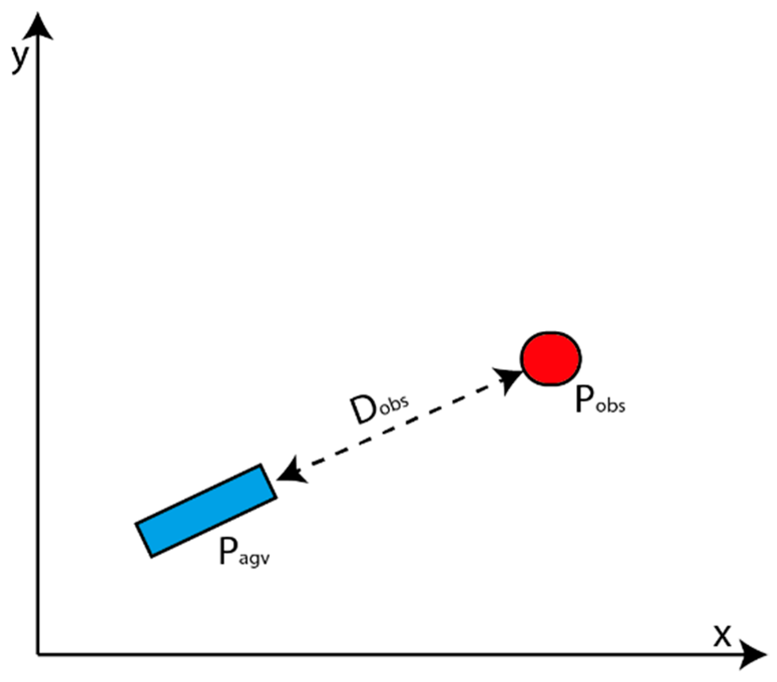
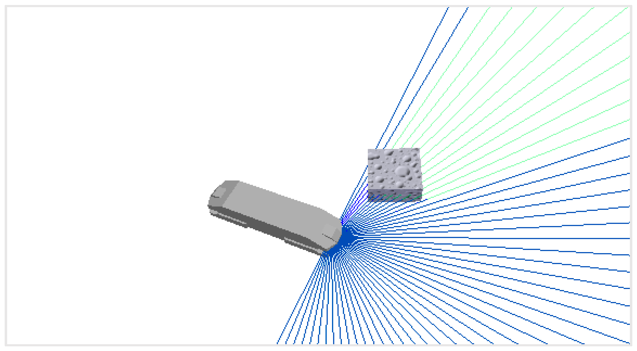
A new formulation is presented in this section, so the vehicle can autonomously correct the path avoiding the obstacle. Considering the measurement of the LIDAR, it is possible to obtain the distance between the AGV and the obstacle. According to Peng et al. [
22], that distance is expressed in Equation (5).
represent the relative coordinates of the distance between the AGV and the nearest obstacle defined by
in
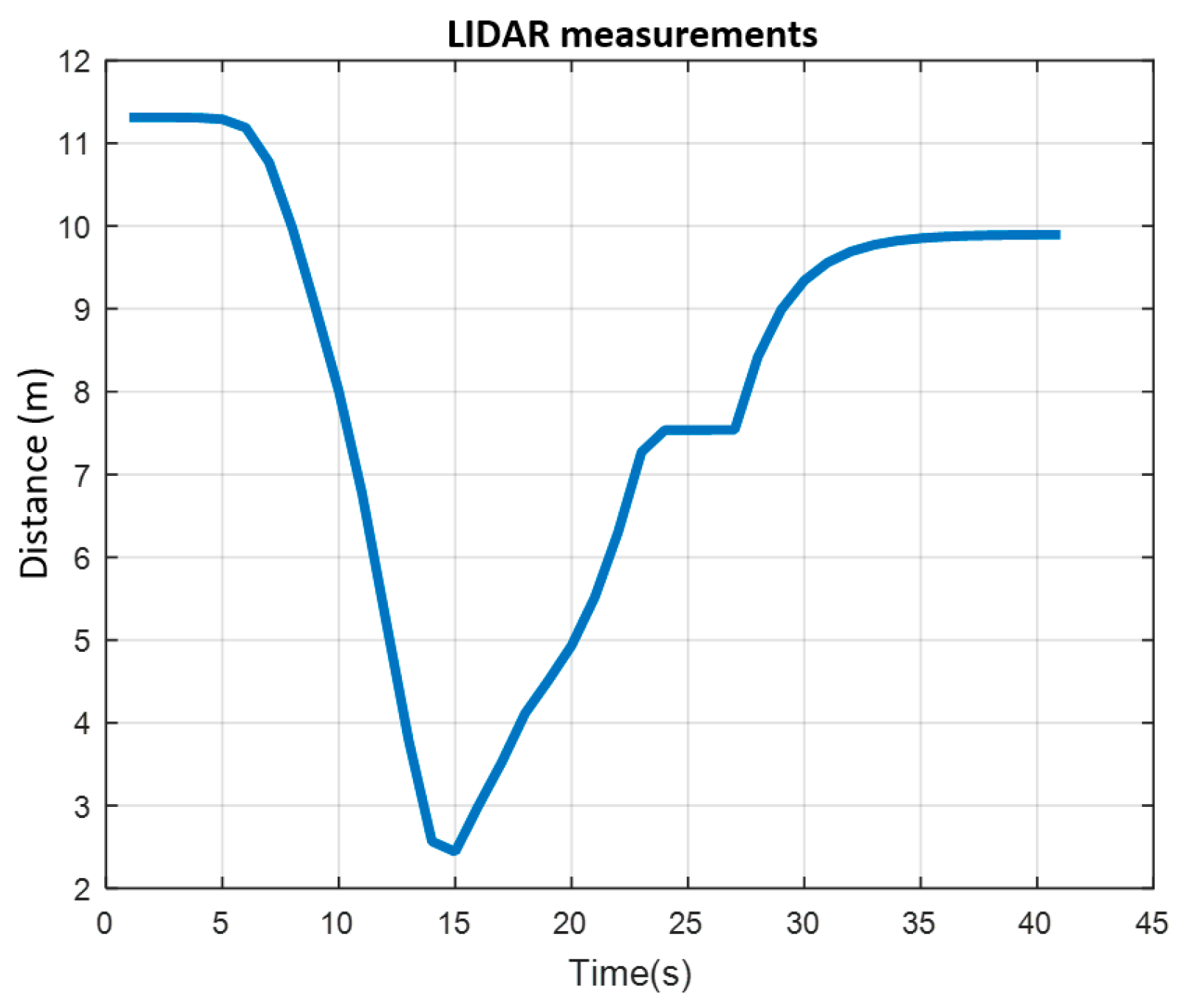
Figure 1. The output of the Equation (5) can be represented in a graph.
Figure 2 shows how the LIDAR measurement changes when some obstacle appears in the AGV’s way.
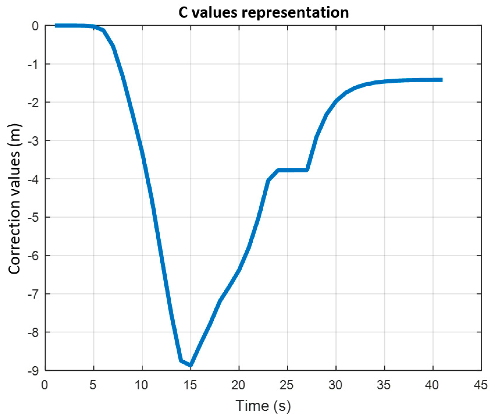
To use that measurement information as a correction for the steering command, the graph must start at 0 value. By subtracting the LIDAR maximum measurement range to
, the answer will change. This way, when the AGV is approaching the obstacle, the value becomes more negative. This expression is analysed in equation (8) and the solution is represented in
Figure 3.
In Equation (9), a safety distance term is introduced to prevent premature correction. This safety distance maintains the AGV direction until the object is between the AGV and that distance. In case of the object being far away, the obstacle avoidance stays in standby mode. In other words, it does not interfere with the moving to a point algorithm.
is a constant which adapts the intensity of the avoid function and
is the safety implementation with a
parameter, which changes the safety distance. This avoid function adapts the AGV direction to avoid the obstacle. Therefore, this term must interact with the
value. Instead of implementing directly the avoidance correction, it has been considered to introduce some logic between the
value and avoid value, using a sigmoid function as shown in Equation (10).
Regrouping all the equations, the Moving to a Point algorithm with obstacle avoidance can be summarized with Equation (11).
where
are constants, which modify the interaction with the Com function.
is a proportional constant, which changes the measurement value to steering value. Until this point, the AGV can avoid an obstacle and it always turns to the right. In some cases, however, it is better to turn to the left so as not to lose too much time avoiding the obstacle. It can be done by analyzing the sign of the angles as represented in Equation (12).
The vehicle velocity can be modified considering the same logic. When the obstacle is close, the AGV must reduce its speed. Taking Equation (9) as reference, Equation (13) can be made, which considers a variation of speed changing
by
.
In addition, this function has to interact with the moving to a point velocity command, which is the reason why Equations (10) and (13) are combined to obtain Equation (14).
where
and
are constants, which modify the interaction with Com function. Finally,
is the proportional value that changes the measurement value to velocity value.
4. AGV Kinematics Equations
In this case, a specific AGV was used, so it is necessary to specify the kinematics of that vehicle. In some cases, it is possible to use defined kinematics like Corke [
19] proposed in his study. This special AGV has two motors in the front axle. The autonomous vehicle uses different speed values in each motor to steer. Both axles are connected mechanically by means of a pulley mechanism to reduce the steering radio.
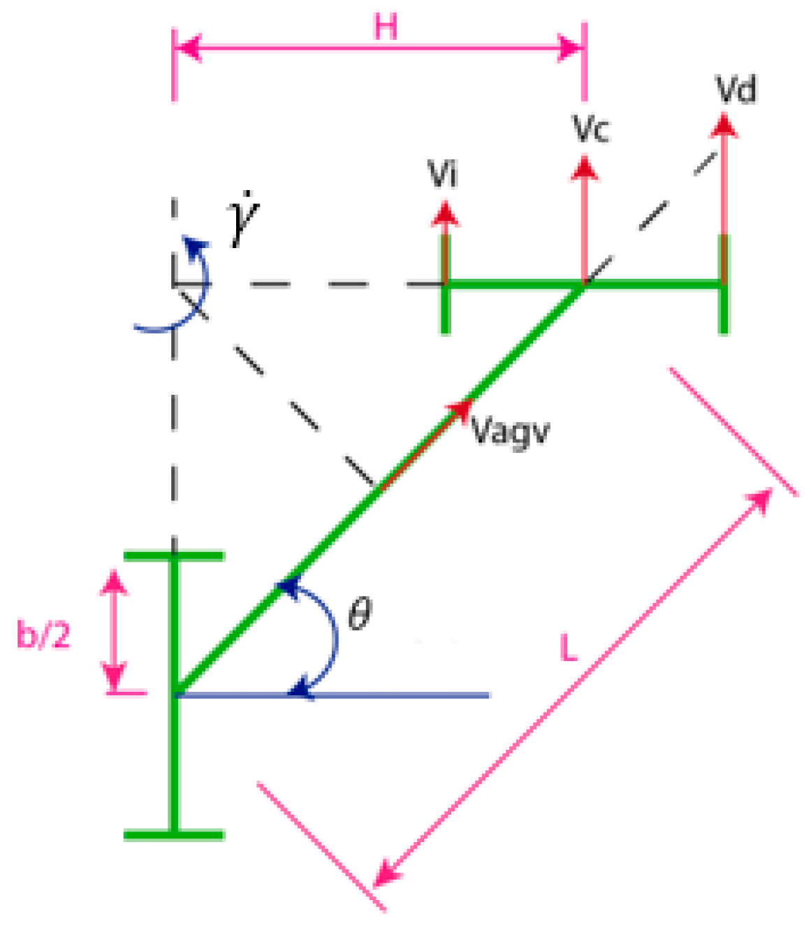
The inputs of the kinematics block are the AGV velocity and direction. The output, however, is the vehicle POSE. The velocity reference () is in the middle of the vehicle. When the AGV goes in a straight line, both motors ( have the same velocity. However, if the AGV takes a curve, the motors will have different velocities.
Hence, taking
Figure 4 as a reference, wheel speed can be represented in Equations (15) and (16):
where
H is the distance between rotation point and
, and b is the size of the wheel axle. Taking into account Equations (15) and (16),
can be defined by motors velocities presented in Equation (17):
The
is split in
and
absolute coordinates.
and
are related each other, since the vehicle is considered as a solid element and the velocity propagates along all the structure, as illustrated in
Figure 5.
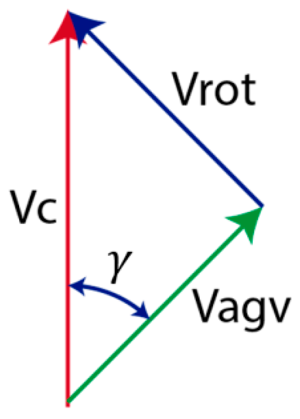
The velocity
represented in
Figure 5 turns the vehicle and generates the rotation in the middle of the AGV. The rotation of the vehicle can be defined with Equations (21) and (22):
Combining (21) and (22), Equation (23) is obtained.
Considering Equations (18–20) and (23), it is possible to define the vehicle dynamics in Equation (24):
where
L is the wheelbase,
is the AGV angle position in absolute coordinates, and
is the value of the direction, which comes from the algorithm.
7. Dynamic Window Approach Comparison
The next step after testing the avoidance algorithm consists of comparing it with a classic motion planning solution. A well-known dynamic window approach (DWA) [
13] algorithm is used. DWA is divided into two parts: The first part is search space, in which the different possible
and
are considered. This section is subdivided into three steps: circular trajectories, where it is calculated a two-dimensional velocity
space, admissible velocities to restrict the admissible velocities ensuring safe trajectories, and dynamic window, which analyses only those velocities that can be reached on a short time interval considering robot acceleration limitations.
The second part is an optimization. The optimization is represented by Equation (25):
Moreover, this second part is also subdivided into three steps: target heading, which is a measure of progress toward the goal, clearance, which is the distance to the closest obstacle, and velocity, which is considered the forward velocity of the robot.
Before starting the simulation of both algorithms, there are some aspects that can be appreciated without any execution. On the one hand, DWA uses an optimization term and normally these equations require a high computational capability. For the AGV that is used in our application, it is impossible to execute and process this optimization over a short period of time. That is the reason for the development of POA. Otherwise, with DWA it is possible to generate a proper trajectory, as it always selects the best path according to the space conditions. Furthermore, POA does not consider the vehicle kinematics, hence it makes a simpler calculation to avoid the obstacle. In order words, POA does not calculate a trajectory, it just modifies the path following command to change the direction and velocity when some obstacle appears in front of the vehicle. As a result, when some object is detected, the speed will be reduced to avoid it safely. DWA, however, always selects a trajectory considering the top speed value and minor acceleration loss.
On the other hand, in both cases adjustable gains are used to optimize the algorithms, making it more flexible to adapt to different surroundings or kinematics conditions. In addition, DWA can select which side turns the vehicle, in order to avoid the obstacle using the trajectory optimization. POA, such as the other algorithm, makes the same action. Otherwise, it uses Equation (12) to determinate which side turns the AGV.
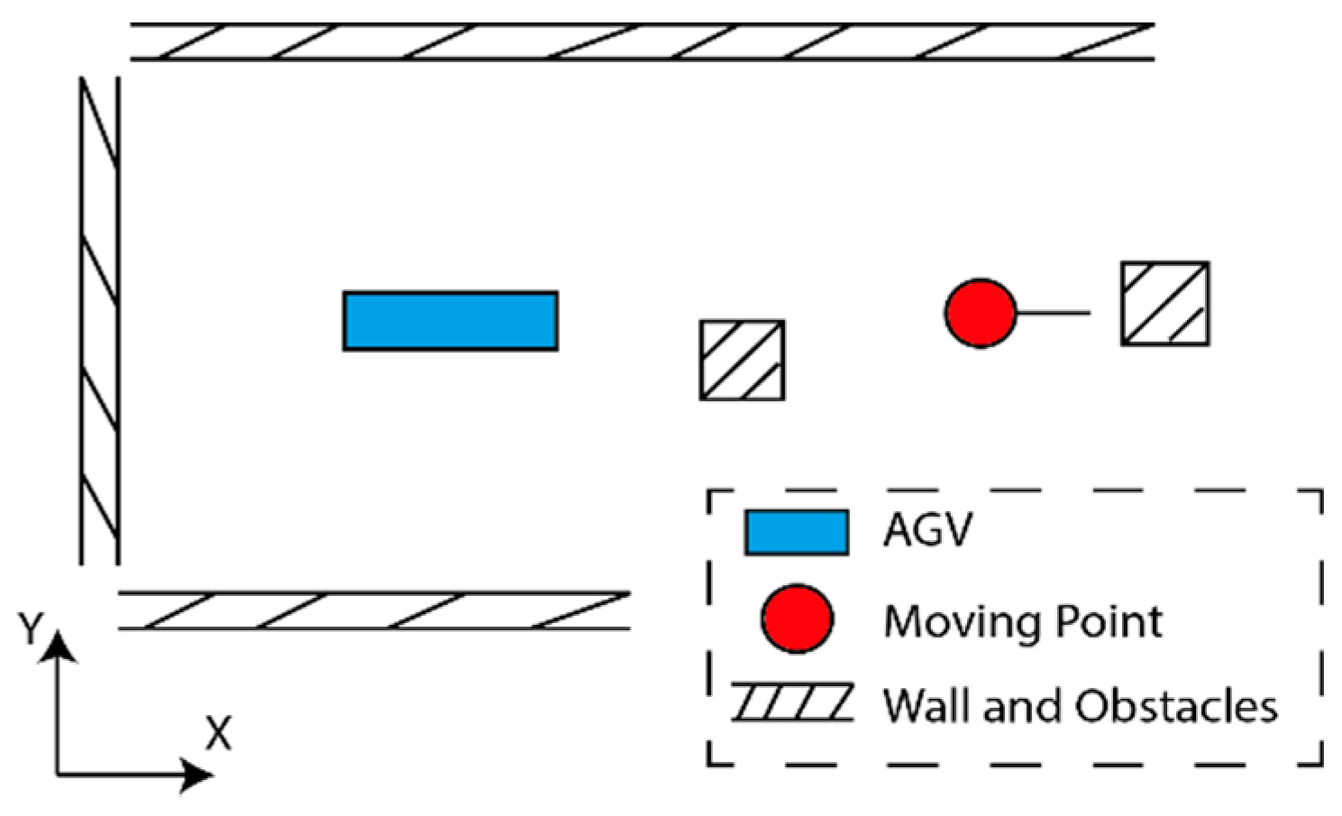
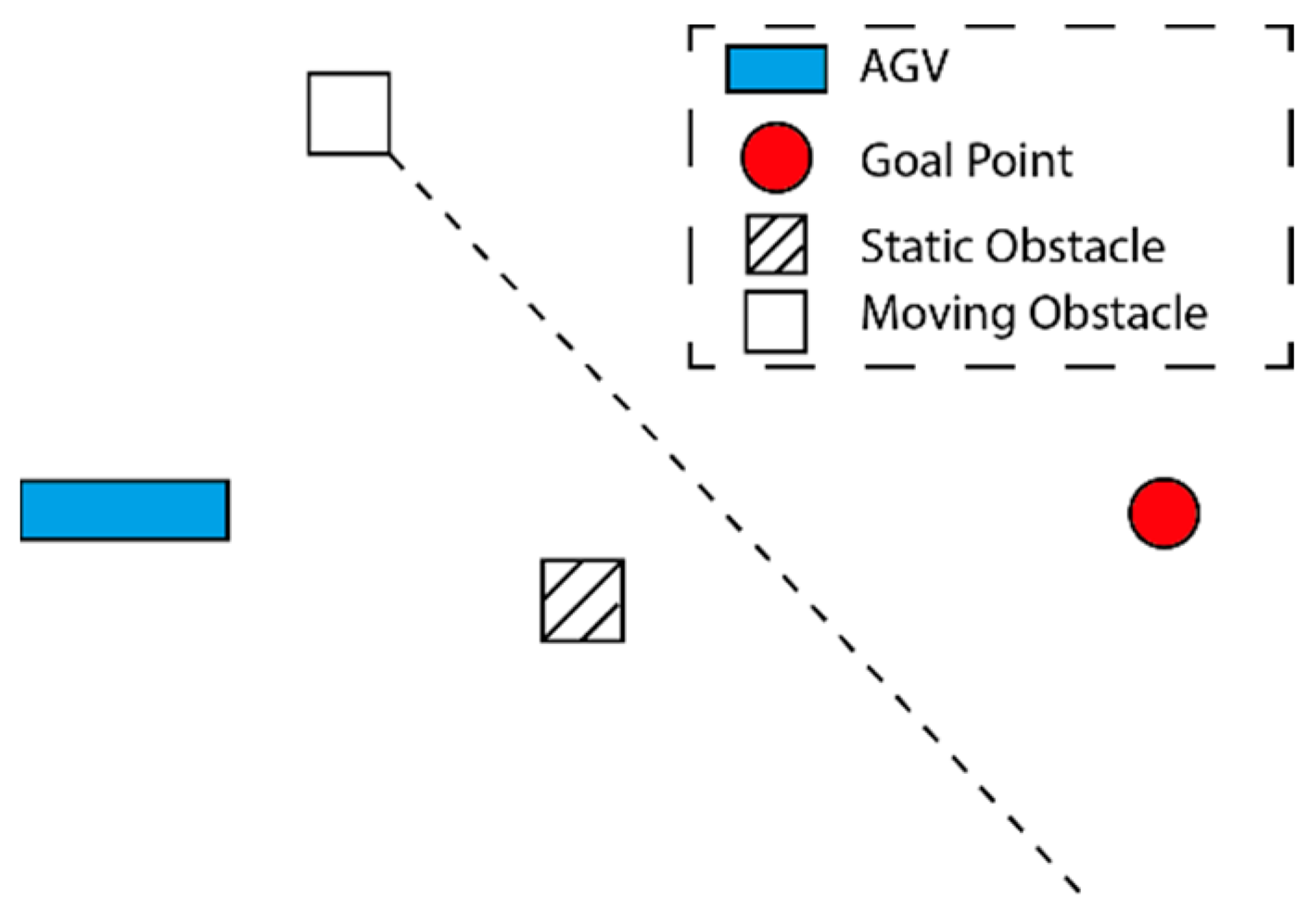
In order to perform an easy comparison between both algorithms, a new simple scenario has been designed (see
Figure 13). There are three elements in the scenario: an object, a moving obstacle, and the static goal position. With the moving obstacle, it is possible to analyze human–robot collaboration. This moving obstacle is considered to be a human and the AGV must avoid the collision.
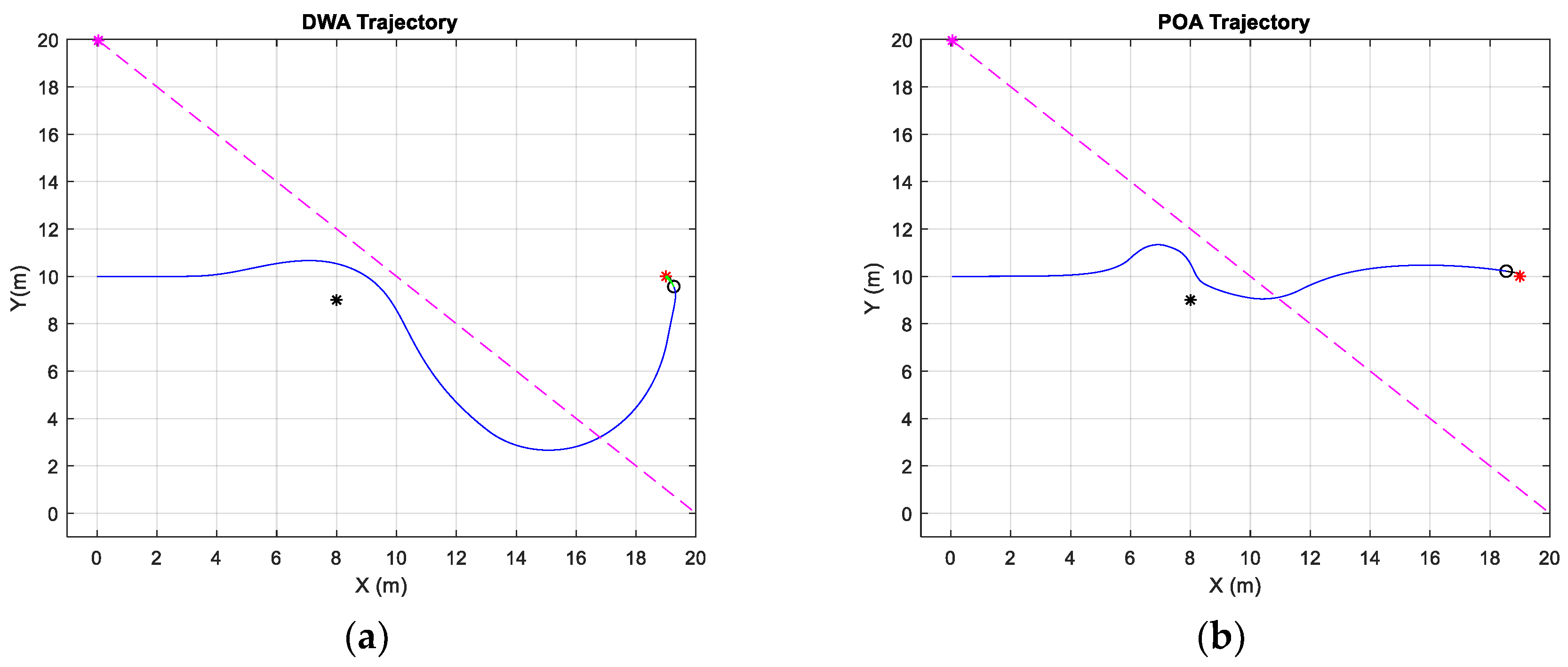
Using
Table 2 variables, the result of both algorithm executions is shown in
Figure 14. Where the black
represents the static obstacle, the red
draws goal point, the pink
represents the moving obstacle, the pink dashed line shows moving obstacle trajectory, green lines represent DWA possible trajectories, and blue lines represent the algorithm trajectory.
For this particular example, the DWA algorithm had more problems to avoid the moving obstacle than POA. DWA, with
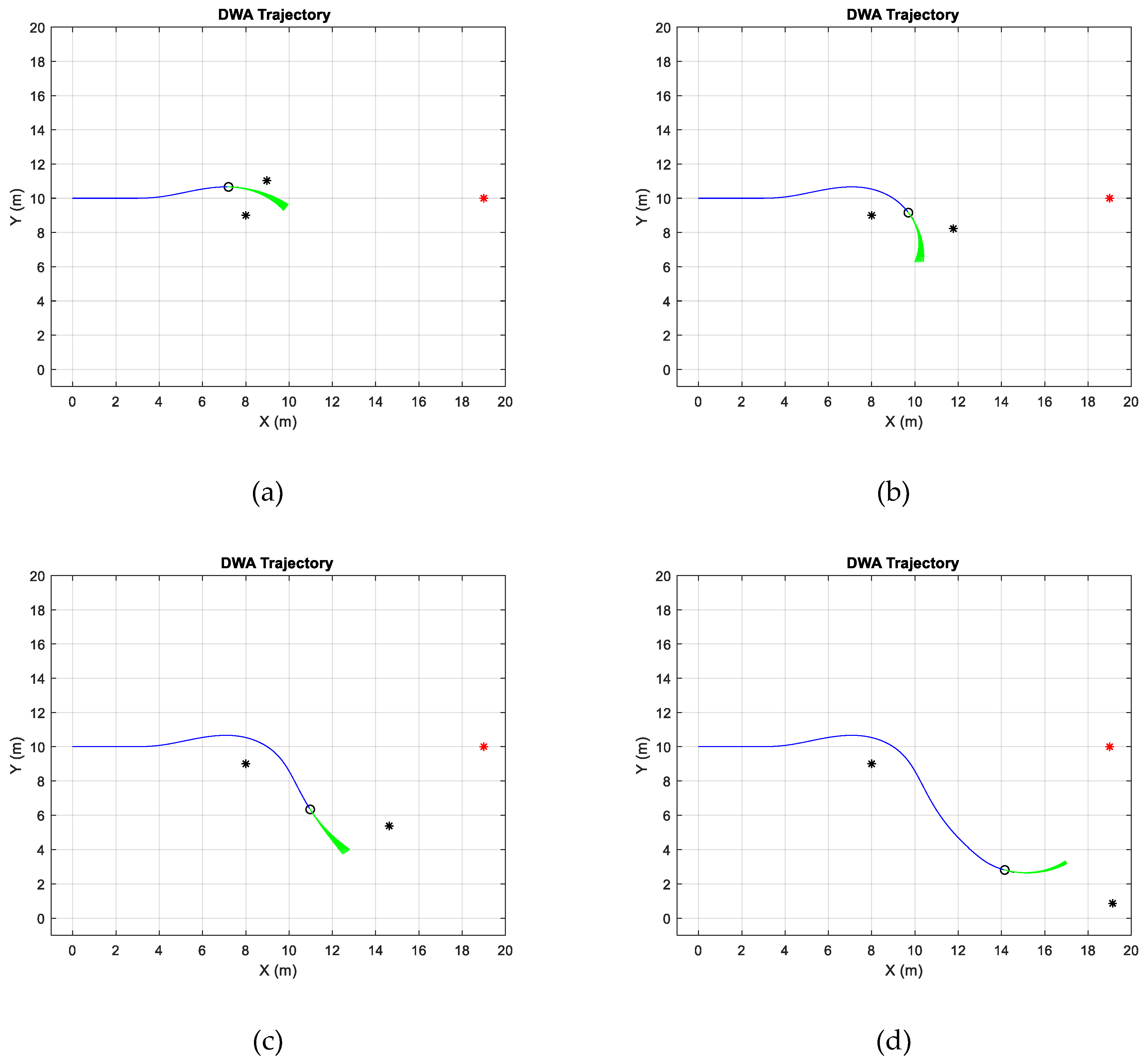
Table 3 optimization constant values, cannot fit an optimal trajectory to avoid the moving obstacle. To have a better idea of how the algorithms act with the mobile object,
Figure 15 represents different time instants of the AGV trajectory. In the end, the algorithm does not avoid the moving obstacle, until the obstacle is a particular distance away from the AGV. Hence, it would be a problem if the vehicle did not have enough
.
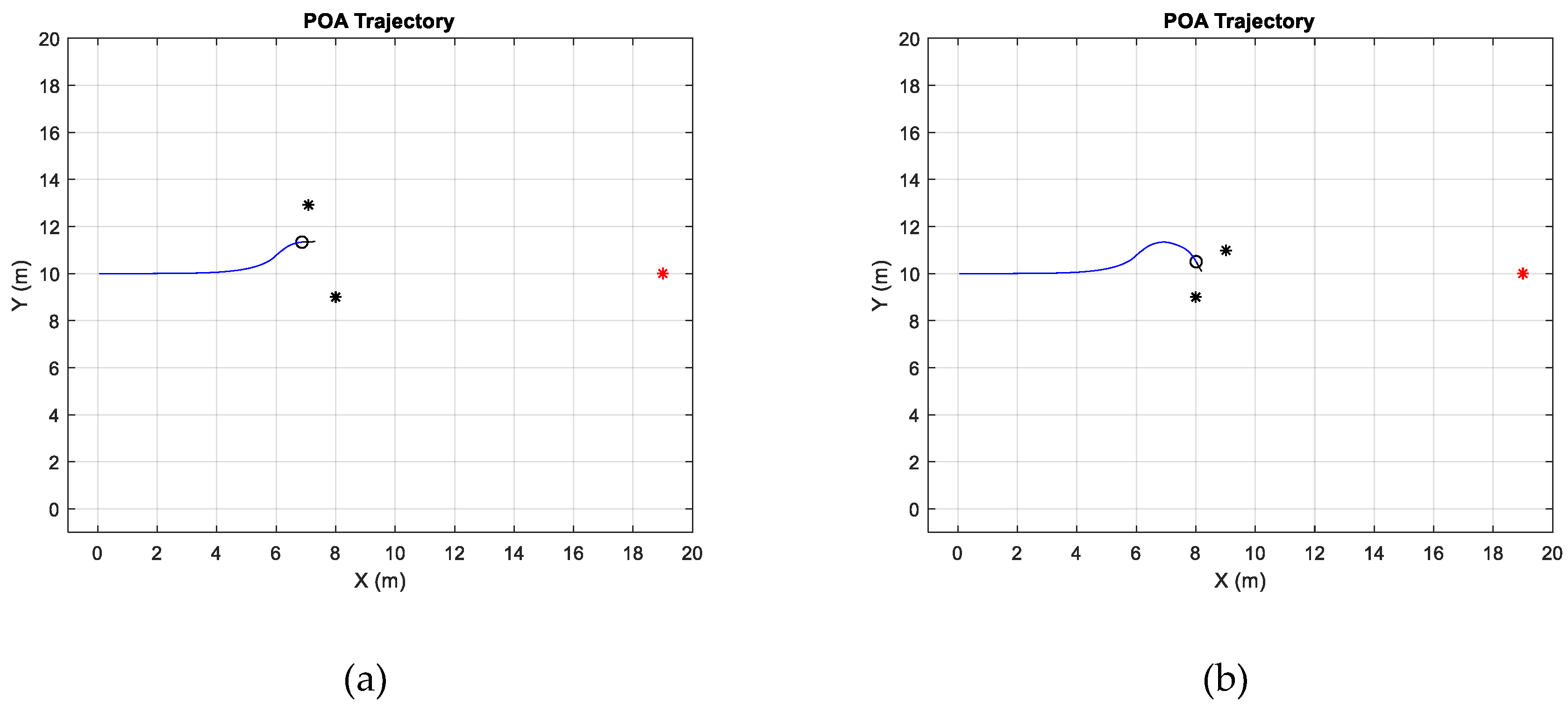
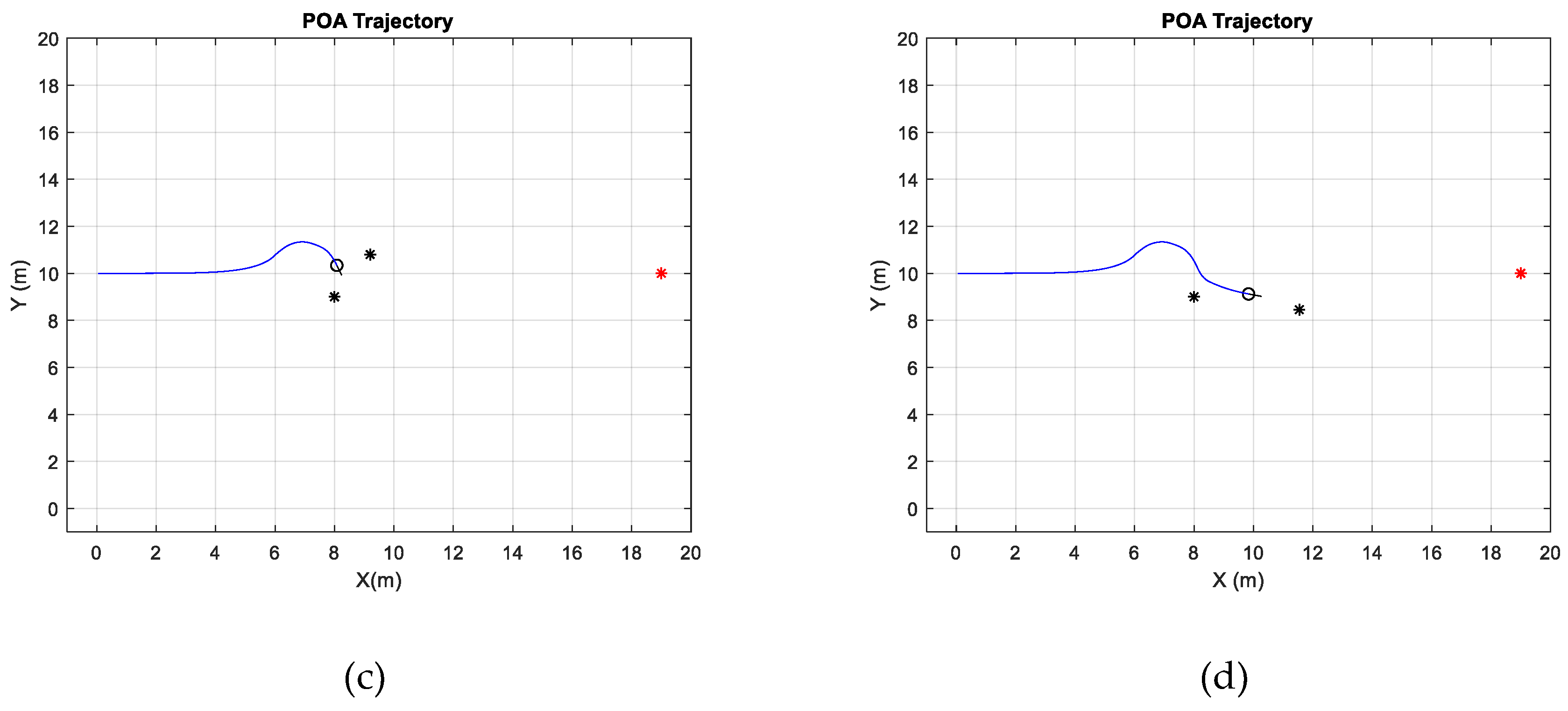
Figure 16 shows the avoidance progress for POA. The POA algorithm tries to avoid the moving obstacle until the sign of Equation (12) changes. When that sign changes, the AGV continues to the goal without any problem.
In order to stop simulating, new different starting points for the AGV are implemented. This makes it possible to analyze and compare what happens with the vehicle on different cases. Apart from this, DWA configurable constants are changed to reduce the speed window size.
is used, in order to reduce the effect that is shown in
Figure 15, in which the AGV needed more
to avoid the obstacle.
In
Table 3 different simulation results are shown, and it is necessary to consider that speed arriving at goal is the speed value at 1 s before arriving to the goal. Additionally, a static object is implemented, which is an x = 8 and y = 9 position, and a moving point, which starts in x = 0 and y = 20 position and ends in x = 40 and y = −20 position with 0.92 m/s constant speed. In addition, the goal is located in an x = 20 y = 20 position. All of these parameters also are used in the
Figure 14 simulation.
Looking at
Table 3, in general, DWA needs more space to avoid the obstacles with this configuration. That is why the value of
is larger than POA. Hence, the odometry in DWA is going to be higher, because both parameters are proportional.
If total time is compared, however, the situation changes. POA uses more time to arrive at the goal position. When AGV is approximating the goal, it will reduce the speed more dramatically, as represented by the speed arriving at goal column. In the end, the difference between both approximation speeds is around 0.46 m/s. Otherwise, POA has the best mean speed and the difference between both mean speeds is about 0.07 m/s, which is negligible.
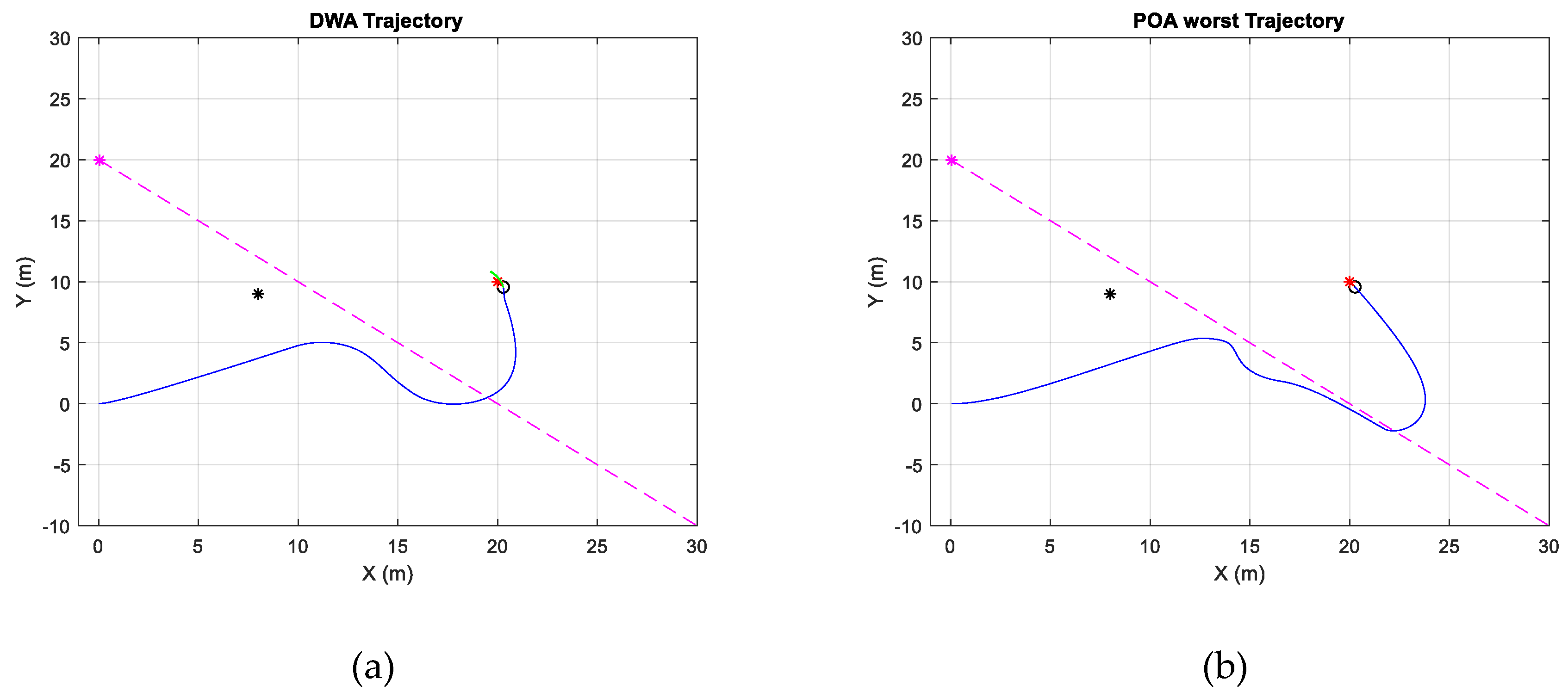
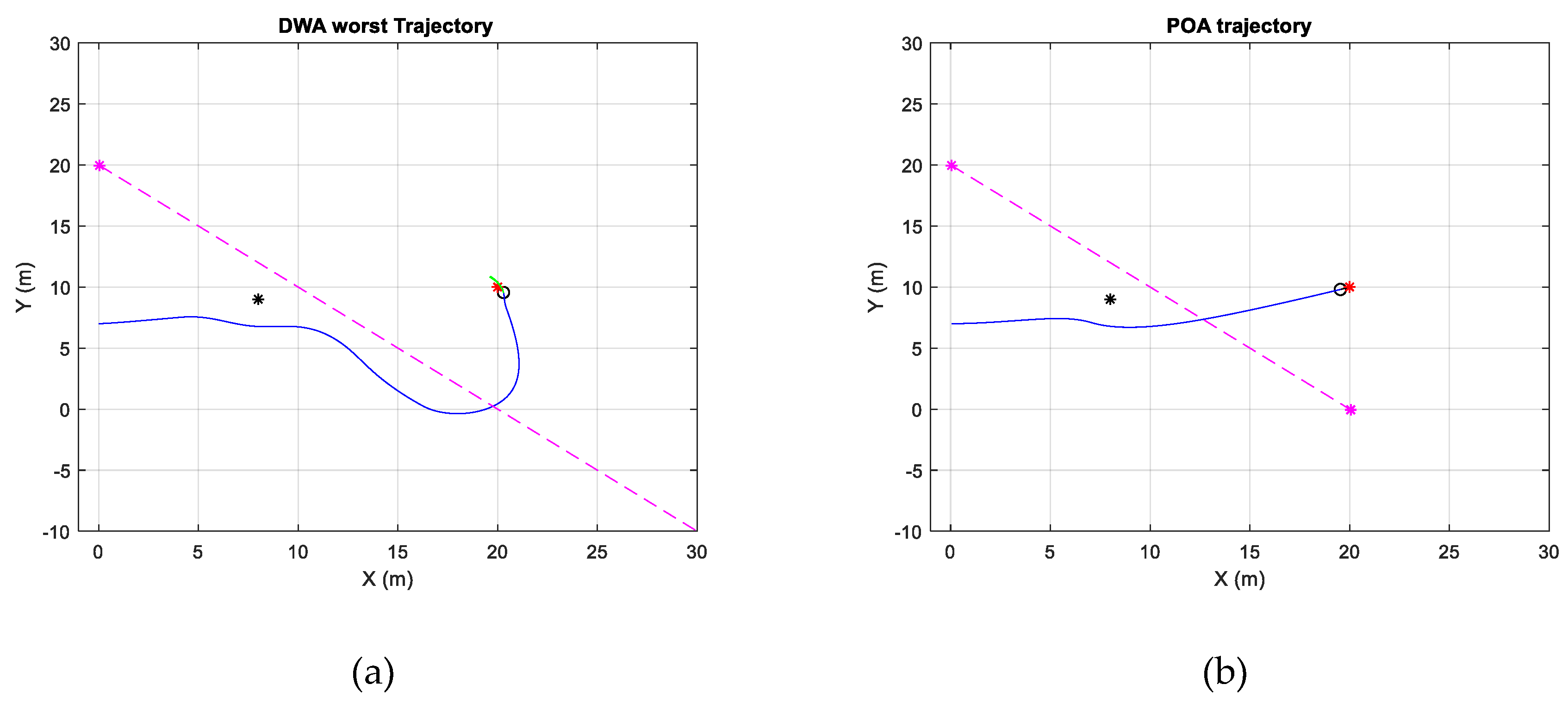
To give a general idea about algorithms failure,
Figure 17, which represents the worst trajectory of POA in comparison with DWA, and
Figure 18, which analyzes the worst trajectory of DWA in comparison with POA, are shown. To consider which is the worst trajectory, the largest odometry was analyzed, due to AGV diverting more from the ideal path, which is a straight line from the starting point to the goal.
In
Figure 17, POA had a greater difficulty deciding where to avoid the moving obstacle. AGV tried to follow it until the obstacle was so far away that the vehicle stopped detecting it. A similar occurrence is observed in
Figure 18. Instead of POA failing to avoid the obstacle, this time DWA failed. The dynamic window did not have enough space to pass the obstacle and it waited until having enough distance to avoid it. In both cases, the algorithms have a bad reaction with the moving obstacle, hence for future work it could be possible to analyze the space and detect moving obstacles. In case that some moving obstacle appears, the AGV stops and wait until the obstacle disappears.
Overall, both algorithms work in the same conditions, though depending on the algorithm configuration the answer of the simulation can change. There are some cases in which the DWA trajectories are worst, and other times the POA’s paths are not good enough. Generally, DWA approximates the goal with a higher speed and, depending on the application, this speed must be controlled to safely arrive. POA, however, gives less space between the AGV and object. In the end, this could be a problem if the AGV moves around humans.
8. Conclusions
The solution proposed in this paper can highly improve a simple path following algorithm behavior. It gives more intelligence to the AGV, a result of the obstacle avoidance parameters. Moreover, it introduces more flexibility to the algorithm, because there are some variables which change the performance. Additionally, POA uses a simple equation to implement on a PLC, which is the only hardware available on the selected AGV. This hardware limitation is an important feature, because not all equipment supports large calculation capabilities, such as DWA, which uses an optimization function to select the best trajectory.
The optimization function gives the opportunity to analyze some trajectories and then select the best one. However, POA just modifies the path following trajectory depending on the gap between the AGV and obstacle. In other words, the algorithm does not optimize the trajectory.
In addition, POA has a good performance compared with traditional DWA algorithms. Both have similar behavior in avoiding the static obstacle. Furthermore, both can select which side turns the vehicle, in order to avoid the obstacle. DWA, however, tries to divert more from the obstacle, hence the AGV needs more space to avoid the obstacle. To solve this divergent, the algorithm always tries to go at maximum speed and it arrives faster than POA.
Apart from that, there is a considerable arriving speed value difference between both algorithms. For this application, the AGV must be able to cooperate with humans. Hence it would be safer for the AGV to arrive to the goal with less speed. Otherwise humans may interpret the fast approach as harmful. There is another similar situation, in which the vehicle is avoiding the human and it maintains a gap during the maneuver as an avoidance strategy.
It is remarkable that both algorithms can avoid a moving obstacle. Otherwise, they would need to be improved to avoid these kinds of obstacles. In future work, they could be improved using dynamic parameter values to change algorithm behavior depending on the situation. In some cases, it would be better to reduce AGV speed and wait until the obstacle disappears, while in other ones it would be possible to increase the speed to reduce commute time. In other situations, it could be possible to maintain a gap with the obstacle, for example, when the AGV has to avoid a box which is in its way. Moreover, it is important to control how much the AGV diverts from the obstacle, depending on the scenario this feature must be controlled. In industrial areas, for example, there is not much space to avoid the obstacle.

 ,
, 


