Electricity Price and Load Forecasting using Enhanced Convolutional Neural Network and Enhanced Support Vector Regression in Smart Grids


 ,
,
Abstract
1. Introduction
1.1. DL
1.2. Motivation
1.3. Problem Statement and Contributions
- Hybrid feature selection technique is proposed by defusing XGB and DT. These techniques are tested on two different datasets to verify the adaptivity
- Two different enhanced classifiers i.e., ESVR and ECNN are proposed to predict the load and price of electricity
- GS and cross-validation are used to tune the parameters of classifier by defining the subset of parameters
- Classifier parameters are tunned to efficiently reduce the computation time with minimum resources
- In the proposed models, enhanced classifiers are used to overcome the over-fitting problem. It optimally increases the accuracy of forecasting
- Proposed classifiers are then compared with benchmark schemes. The proposed techniques outperformed the existing techniques
- Accurate prediction of the load and price is done through two different proposed models to prevent the loss of generation of electricity. It also provides the information about electricity usage behavior of consumer
2. Related Work
2.1. Electricity Load Forecasting
2.2. Electricity Price Forecasting
3. Proposed Models
- Electricity Load Forecasting Model
- Electricity Price Forecasting Model
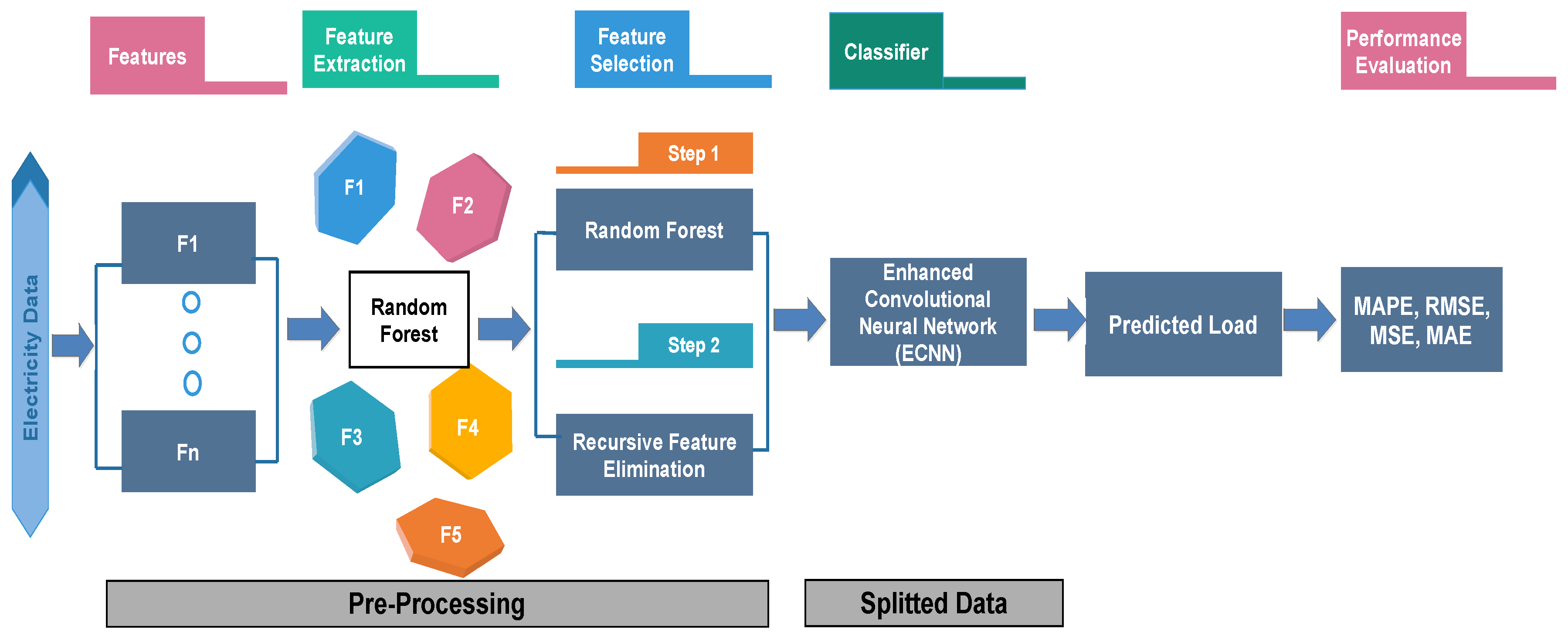
3.1. Electricity Load Forecasting Model
- Feature Extraction
- Feature Selection
- Load prediction using ECNN
- Performance evaluation
3.1.1. Data Source
3.1.2. Feature Extraction
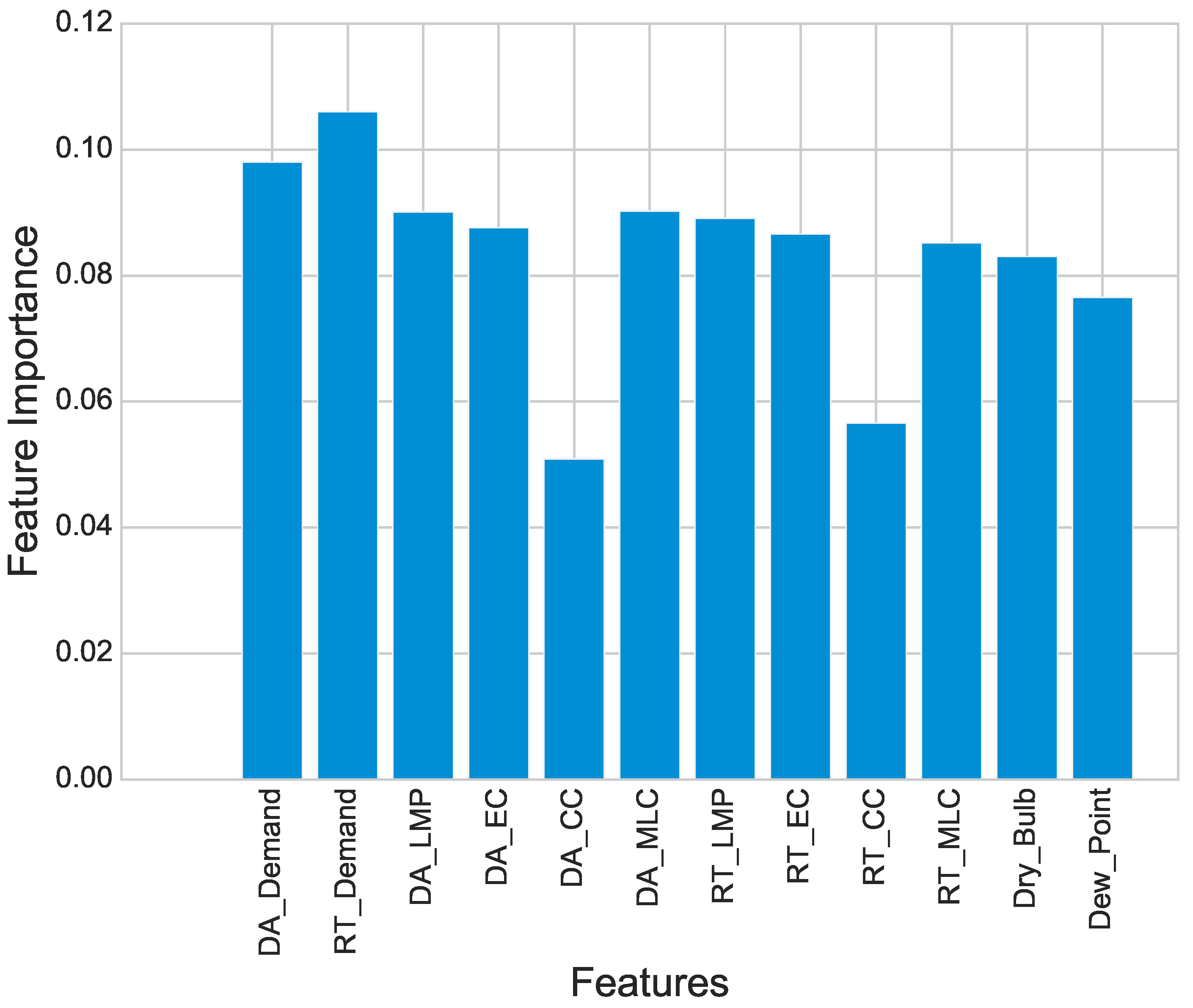
3.1.3. Feature Selection
3.1.4. ECNN
| Algorithm 1 Electricity Load Forecasting Model |
| Input: Electricity load data |
| /* Separate target from features */ |
| 1: X: features of data |
| 2: Y: target data |
| /* Split data into training and testing */ |
| 3: x_train, x_test, y_train, y_test = split(x, y); |
| 4: Combine_imp = DT − imp + XG − imp; |
| /* Calculate importance using Random Forest */ |
| 5: RF_imp = importance calculate by RF; |
| /* Feature extraction using RFE */ |
| 6: Selected_ feature = RFE(5, x_train, y_train); |
| /* Hybrid feature selection */ |
| 7: if (Combine_imp ≥ threshold And RFE == true) then |
| 8: Reserve feature; |
| 9: else |
| 10: Drop feature; |
| 11: end if |
| 12: Prediction using ESVM and ECNN with tuned parameters |
| 13: Compare predictions with y_test; |
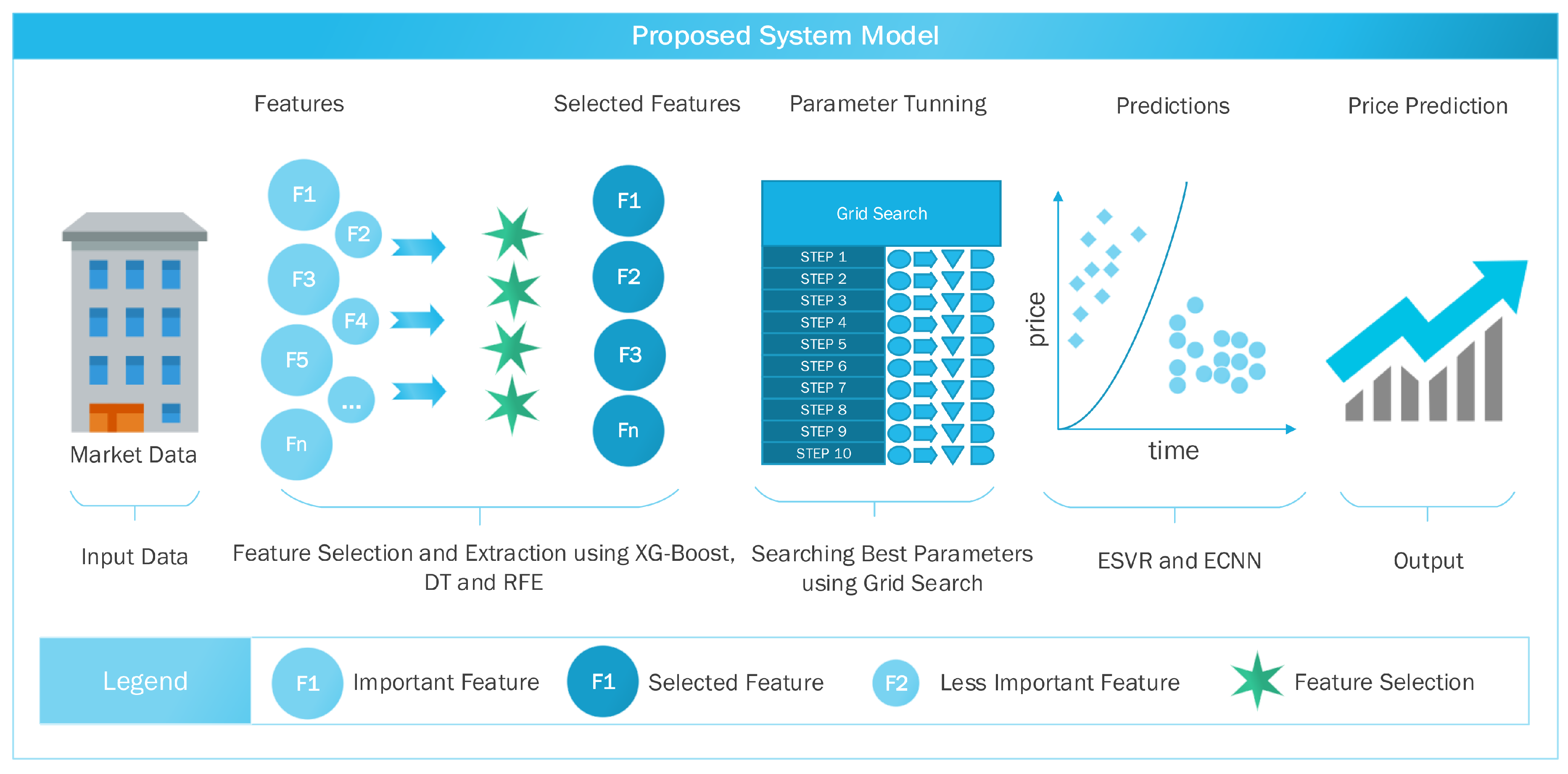
3.2. Electricity Price Forecasting Model
- Feature Selection
- Feature Extraction
- GS and cross-validation
- Price Prediction using ESVR and ECNN
3.2.1. Model Overview
3.2.2. Feature Extraction Using RFE
3.2.3. Feature Selection Using XG-Boost and DT
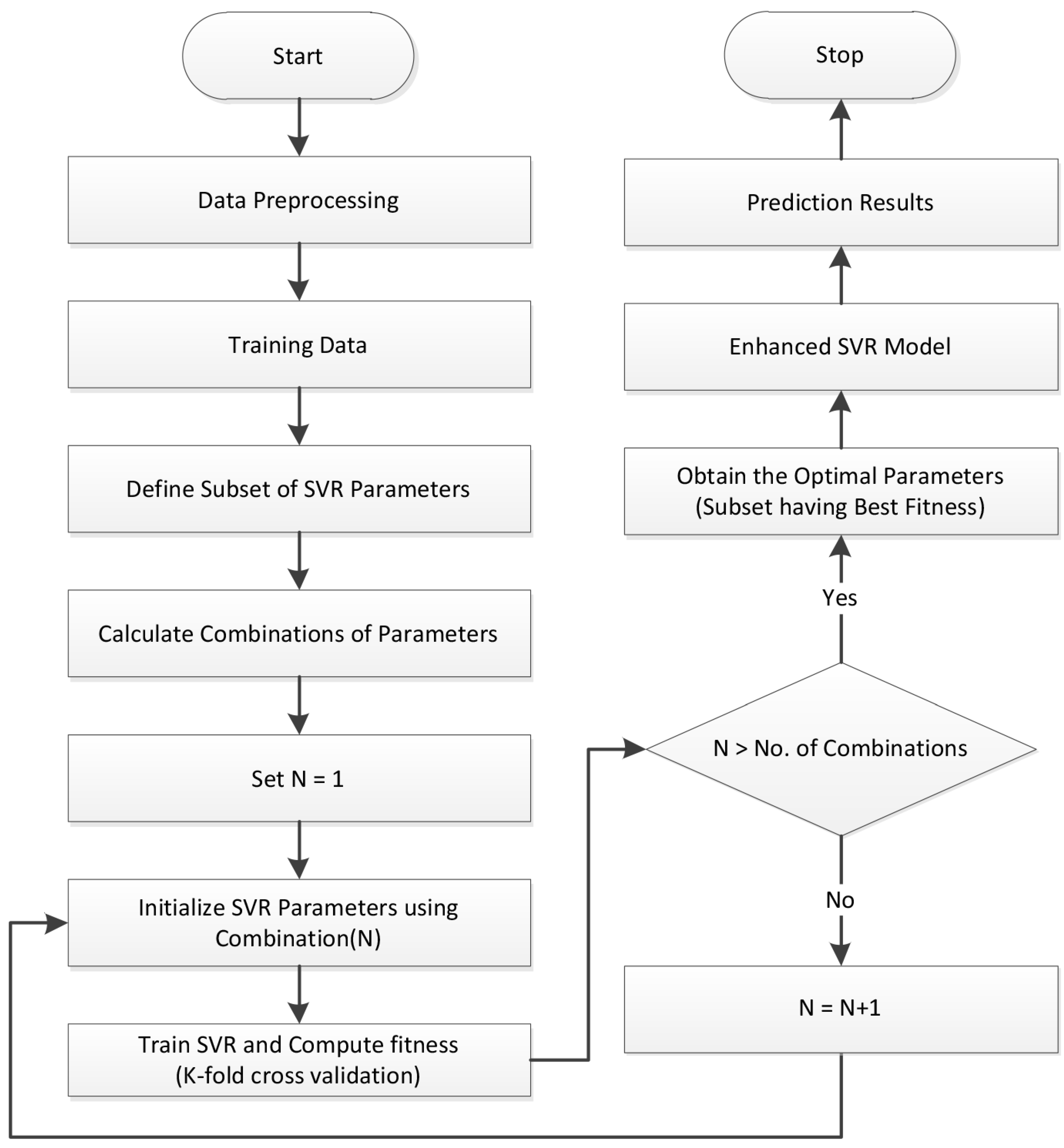
3.2.4. Tuning Hyper-Parameters and Cross-Validation
3.2.5. Electricity Price Forecasting
| Algorithm 2 Electricity Price Forecasting Model |
| Input: Electricity price data; |
| /* Separate target from features */ |
| 1: X: features of data; |
| 2: Y: target data; |
| /* Split data into training and testing */ |
| 3: x_train, x_test, y_train, y_test = train_test_split(x, y); |
| /* Feature extraction using RFE */ |
| 4: Selected_ feature = RFE(9, x_train, y_train); |
| /* Hybrid Feature Selection */ |
| 5: DT_imp = importance calculate by DT; C |
| 6: XG_imp = importance calculate by XG − boost; |
| 7: Combined_imp = DT_imp + XG_imp; |
| 8: if (combined_imp ≥ ϵ) then |
| 9: Reserve feature; |
| 10: else |
| 11: Drop feature; |
| 12: end if |
| 13: Grid Search for parameter tuning; |
| 14: Prediction using ESVR and ECNN with tuned parameters; |
| 15: Compare predicted price with actual price; |
4. Classifiers and Techniques
4.1. XG-Boost
4.2. DT
4.3. RFE
4.4. RF
4.5. Cross-Validation
4.6. GS
4.7. ESVR
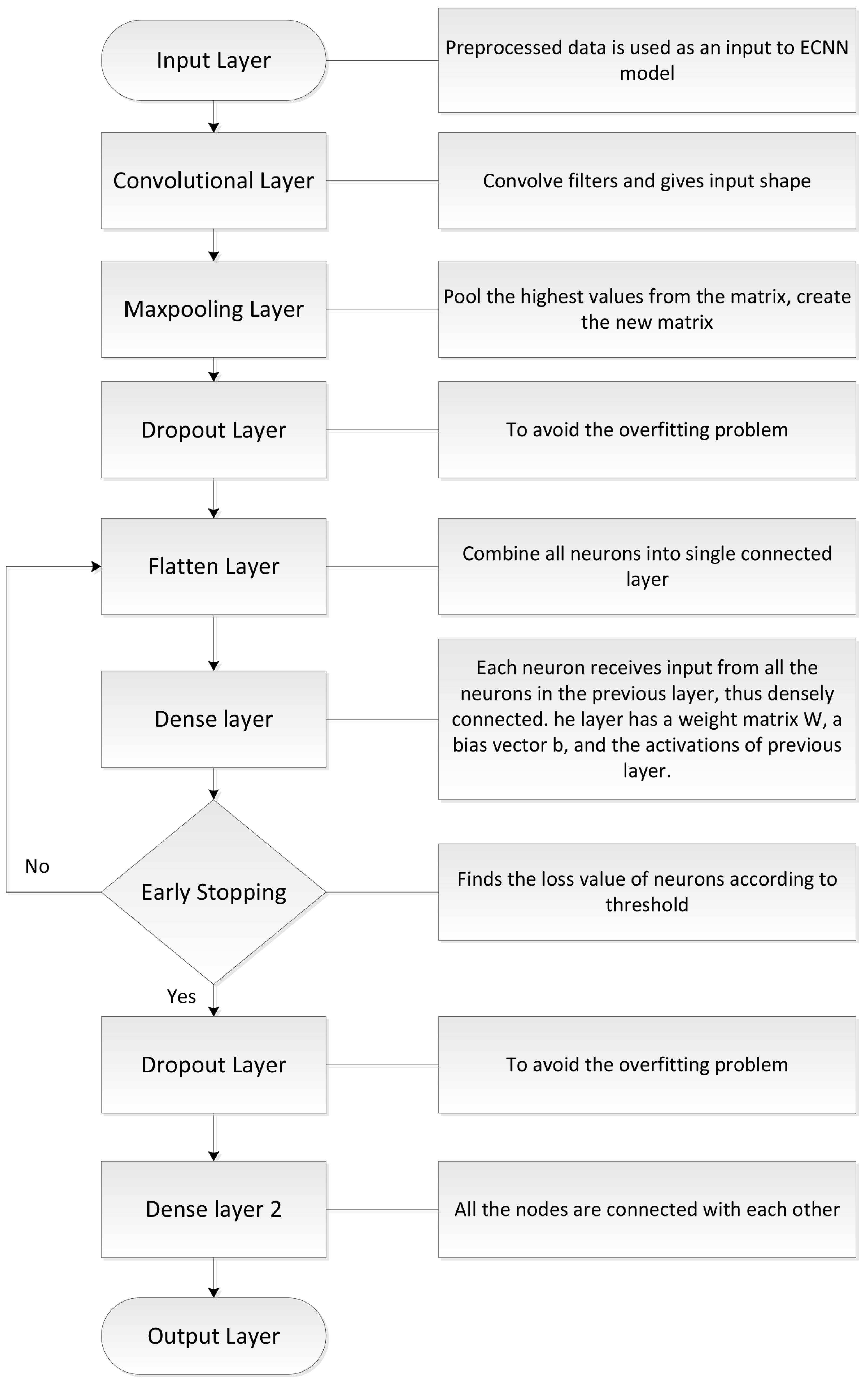
4.8. ECNN
4.8.1. Input Layer
4.8.2. Hidden Layer
4.8.3. Output Layer
4.8.4. Convolution Layer
4.8.5. Pooling Layer
- Max Pooling
- Average Pooling
- Sum Pooling
4.8.6. Activation Function
4.8.7. Work Flow of ECNN
4.9. Performance Evaluators
5. Simulation and Results
5.1. Simulation Environment
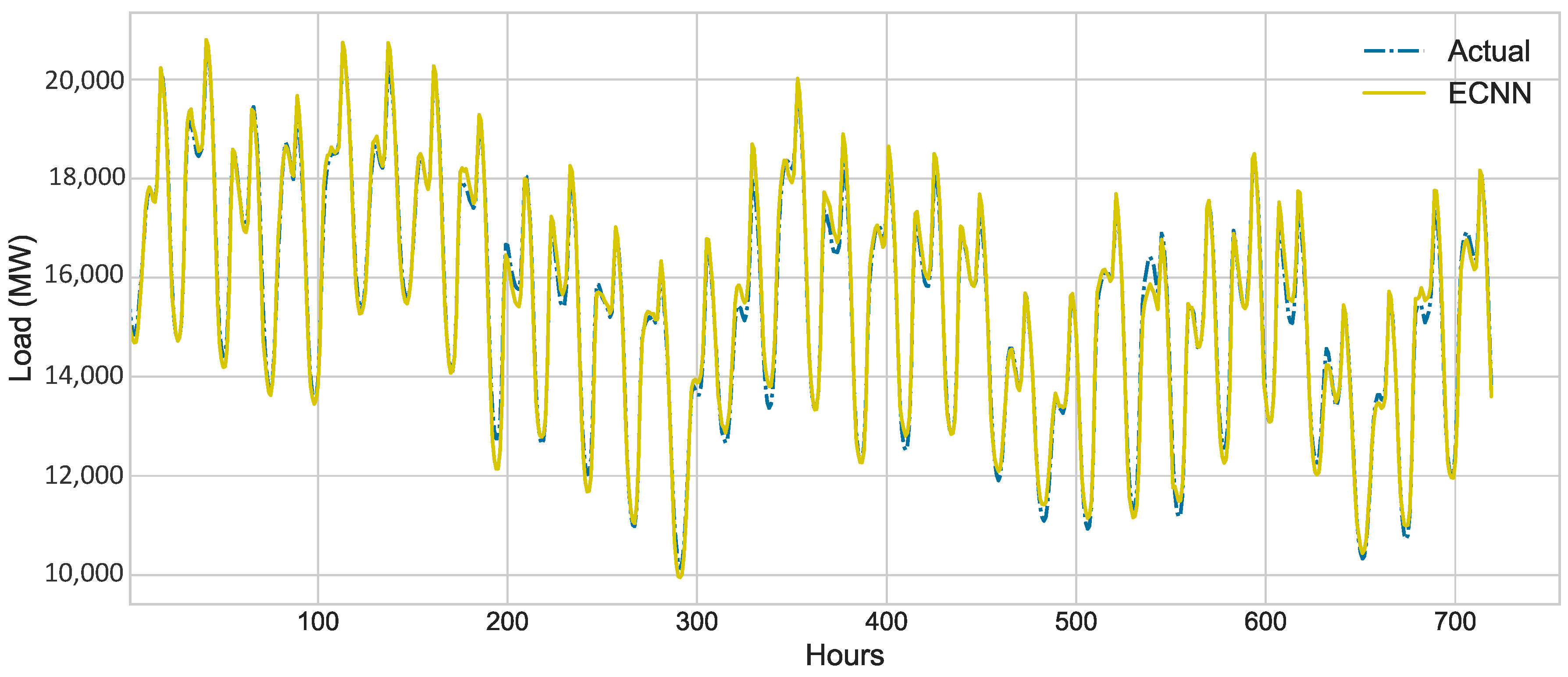
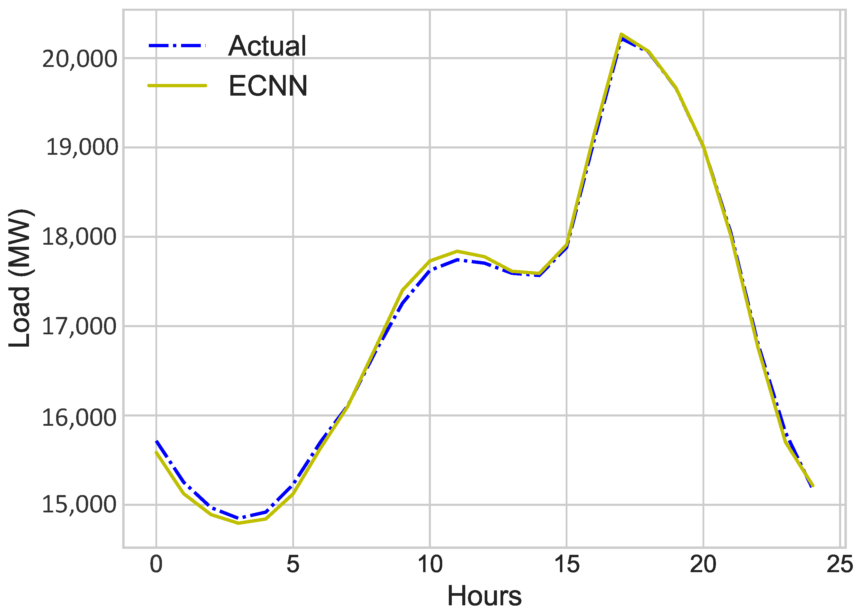
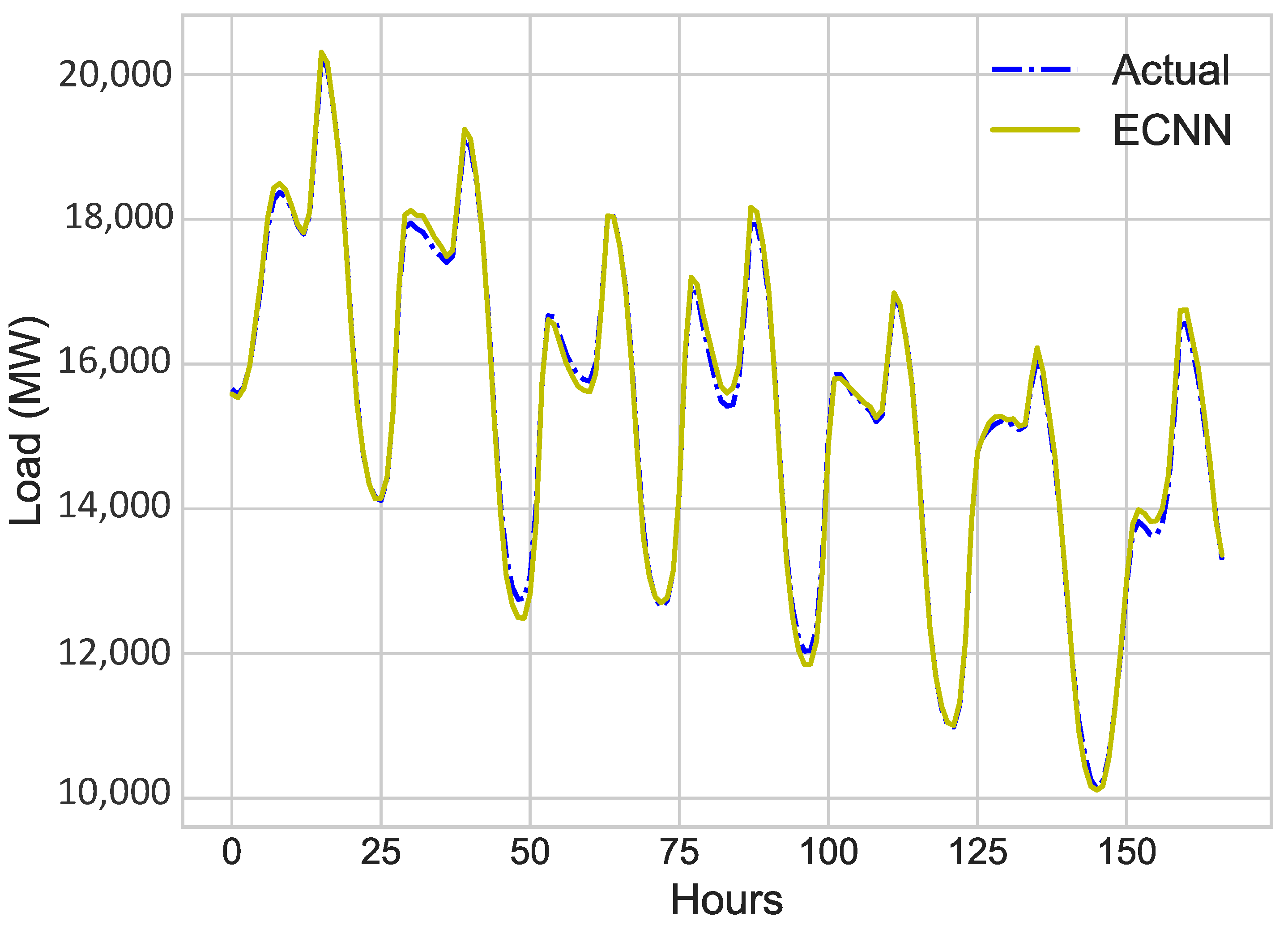
5.2. Results of Load Prediction Model
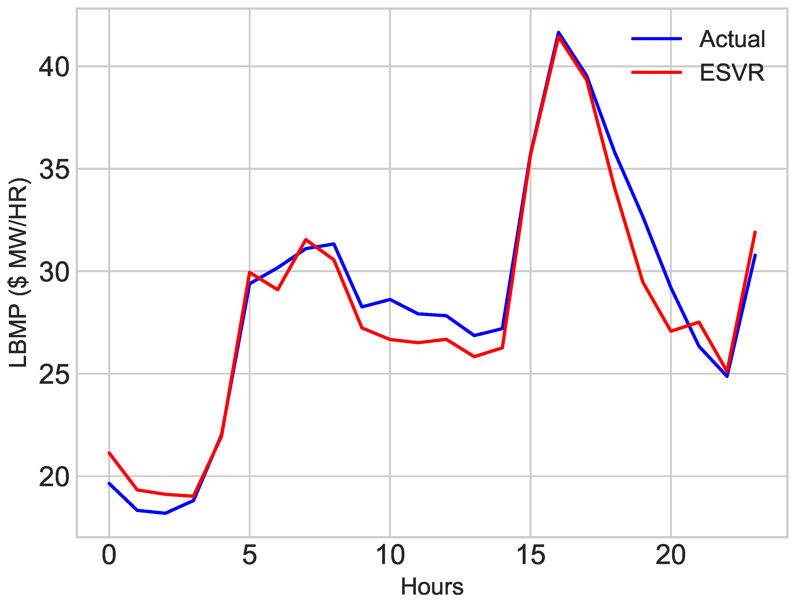
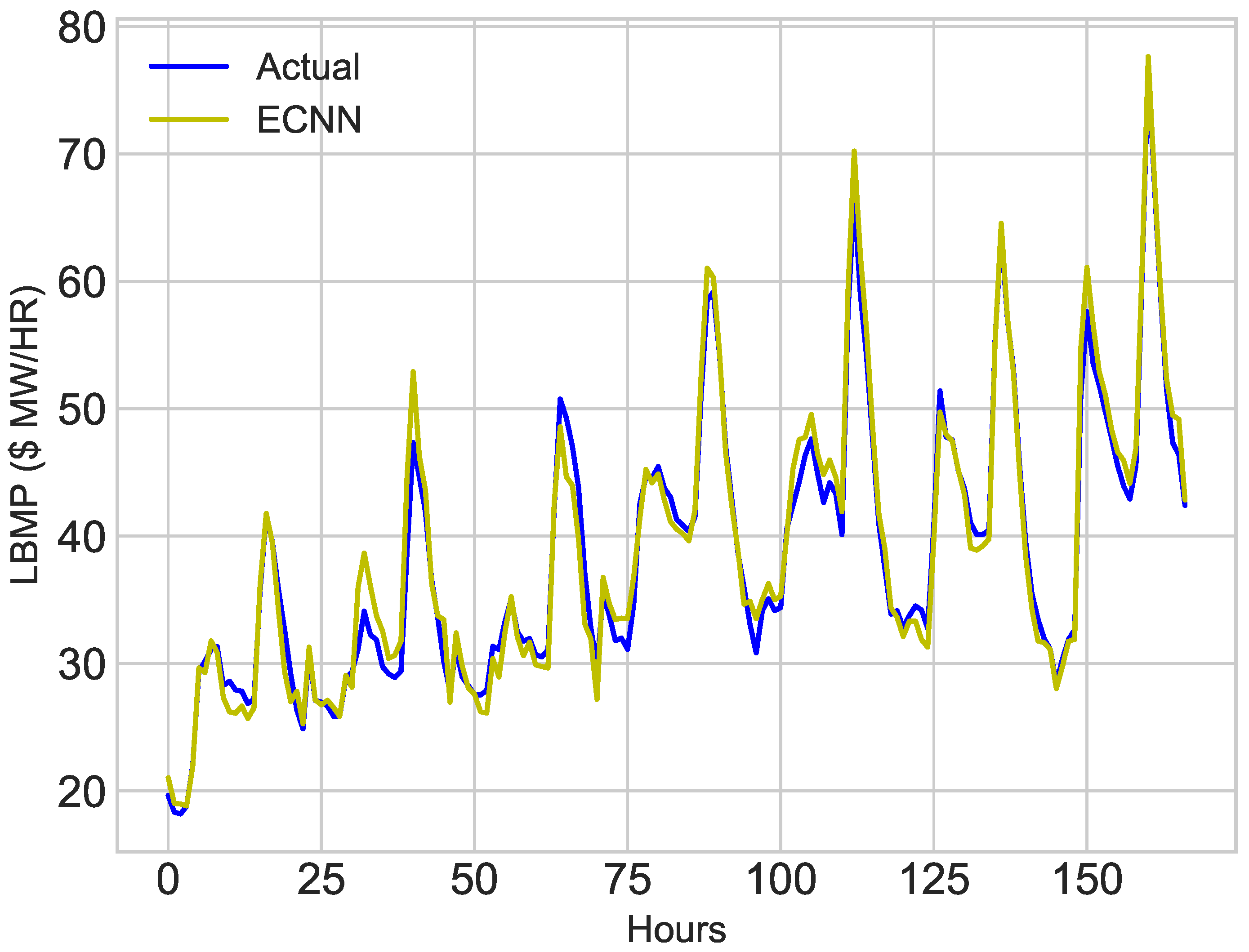
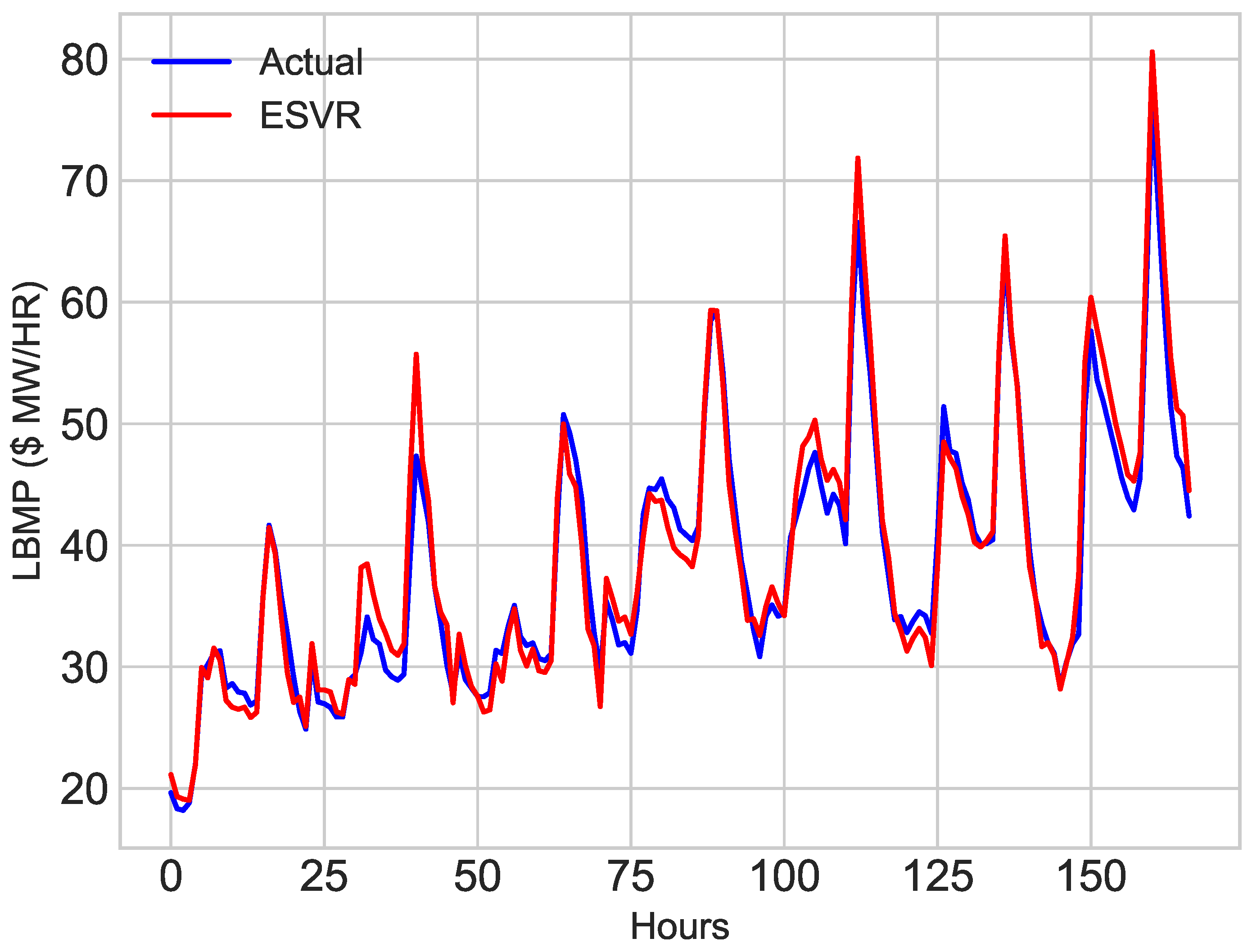
5.3. Results of Price Prediction Model
- Feature extraction using RFE
- Feature selection by combining the importance of attributes calculated by XG-boost and DT
- Parameter tuning using cross-validation and GS
- Prediction using ESVR and ECNN
- Results and Comparison with real data of January 2017
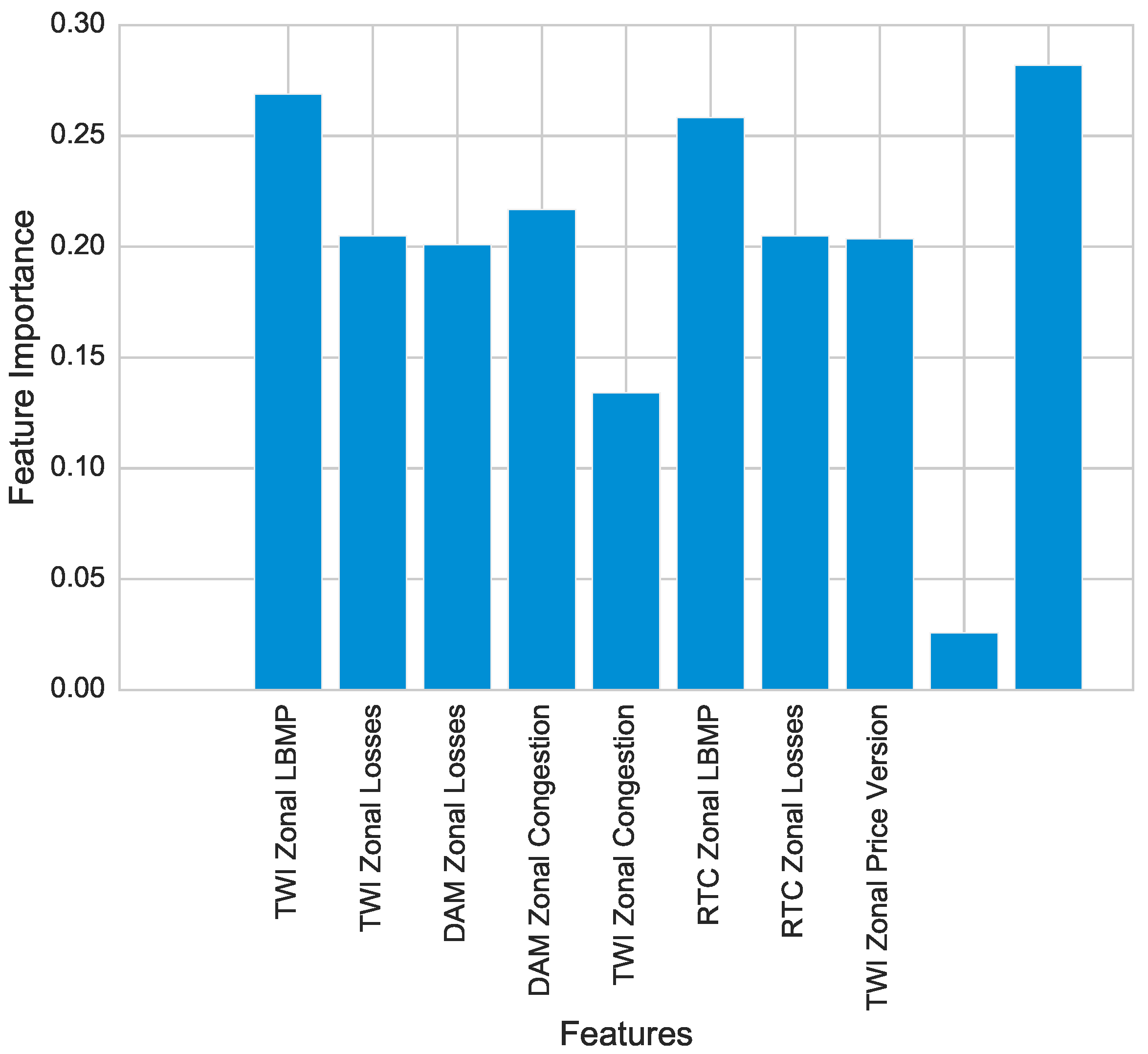
5.3.1. Feature Extraction
5.3.2. Feature Selection
5.3.3. Parameter Tuning and Cross-Validation
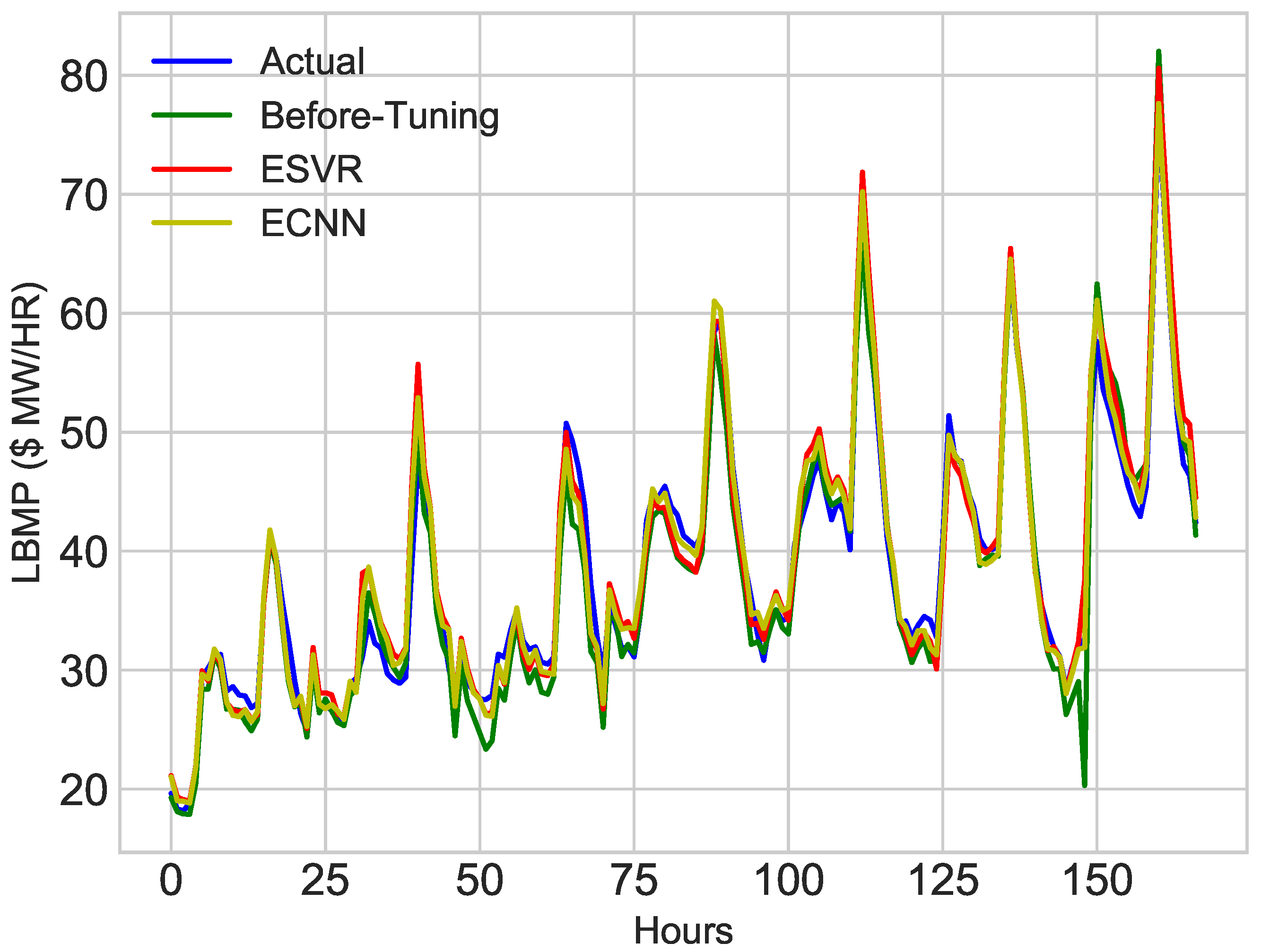
5.3.4. Price Prediction
5.4. Discussion of Results
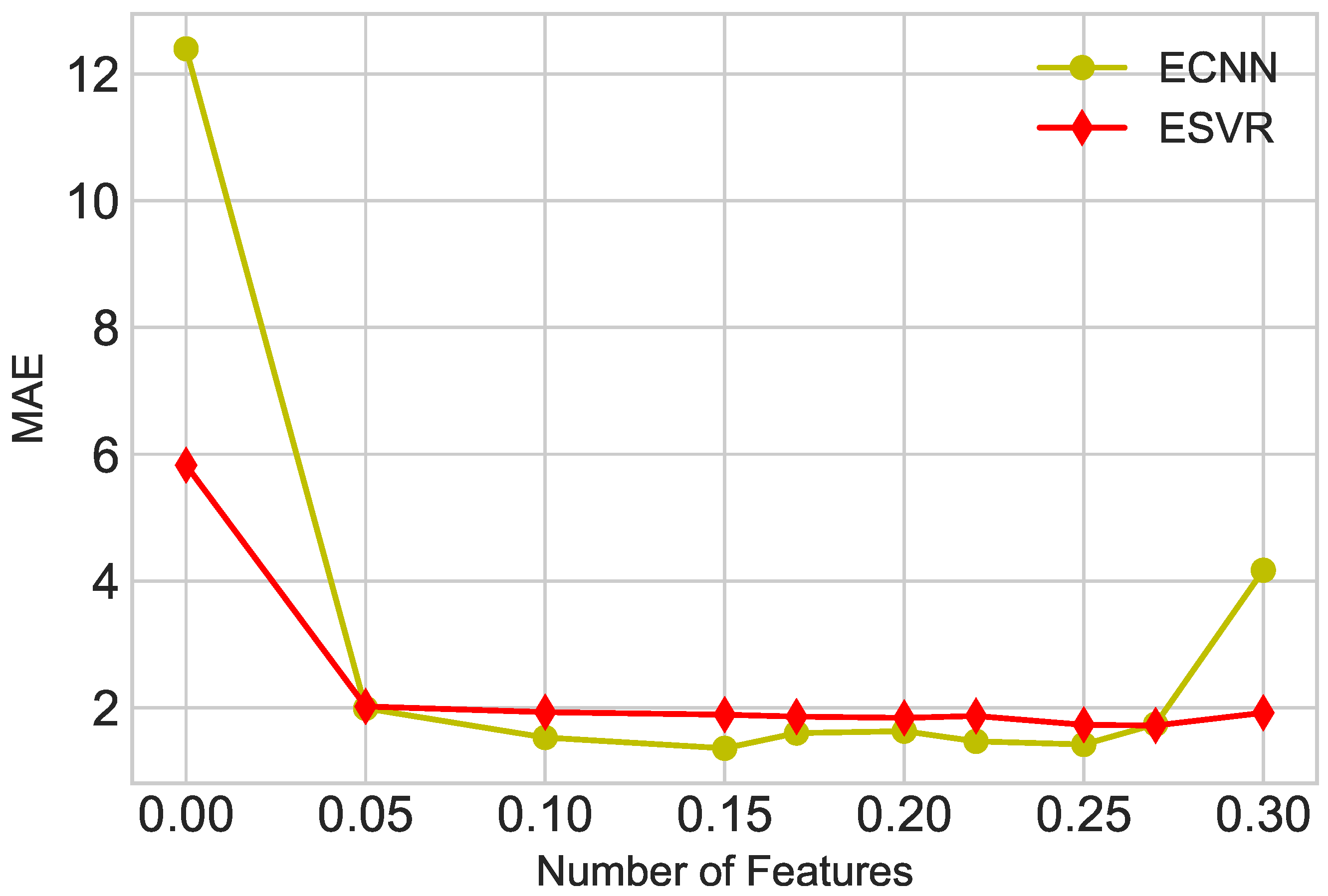
5.4.1. Effect of Hybrid Feature Selection Technique on Prediction
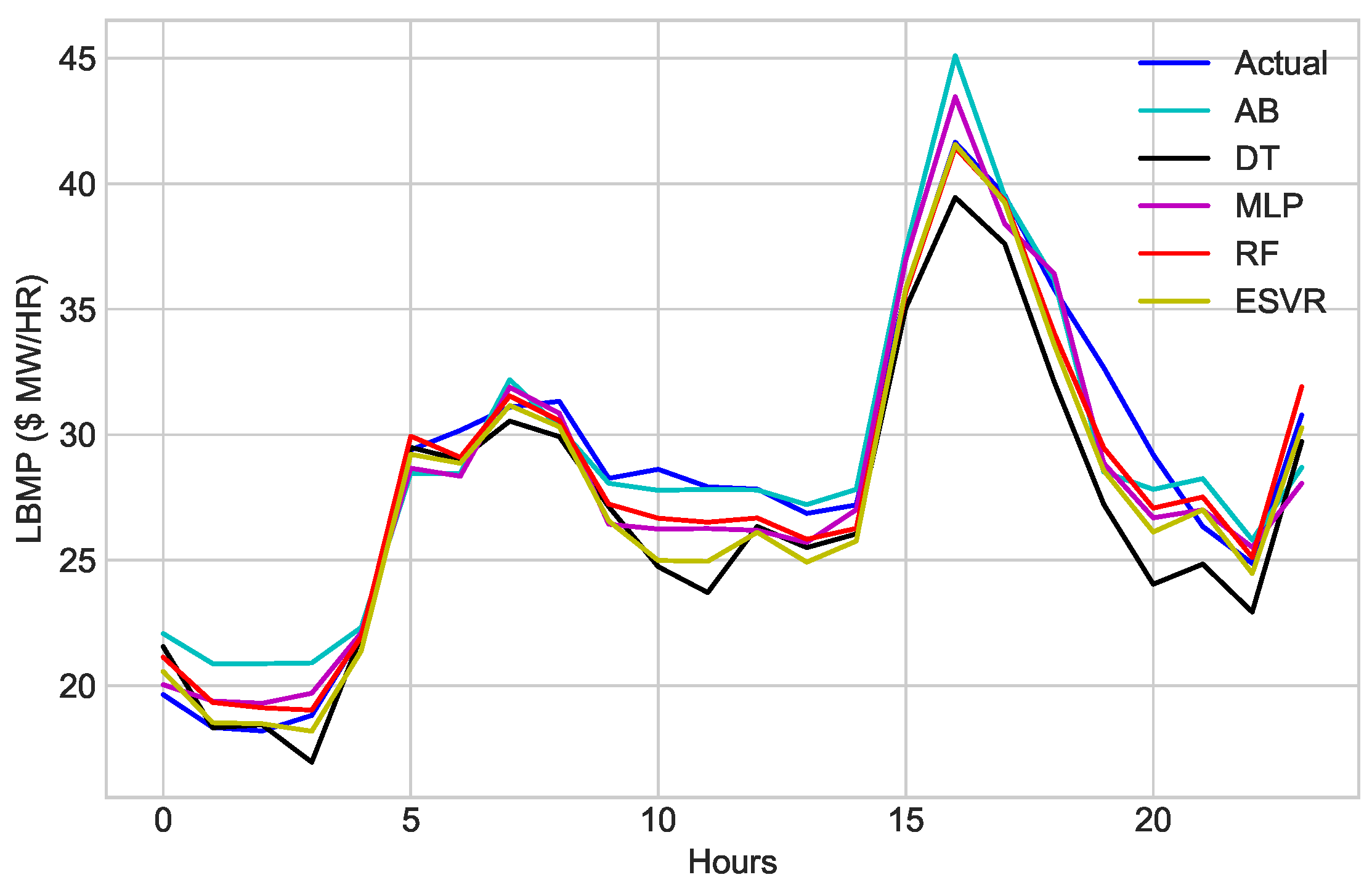
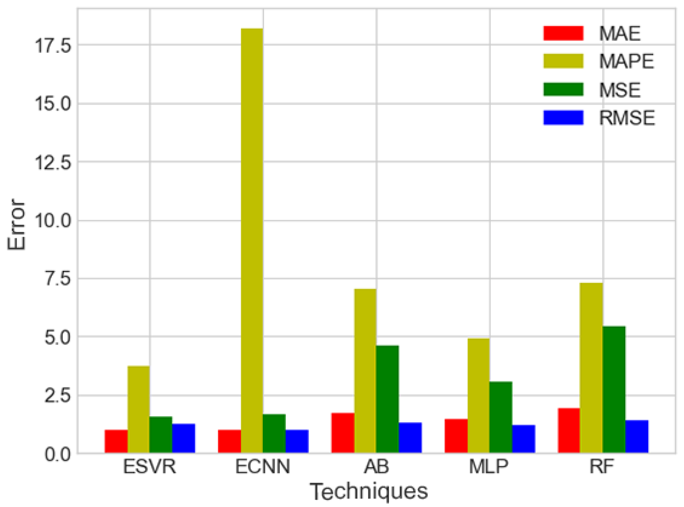
5.4.2. Comparison of Techniques
5.4.3. Effect of Dataset Size on Accuracy
6. Conclusions and Future Studies
Author Contributions
Conflicts of Interest
References
- Masip-Bruin, X.; Marin-Tordera, E.; Jukan, A.; Ren, G.J. Managing resources continuity from the edge to the cloud: Architecture and performance. Future Gener. Comput. Syst. 2018, 79, 777–785. [Google Scholar] [CrossRef]
- Osman, A.M. A novel big data analytics framework for smart cities. Future Gener. Comput. Syst. 2019, 91, 620–633. [Google Scholar] [CrossRef]
- Chen, X.-T.; Zhou, Y.-H.; Duan, W.; Tang, J.-B.; Guo, Y.-X. Design of intelligent Demand Side Management system respond to varieties of factors. In Proceedings of the 2010 China International Conference on Electricity Distribution (CICED), Nanjing, China, 13–16 September 2010; pp. 1–5. [Google Scholar]
- Bilalli, B.; Abelló, A.; Aluja-Banet, T.; Wrembel, R. Intelligent assistance for data pre-processing. Comput. Stand. Interfaces 2018, 57, 101–109. [Google Scholar] [CrossRef]
- Mohsenian-Rad, A.-H.; Leon-Garcia, A. Optimal residential load control with price prediction in real-time electricity pricing environments. IEEE Trans. Smart Grid 2010, 1, 120–133. [Google Scholar] [CrossRef]
- Chandrashekar, G.; Sahin, F. A survey on feature selection methods. Comput. Electr. Eng. 2017, 40, 16–28. [Google Scholar] [CrossRef]
- Erol-Kantarci, M.; Mouftah, H.T. Energy-efficient information and communication infrastructures in the smart grid: A survey on interactions and open issues. IEEE Commun. Surv. Tutor. 2015, 17, 179–197. [Google Scholar] [CrossRef]
- Wang, K.; Li, H.; Feng, Y.; Tian, G. Big data analytics for system stability evaluation strategy in the energy Internet. IEEE Trans. Ind. Inform. 2017, 13, 1969–1978. [Google Scholar] [CrossRef]
- Wang, K.; Ouyang, Z.; Krishnan, R.; Shu, L.; He, L. A game theory-based energy management system using price elasticity for smart grids. IEEE Trans. Ind. Inform. 2015, 11, 1607–1616. [Google Scholar] [CrossRef]
- Wang, H.Z.; Li, G.Q.; Wang, G.B.; Peng, J.C.; Jiang, H.; Liu, Y.T. Deep learning based ensemble approach for probabilistic wind power forecasting. Appl. Energy 2017, 188, 56–70. [Google Scholar] [CrossRef]
- Mosbah, H.; El-Hawary, M. Hourly electricity price forecasting for the next month using multilayer neural network. Can. J. Electr. Comput. Eng. 2016, 39, 283–291. [Google Scholar] [CrossRef]
- Hu, Q.; Zhang, R.; Zhou, Y. Transfer learning for short-term wind speed prediction with deep neural networks. Renew. Energy 2016, 85, 83–95. [Google Scholar] [CrossRef]
- Kuo, P.H.; Huang, C.J. An Electricity Price Forecasting Model by Hybrid Structured Deep Neural Networks. Sustainability 2018, 10, 1280. [Google Scholar] [CrossRef]
- Ugurlu, U.; Oksuz, I.; Tas, O. Electricity Price Forecasting Using Recurrent Neural Networks. Energies 2018, 11, 1255. [Google Scholar] [CrossRef]
- Eapen, R.R.; Simon, S.P. Performance Analysis of Combined Similar Day and Day Ahead Short Term Electrical Load Forecasting using Sequential Hybrid Neural Networks. IETE J. Res. 2018. [Google Scholar] [CrossRef]
- Zhang, X.; Wang, J.; Zhang, K. Short-term electric load forecasting based on singular spectrum analysis and support vector machine optimized by Cuckoo search algorithm. Electr. Power Syst. Res. 2017, 146, 270–285. [Google Scholar] [CrossRef]
- Patil, M.; Deshmukh, S.R.; Agrawal, R. Electric power price forecasting using data mining techniques. In Proceedings of the 2017 International Conference on Data Management, Analytics and Innovation (ICDMAI), Pune, India, 24–26 February 2017; pp. 217–223. [Google Scholar]
- Bouktif, S.; Fiaz, A.; Ouni, A.; Serhani, M. Optimal deep learning lstm model for electric load forecasting using feature selection and genetic algorithm: Comparison with machine learning approaches. Energies 2018, 11, 1636. [Google Scholar] [CrossRef]
- Ziming, M.A.; Zhong, H.; Le, X.I.; Qing, X.I.; Chongqing, K.A. Month ahead average daily electricity price profile forecasting based on a hybrid nonlinear regression and SVM model: An ERCOT case study. J. Mod. Power Syst. Clean Energy 2018, 6, 281–291. [Google Scholar]
- Lago, J.; de Ridder, F.; de Schutter, B. Forecasting spot electricity prices: Deep learning approaches and empirical comparison of traditional algorithms. Appl. Energy 2018, 221, 386–405. [Google Scholar] [CrossRef]
- Ghadimi, N.; Akbarimajd, A.; Shayeghi, H.; Abedinia, O. Two stage forecast engine with feature selection technique and improved meta-heuristic algorithm for electricity load forecasting. Energy 2018, 161, 130–142. [Google Scholar] [CrossRef]
- Jindal, A.; Singh, M.; Kumar, N. Consumption-Aware Data Analytical Demand Response Scheme for Peak Load Reduction in Smart Grid. IEEE Trans. Ind. Electron. 2018. [Google Scholar] [CrossRef]
- Chitsaz, H.; Zamani-Dehkordi, P.; Zareipour, H.; Parikh, P. Electricity price forecasting for operational scheduling of behind-the-meter storage systems. IEEE Trans. Smart Grid 2018, 9, 6612–6622. [Google Scholar] [CrossRef]
- Pérez-Chacón, R.; Luna-Romera, J.M.; Troncoso, A.; Martínez-Álvarez, F.; Riquelme, J.C. Big Data Analytics for Discovering Electricity Consumption Patterns in Smart Cities. Energies 2018, 11, 683. [Google Scholar] [CrossRef]
- Wang, Z.; Wang, Y.; Zeng, R.; Srinivasan, R.S.; Ahrentzen, S. Random Forest based hourly building energy prediction. Energy Build. 2018, 171, 11–25. [Google Scholar] [CrossRef]
- Lahouar, A.; Slama, J.B.H. Day-ahead load forecast using random forest and expert input selection. Energy Convers. Manag. 2015, 103, 1040–1051. [Google Scholar] [CrossRef]
- Wang, K.; Xu, C.; Zhang, Y.; Guo, S.; Zomaya, A. Robust big data analytics for electricity price forecasting in the smart grid. IEEE Trans. Big Data 2017. [Google Scholar] [CrossRef]
- Wang, L.; Zhang, Z.; Chen, J. Short-term electricity price forecasting with stacked denoising autoencoders. IEEE Trans. Power Syst. 2017, 32, 2673–2681. [Google Scholar] [CrossRef]
- Lago, J.; de Ridder, F.; Vrancx, P.; de Schutter, B. Forecasting day-ahead electricity prices in Europe: The importance of considering market integration. Appl. Energy 2018, 211, 890–903. [Google Scholar] [CrossRef]
- Raviv, E.; Bouwman, K.E.; van Dijk, D. Forecasting day-ahead electricity prices: Utilizing hourly prices. Energy Econ. 2015, 50, 227–239. [Google Scholar] [CrossRef]
- Mujeeb, S.; Javaid, N.; Akbar, M.; Khalid, R.; Nazeer, O.; Khan, M. Big Data Analytics for Price and Load Forecasting in Smart Grids. In International Conference on Broadband and Wireless Computing, Communication and Applications; Springer: Cham, Switzerland, 2018; pp. 77–87. [Google Scholar]
- Rafiei, M.; Niknam, T.; Khooban, M.-H. Probabilistic forecasting of hourly electricity price by generalization of ELM for usage in improved wavelet neural network. IEEE Trans. Ind. Inform. 2017, 13, 71–79. [Google Scholar] [CrossRef]
- Abedinia, O.; Amjady, N.; Zareipour, H. A new feature selection technique for load and price forecast of electrical power systems. IEEE Trans. Power Syst. 2017, 32, 62–74. [Google Scholar] [CrossRef]
- Ghasemi, A.; Shayeghi, H.; Moradzadeh, M.; Nooshyar, M. A novel hybrid algorithm for electricity price and load forecasting in smart grids with demand-side management. Appl. Energy 2016, 177, 40–59. [Google Scholar] [CrossRef]
- Shayeghi, H.; Ghasemi, A.; Moradzadeh, M.; Nooshyar, M. Simultaneous day-ahead forecasting of electricity price and load in smart grids. Energy Convers. Manag. 2015, 95, 371–384. [Google Scholar] [CrossRef]
- Keles, D.; Scelle, J.; Paraschiv, F.; Fichtner, W. Extended forecast methods for day-ahead electricity spot prices applying artificial neural networks. Appl. Energy 2016, 162, 218–230. [Google Scholar] [CrossRef]
- Wang, J.; Liu, F.; Song, Y.; Zhao, J. A novel model: Dynamic choice artificial neural network (DCANN) for an electricity price forecasting system. Appl. Soft Comput. 2016, 48, 281–297. [Google Scholar] [CrossRef]
- Varshney, H.; Sharma, A.; Kumar, R. A hybrid approach to price forecasting incorporating exogenous variables for a day ahead electricity market. In Proceedings of the IEEE International Conference on Power Electronics, Intelligent Control and Energy Systems (ICPEICES), Delhi, India, 4–6 July 2016; pp. 1–6. [Google Scholar]
- Fan, G.F.; Peng, L.L.; Hong, W.C. Short term load forecasting based on phase space reconstruction algorithm and bi-square kernel regression model. Appl. Energy 2018, 224, 13–33. [Google Scholar] [CrossRef]
- Dong, Y.; Zhang, Z.; Hong, W.-C. A Hybrid Seasonal Mechanism with a Chaotic Cuckoo Search Algorithm with a Support Vector Regression Model for Electric Load Forecasting. Energies 2018, 11, 1009. [Google Scholar] [CrossRef]
- Kai, C.; Li, H.; Xu, L.; Li, Y.; Jiang, T. Energy-Efficient Device-to-Device Communications for Green Smart Cities. IEEE Trans. Ind. Inform. 2018, 14, 1542–1551. [Google Scholar] [CrossRef]
- Kabalci, Y. A survey on smart metering and smart grid communication. Renew. Sustain. Energy Rev. 2016, 57, 302–318. [Google Scholar] [CrossRef]
- Mahmood, A.; Javaid, N.; Razzaq, S. A review of wireless communications for smart grid. Renew. Sustain. Energy Rev. 2015, 41, 248–260. [Google Scholar] [CrossRef]
- Zhou, L.; Wu, D.; Chen, J.; Dong, Z. Greening the smart cities Energy-efficient massive content delivery via D2D communications. IEEE Trans. Ind. Inform. 2018, 14, 1626–1634. [Google Scholar] [CrossRef]
- Available online: ISO-NE.com/isoexpress/web/reports/pricing/-/tree/zone-info (accessed on 7 October 2018).
- Fallah, S.N.; Deo, R.C.; Shojafar, M.; Conti, M.; Shamshirband, S. Computational Intelligence Approaches for Energy Load Forecasting in Smart Energy Management Grids: State of the Art, Future Challenges, and Research Directions. Energies 2018, 11, 596. [Google Scholar] [CrossRef]


| Technique(s) | Objectives | Achievement(s)/Data Source | Limitation(s) |
|---|---|---|---|
| [10] Multi Layer NN | Price Forecasting | Price prediction with acceptable accuracy | Loss rate and computational time is high |
| [13] HSDNN (Combination of LSTM and CNN) | Electricity price forecasting | PJM (half hour) | Computational time is high |
| [14] Gated Recurrent Units (GRU) | Price forecasting | Day ahead Turkish electricity market | Over-fitting problem is increased |
| [15] Back Propagation Neural Networks (BPNN) | Short-term Load forecasting | Day ahead Electric Reliability Council of Texas, USA | Complexity is increased |
| [16] CS-SSA-SVM | Load Forecasting | Half hourly, Hourly, Working day and Non-working day (New South Wales (Ten weeks data)) | Computational time is very high |
| [18] LSTM-RNN | Load Forecasting | Hourly and monthly Metropolitan France | The risk of over-fitting is not mitigated |
| [20] DNN, CNN, LSTM | Electricity price forecasting | Price forecasted | Redundancy is not removed and the effect of dataset size is not analyzed |
| [22] CC-DADR algorithm and UC-DADR | Reduce peak load and increase savings of consumer | Pennsylvania-New Jersey-Maryland Interconnection (PJM) | Less fault tolerance rate |
| [23] Battery based storage system | Price forecasting | Hourly data Ontario’s electricity market | The model is not robust and reliable |
| [24] Clustering Validity Indices (CVI’s) | Electricity consumption | Day ahead Eight building of University of Seoul, Korea | Computational time is very high |
| [25] Random Forest and Support Vector Regression (SVR) | Load Forecasting | Hourly Two educational buildings in North Central Florida | The model is not efficient and robust |
| [26] ANN and SVM | Load Forecasting | Day ahead Tunisian Power Company and PJM | Computational time is very high |
| [27] SVM, DCA, KPCA | Price forecasting | Forecast price and hybrid feature selection. | Dataset includes irrelevant features which increase computation overhead |
| [28] DNN, SVM | Short term electricity price forecasting | Comparison of different models and predict short term price. | Only suitable for specific scenario |
| [29] DNN | Price forecasting | Improve the accuracy and done feature selection by Bayesian Optimization | Redundancy and dimensionality reduction are not under consideration |
| [30] Multivariate Model | Hourly price prediction | Used multivariate model instead of univariate, reduce the risk of over-fitting | Performance of model is not compared with other techniques except uni-variate model |
| [31] DNN, LSTM | Price and Load Prediction | Predict both price and load | Price prediction is not accurate |
| [32] GELM | Hourly Price Prediction | Predict hourly price, Increase the speed of model using bootstraping techniques | Not work well for large datasets |
| [33] MI, IG | Feature Selection using Hybrid Algorithm | Improved accuracy by improving feature selection | Optimization of classifier is not considered |
| [34,35] LSSVM, QOABC | Price and Load Forecasting | Price and load forecasting along with conditional feature selection and modification in Artificial Bee Colony | Only suitable of their defined scenario |
| [36] ANN | Finding Best Parameters for ANN | Optimized parameter for ANN and price prediction | Overfitting problems are not considered |
| [37] DCANN | Day-ahead Price Forecasting | Price prediction and develop framework which choose neural network for scenario automatically. | Computational time is very high |
| [38] Hybrid NN model | Price Forecasting | Price forecasting and beat bench mark scheme. | Feature selection and extraction are neglected |
| Input | Filter | Output |
|---|---|---|
| Parameter Name | Parameter Values | Description |
|---|---|---|
| kernel | [‘linear’, ‘rbf’] | Kernel for Support Vector Machine |
| C | [3, 5, 10, 15, 20, 30] | C is a regularization parameter that controls the trade off between the achieving a low training error and a low testing error |
| gamma | [‘scale’, ‘gamma’, 10, 20, 30] | It is the inverse of the standard deviation, which is used as similarity measure between two points |
| epsilon | [0.2, 0.02, 0.002, 0.0002] | It is used to denote error margin, in terms of regressive functional loss |
| Parameter Name | Parameter Values | Desription |
|---|---|---|
| batch_size | [10, 20, 40, 50, 60] | The batch size defines the number of samples |
| epochs | [10, 30, 50, 70, 100, 150 | Number of iterations |
| learning_rate | [0.001, 0.01, 0.1, 0.2, 0.3] | Defined in the context of optimization, and minimizing the loss function of a neural network |
| activation | [‘softmax’, ‘relu’, ‘sigmoid’, ‘linear’] | Defines the output of a specific node |
| optimizer | [‘SGD’, ‘Adam’, ‘Adamax’, ‘Nadam’] | Update network weights iteratively to minimize the loss function |
| dropout_rate | [0.0, 0.1, 0.2, 0.3, 0.4, 0.5] | Dropout rate is a guidance for hidden layers to avoid over-fitting |
| Dataset | Technique | MAE | MAPE | MSE | RMSE |
|---|---|---|---|---|---|
| ISO-NE | SVR | 2.84 | 6.21 | 7.87 | 2.80 |
| ESVR | 2.11 | 5.3 | 6.72 | 2.59 | |
| CNN | 3.12 | 37.32 | 7.23 | 2.68 | |
| ECNN | 2.43 | 34.78 | 4.01 | 2.00 |
| Dataset | Technique | MAE | MAPE | MSE | RMSE |
|---|---|---|---|---|---|
| NYISO | SVR | 1.88 | 4.59 | 6.22 | 2.49 |
| ESVR | 1.78 | 4.2 | 5.23 | 2.28 | |
| CNN | 2.51 | 34.12 | 5.11 | 2.26 | |
| ECNN | 1.38 | 32.08 | 3.22 | 1.79 |
| Techniques | MAE | MAPE | MSE | RMSE |
|---|---|---|---|---|
| ESVR | 1.00 | 3.70 | 1.54 | 1.24 |
| ECNN | 0.99 | 18.18 | 1.64 | 0.99 |
| AdaBoost (AB) | 1.74 | 7.02 | 4.58 | 1.31 |
| Multi Layer Perceptron (MLP) | 1.43 | 4.90 | 3.06 | 1.19 |
| Random Forest (RF) | 1.91 | 7.31 | 5.40 | 1.38 |
| Dataset Size | No. of Records | Technique (s) | MAE | MAPE | MSE | RMSE |
|---|---|---|---|---|---|---|
| Small | 2000 | ECNN | 1.67 | 32.12 | 3.80 | 1.94 |
| ESVR | 1.78 | 4.60 | 4.78 | 2.18 | ||
| Medium | 4000 | ECNN | 1.65 | 32.39 | 4.92 | 2.21 |
| ESVR | 1.75 | 4.50 | 4.94 | 2.22 | ||
| Large | 6000 | ECNN | 1.46 | 18.17 | 3.54 | 1.88 |
| ESVR | 1.74 | 4.50 | 4.94 | 2.22 |
| Abbreviation(s) | Description(s) |
|---|---|
| ANN | Artificial Neural Network |
| BPNN | Back Propagation Neural Network |
| CNN | Convolutional Neural Network |
| DA | Data Analytic |
| DNN | Deep Neural Network |
| DR | Demand Response |
| DT | Decision Tree |
| FE | Feature Extraction |
| FS | Feature Selection |
| GCA | Grey Correlation Analysis |
| GELM | Generalize Extreme Learning Machine |
| KNN | K-Nearest Neighbor |
| KPCA | Kernel Principal Component Analysis |
| LR | Logistic Regression |
| LSTM | Long Short Term Memory |
| LTLF | Long-Term Load Forecasting |
| MAE | Mean Absolute Error |
| MAPE | Mean Absolute Percentage Error |
| MSE | Mean Square Error |
| STELF | Short-Term Electricity Load Forecasting |
| STLF | Short-Term Load Forecasting |
| MTLF | Medium-Term Load Forecasting |
| MLP | Multi Layer Perceptron |
| NYISO | New York Independent System Operator |
| RELU | Rectified Linear Unit |
| RF | Random Forest |
| RFE | Recursive Feature Elimination |
| RMSE | Root Mean Square Error |
| SDA | Stacked De-noising Auto-encoder |
| SG | Smart Grid |
| SM | Smart Meter |
| SVM | Support Vector Machine |
| SVR | Support Vector Regression |
| ESVR | Enhanced Support Vector Regression |
| TG | Traditional Grid |
© 2019 by the authors. Licensee MDPI, Basel, Switzerland. This article is an open access article distributed under the terms and conditions of the Creative Commons Attribution (CC BY) license (http://creativecommons.org/licenses/by/4.0/).
Share and Cite
Zahid, M.; Ahmed, F.; Javaid, N.; Abbasi, R.A.; Zainab Kazmi, H.S.; Javaid, A.; Bilal, M.; Akbar, M.; Ilahi, M. Electricity Price and Load Forecasting using Enhanced Convolutional Neural Network and Enhanced Support Vector Regression in Smart Grids. Electronics 2019, 8, 122. https://doi.org/10.3390/electronics8020122
Zahid M, Ahmed F, Javaid N, Abbasi RA, Zainab Kazmi HS, Javaid A, Bilal M, Akbar M, Ilahi M. Electricity Price and Load Forecasting using Enhanced Convolutional Neural Network and Enhanced Support Vector Regression in Smart Grids. Electronics. 2019; 8(2):122. https://doi.org/10.3390/electronics8020122
Chicago/Turabian StyleZahid, Maheen, Fahad Ahmed, Nadeem Javaid, Raza Abid Abbasi, Hafiza Syeda Zainab Kazmi, Atia Javaid, Muhammad Bilal, Mariam Akbar, and Manzoor Ilahi. 2019. "Electricity Price and Load Forecasting using Enhanced Convolutional Neural Network and Enhanced Support Vector Regression in Smart Grids" Electronics 8, no. 2: 122. https://doi.org/10.3390/electronics8020122
APA StyleZahid, M., Ahmed, F., Javaid, N., Abbasi, R. A., Zainab Kazmi, H. S., Javaid, A., Bilal, M., Akbar, M., & Ilahi, M. (2019). Electricity Price and Load Forecasting using Enhanced Convolutional Neural Network and Enhanced Support Vector Regression in Smart Grids. Electronics, 8(2), 122. https://doi.org/10.3390/electronics8020122