Angle of Arrival Passive Location Algorithm Based on Proximal Policy Optimization

Abstract

Location technology is playing an increasingly important role in urban life. Various active and passive wireless positioning technologies for mobile terminals have attracted research attention. However, positioning signals experience serious interference in high-density residential areas or in the interior of large buildings. The main type of interference is that caused by non-line-of-sight (NLOS) propagation. In this paper, we present a new method for optimizing the angle of arrival (AOA) measurement to obtain high accuracy location results based on proximal policy optimization (PPO). PPO is a new family of policy gradient methods for reinforcement learning, which can be used to adjust the sampling data under different environments using stochastic gradient ascent. Therefore, PPO can correct the NLOS propagation errors to produce a clear AOA measurement data set without building an offline fingerprinting database. Then, we used the least square method to calculate the location. The simulation result shows that the AOA passive location algorithm based on PPO produced more accurate location information.

1. Introduction

Location technology plays an important role in a variety of services, from mobile phone navigation in personal life, to search and rescue in natural disasters, and precision strikes in military applications. With the rapid development of location services, user demand is growing. Therefore, various active and passive wireless positioning technologies have attracted increasing attention and research [1,2,3].

In wireless positioning systems, positioning accuracy is the most fundamental index used to evaluate positioning performance. However, many factors affect the positioning accuracy, such as multipath propagation, multi-access interference, and non-line-of-sight (NLOS) propagation [4]. All these factors lead to errors in signal measurement information, resulting in decreased positioning accuracy. The main factor influencing positioning error is NLOS propagation [5]. NLOS propagation is caused by various obstacles between the mobile station (MS) and the base station (BS), interfering with the straight path of the signal wireless transmission, and the signal can only be transmitted through refraction or reflection, resulting in NLOS error. Compared with line-of-sight (LOS) propagation, signal propagation in a NLOS environment requires extra time and distance, resulting in signal arrival angle deviation and additional power loss. The NLOS error is generally only related to the environment in which the signal is propagated.

In wireless communication, many passive positioning technologies are used in research and applications, such as angle of arrival (AOA) [6], time of arrival (TOA) [7], and time difference of arrival (TDOA) [8]. Among them, the AOA does not require strict time synchronization, which is a necessary condition for TOA and TDOA. Therefore, the passive AOA location algorithm has wide and flexible application prospects. According to the current research situation, the AOA has a high positioning accuracy in the line of sight (LOS) environment [9]. However, like other localization methods, the accuracy of localization algorithms based on AOA methods are also greatly affected in NLOS environments [10,11].

When NLOS propagation occurs between the MS and BS, if the signal is not processed in advance and the measurement information transmitted by the signal NLOS is directly adopted for localization, localization accuracy is substantially reduced [12]. NLOS propagation problems exist in many application scenarios, such as urban environments, inside buildings, and in underground tunnels. Many studies have been conducted to eliminate NLOS effects, and various algorithms have been proposed to eliminate NLOS errors from different perspectives.

To mitigate the effects caused by NLOS, in [13,14,15] the researches have proposed some methods to correct the errors by adding anchors. Because of the need for additional nodes, these methods are not applicable to a wide range of outdoor environments. Shikur and Weber [16] presented a localization algorithm in NLOS environments using the Monte Carlo method. The limitation of the Monte Carlo method is that the average result is calculated through many cycles, which decreases the computational efficiency. Li et al. [17] proposed a hybrid TOA/AOA target localization method that can relax the stringent time synchronization requirement. The limitation is that, in the simulation environment, only Gaussian noise is introduced, which does not agree with the channel model in actual urban environments. Zhang et al. [18] proposed a novel TDOA/AOA wireless position scheme in the NLOS environment using Kalman filters to obtain a stable signal source, which reduced the location error. In [19,20], the researches proposed a geometrically model based single bounce circular. The model is just suitable for macro cell scenarios with large coverage where BS is very high relative to the detected object. The limitation of these methods [17,18,19] is that researchers only compensated for error in channel propagation models. They eliminated the error by changing the design of the receiver filter. These methods cannot be flexibly applied in the complex and changeable channel environment.

In the rapid deep learning development, some researchers used the iteration algorithm to mitigate the NLOS error. Wang et al. [21] proposed the mixed filter location method-based hierarchical voting. Before the traditional signal filtering, they carried out conditional detection and distance correction based hierarchical voting. This is a preliminary application of policy-based algorithm. Cheng et al. proposed an alternating optimization algorithm for localizing a mobile non-cooperative target using a wireless sensor network through AOA measurements in NLOS environments [22]. However, this algorithm is only suitable for centralized applications, and its computational complexity is largely dependent on the size of the network, so it cannot adapt to scenarios with high NLOS. An effective constrained weighted least squares (CWLS) algorithm was proposed [23]. This algorithm adopts the Newton iteration method that selects the least squares solution as the initial value to avoid premature convergence to the local minimum. Although this method is based on the pseudo-linear model, an appropriate initial guess is needed to ensure the convergence of the global optimal solution. This method provides a closed form solution for the estimation of emitter position and velocity. The method is based on the assumption that the location of the sensor is known, which is unrealistic. Wang et al. [24] proposed a fingerprinting system based on deep convolutional neural networks (DCNNs) for indoor localization. In this method, the AOA images are created and input to the DCNN to train the weights in the offline phase. The location result can be predicted based on the trained DCNN. Although the accuracy has been considerably improved, the calculation process still relies on pre-trained fingerprint database. A method based on deep neural network was proposed that allows a faster computation and lower memory usage [25]. However, this method improves the detection performance by learning a robust fingerprint representation in noisy and always changing environments without jointly addressing the issues related to noise and sparsity.

These researchers [22,23,24,25] adopted the iteration algorithm to reduce the error caused by the NLOS environment. However, these methods rely on a large amount of training data and an offline database, and the quality of training data determines the training effect of deep learning network, therefore, it is very important to obtain the best training database. For these problems, we present a new method to optimize the AOA based on deep reinforcement learning in a NLOS environment. Reinforcement learning can be broadly divided as value-based and policy-based. Different from the value-based algorithm, the policy-based algorithm is suitable for learning data with continuous time. Among the policy-based algorithms, trust domain strategy optimization (TRPO) and proximal strategy optimization (PPO) are typical strategy optimization methods. And PPO, which is evolved from TRPO, is a simpler and more general approach than TRPO [26,27]. So, we extend the state-of-the-art reinforcement learning algorithm, proximal policy optimization [28,29,30] to our error corrected training framework. The convergence problem of the policy gradient method is solved using the natural policy gradient method. In practice, however, the natural policy gradient involves a second-derivative matrix, which makes it non-scalable to large-scale problems. The computational complexity is too high for real tasks. PPO formalizes the constraint as a penalty in the target function instead of imposing a hard constraint. By avoiding constraints at all costs, a first-order optimizer, like gradient descent, can be used to optimize the target. Even though we sometimes violate the constraint, the effect is lessened and the calculation is much easier. The policy uses all the data gathered from parallel measurements for training. The parallel training framework not only considerably reduces the time cost of sample collection, but also enables the algorithm to be applied to various user equipment training in various scenarios.

The remainder of this paper is organized as follows: Section 2 describes the basic theory of multi-input multi-output (MIMO) system scenario, the AOA measurement in the MIMO, traditional AOA localization algorithm based on LS methods, the theory of proximal policy optimization, and the new AOA passive location algorithm for MIMO system based on PPO. Section 2 also gives the main flow chart of the proposed methods. Section 3 presents the simulated results. The simulation experiment includes the PPO training, the performance with different number of service base stations, cell radius, channel environment, and MS velocity. The experiment data is obtained from the AOA measurement error model and the actual NLOS communication scenario. The experimental results show that the algorithm proposed in this paper can produce high accuracy location results. Section 4 provides a summary, our conclusions, and recommendations for future research.

2. Materials and Methods

2.1. Scenarios

Assume that the base station has M transmit antennas, the mobile terminal has N receiver antennas, and the propagation path of the wireless channel has L propagation paths, then the receiver signal of the j receive antenna at time t can be defined as [31,32]:

$$y_j={\displaystyle \sum }_{i=1}^M{x}_i\left(t\right)h_{i,j}^l\left(t\right)+n_{i,j}\left(t\right)$$

(1)

where $h_{i,j}^l\left(t\right)$ is the channel model of i transmit antenna, j receive antenna at time t, $t_0$ is the delay time of multi-path. Each multi-path subchannel model of the of MIMO system can be defined as:

$$h_{i,j}^l\left(\tau -t\right)=h_{i,j}^l\left(t\right)\delta \left(\tau -t_0\right)$$

(2)

Equation (2) shows that in the non-ideal channel environment, the signal delay is always caused by refraction, scattering, reflection, and the influence of NLOS propagation. Therefore, the measurement of AOA between the mobile station(MS) and base station(BS_i) can be expressed as:

$${\alpha }_{i,j}={\alpha }_{0,i,j}+{\alpha }_{n,i,j}+{\alpha }_{e,i,j}$$

(3)

where ${\alpha }_{0,i,j}$ is the AOA value in the LOS environment, ${\alpha }_{n,i,j}$ is the environment error, ${\alpha }_{e,i,j}$ is the additional angle error caused by the NLOS, i is the number of transmitting antenna, and j is the number of receiving antenna.

2.2. AoA Passive Location Based on PPO

To solve this problem, we propose a new AOA passive location algorithm for a MIMO system based on PPO. PPO is used to modify the AOA measurement signal in the NLOS environment to reduce the NLOS error in the data. Then, the least squares (LS) method is used for location, which can effectively improve the positioning accuracy of the system. In this section, we introduce the new AOA passive location algorithm.

2.2.1. Traditional AOA Localization Algorithm

Assuming that the number of base stations is K, the position of MS is (x,y) and the position of BS_p is (x_p,y_p). The AOA values of each measured base station between ith transmission antenna and jth receiving antenna is ${\theta }_{p,i,j}$, which can be defined as:

$${\theta }_{p,i,j}=\arctan \frac{y-y_{p,i,j}}{x-x_{p,i,j}}$$

(4)

Then, we obtain the following formula:

$$tan\left({\theta }_{p,i,j}\right)x-y=tan\left({\theta }_{p,i,j}\right)x_{p,i,j}-y_{p,i,j}$$

(5)

When errors exist in the measured AOA data, the measurement error $\Psi$ can be defined as:

$$\Psi =h-G_{a}x$$

(6)

where $h$, $G_a$, $x$ are defined as follows:

$$h=\left[\begin{array}{c}{x}_1\tan {\theta }_{1,i,j}-y_1\\ x_2\tan {\theta }_{2,i,j}-y_2\\ ......\\ x_M\tan {\theta }_{M,i,j}-y_M\end{array}\right]$$

(7)

$$G_a=\left[\begin{array}{cc}\tan {\theta }_{1,i,j}& -1\\ \begin{array}{c}\tan {\theta }_{2,i,j}\\ ...\\ \tan {\theta }_{M,i,j}\end{array}& \begin{array}{c}-1\\ ...\\ -1\end{array}\end{array}\right]$$

(8)

$$x=\left[\begin{array}{c}x\\ y\end{array}\right]$$

(9)

Therefore, the MS position can be estimated by the LS algorithm as follows:

$$x={\left(G_a^T{G}_a\right)}^{-1}{G}_a^{T}h$$

(10)

The error of the LS algorithm of AOA is relatively small, which produces excellent performance in LOS environment. However, the error caused by the LS algorithm is relatively large in the NLOS environment.

2.2.2. Proximal Policy Optimization

The PPO algorithm proposed by OpenAI, which is a new policy gradient algorithm [27], algorithm has much lower implementation complexity than the trust region policy optimization (TRPO) algorithm [26]. The PPO algorithm mainly includes two implementation methods. The first PPO algorithm is realized by CPU simulation, and the second PPO algorithm is realized by GPU simulation. Its simulation speed is more than three times that of the first PPO algorithm. Compared with the traditional neural network algorithm, the PPO method achieves the best optimal balance in algorithm complexity, precision, and ease of implementation.

The basic PPO algorithm theory can be defined as:

$$J_{PPO}^{{\theta }^k}\left(\theta \right)\approx {\displaystyle \sum }_{\left(s_t,a_t\right)}min\left(\begin{array}{c}\frac{p_{\theta }(a_t|s_t)}{p_{{\theta }^k}(a_t|s_t)}{A}^{{\theta }^k}\left(s_t,a_t\right),\\ clip\left(\begin{array}{c}\frac{p_{\theta }(a_t|s_t)}{p_{{\theta }^k}(a_t|s_t)},\\ 1-\epsilon ,1+\epsilon \end{array}\right)\\ \times A^{{\theta }^k}\left(s_t,a_t\right)\end{array}\right)$$

(11)

where the output of the policy action in PPO is a set of discrete probability distribution, $p_{\theta }(a_t|s_t)$ is the probability value of the policy action in current state, and $p_{{\theta }^k}(a_t|s_t)$ is the probability value of the policy action in new state. Therefore, the ratio of the probability under the new and old policies can be defined as

$$R=\frac{p_{\theta }(a_t|s_t)}{p_{{\theta }^k}(a_t|s_t)}$$

(12)

where θ is the policy parameter.

Clip(*) is an amplitude limiting function; its maximum value is $1+\epsilon$,the minimum value $1-\epsilon$. $\epsilon$ is a hyper parameter, the range is always from 0.1 to 0.2, which reflects the difference between the new and old policies. The function of trust zone update can be implemented using this objective function, which is compatible with random gradient descent. The equation of Clip(*) is defined as follows:

$$clip\left(\begin{array}{c}\frac{p_{\theta }(a_t|s_t)}{p_{{\theta }^k}(a_t|s_t)},\\ 1-\epsilon ,1+\epsilon \end{array}\right)=\{\begin{array}{c}1-\epsilon ,\frac{p_{\theta }(a_t|s_t)}{p_{{\theta }^k}(a_t|s_t)}\le 1-\epsilon \\ 1+\epsilon ,\frac{p_{\theta }(a_t|s_t)}{p_{{\theta }^k}(a_t|s_t)}\ge 1-\epsilon \\ \frac{p_{\theta }(a_t|s_t)}{p_{{\theta }^k}(a_t|s_t)},other\end{array}$$

(13)

where $A^{{\theta }^k}\left(s_t,a_t\right)$ is the estimated advantage at time t. When $A^{{\theta }^k}\left(s_t,a_t\right)>0$, the state action of the PPO algorithm has a positive advantage, so the contribution of Equation (11) to the target can be simplified as:

$$J_{PPO,1}^{{\theta }^k}\left(\theta \right)\approx {\displaystyle \sum }_{\left(s_t,a_t\right)}min\left(\frac{p_{\theta }(a_t|s_t)}{p_{{\theta }^k}(a_t|s_t)},1+\epsilon \right)A^{{\theta }^k}\left(s_t,a_t\right)$$

(14)

At this time, due to the advantage being positive, the target will increase. When $p_{\theta }(a_t|s_t)>\left(1+\epsilon \right)p_{{\theta }^k}(a_t|s_t)$, starting from the minimum value, the value of Equation (14) can reach the upper limit $\left(1+\epsilon \right)A^{{\theta }^k}\left(s_t,a_t\right)$, which ensures that the new strategy is not too different from the old strategy. Then, for this state, the algorithm encourages new strategies to increase the corresponding probability of action as shown in Figure 1.

When $A^{{\theta }^k}\left(s_t,a_t\right)\le 0$, the state action of the OPP algorithm has a negative advantage, so the contribution of Equation (11) to the target can be simplified as:

$$J_{PPO,2}^{{\theta }^k}\left(\theta \right)\approx {\displaystyle \sum }_{\left(s_t,a_t\right)}min\left(\frac{p_{\theta }(a_t|s_t)}{p_{{\theta }^k}(a_t|s_t)},1-\epsilon \right)A^{{\theta }^k}\left(s_t,a_t\right)$$

(15)

At this time, because the advantage is negative, therefore, the target will decrease. When $p_{\theta }(a_t|s_t)<\left(1-\epsilon \right)p_{{\theta }^k}(a_t|s_t)$, starting from the maximum value, the value of Equation (15) can reach the lower limit $\left(1-\epsilon \right)A^{{\theta }^k}\left(s_t,a_t\right)$, which will ensure that the new strategy is not far from the old strategy (which is shown in Figure 2).

2.2.3. Amendment of AOA Measurement Based on PPO

Here, we use the PPO method to correct the NLOS error and the measurement error, which make the AOA value to close the real value. The operation process is as follows:

Step 1: Sample the N₁ set of AOA measurement value $\left\{NAO{A}_i,i=1,...,N_1\right\}$ under the NLOS environment. Sample the N₂ set of the AOA measurement value $\left\{AO{A}_i,i=1,...,N_1\right\}$ without any interference under the LOS environment. Take the $NAO{A}_i$ as the PPO training data and take the $AO{A}_i$ as the PPO training target data. The relationship between $NAO{A}_i$ and $AO{A}_i$ can be defined as:

$$NAO{A}_i=AO{A}_i+n_i+{\alpha }_{e,i}$$

(16)

where $n_i$ is system measurement error and ${\alpha }_{e,i}$ is the additional angle error caused by NLOS.

Step 2: PPO Training. Assume that $NAO{A}_i$ and $AO{A}_i$ are sampled from ten related base stations. Therefore, the input of PPO can be represented as:

$$P=\left[NAO{A}_{i,1},NAO{A}_{i,6},...,NAO{A}_{i,10}\right].$$

(17)

The output of PPO can be expressed as:

$$T=\left[AO{A}_{i,1},AO{A}_{i,6},...,AO{A}_{i,10}\right]$$

(18)

The variable P represents the training input data of PPO. The variable T represents the training target data of PPO.

The PPO training process is as follows. Figure 3 shows that the input unit produces a feedback action when the environmental state is perceived through the P data, then the environment can send a reinforcement signal r(t) to the PPO unit. Simultaneously, the PPO unit updates the knowledge database of the policy module. The actor module selects a certain action a(t) in the range of ε according to the current state P(t) and reinforcement information r(t), and then acts on the current environment to change the environment. In this paper, the certain action a(t) is the value, which can make the AOA value is as close to the real value as possible. The state P(t) is the value, which expresses the current AOA value, and the reinforcement information r(t) can control the PPO model whether the AOA value should be corrected or not. After multiple iterations of the actor and critic, we can obtain an optimal policy.

According to PPO theory, when the advantage of the state-action pair is positive, the PPO increases the amendment value of the AOA measurement. When the advantage of the state–action pair is negative, the PPO decreases the amendment value of AOA measurement:

$${\xi }_i=\{\begin{array}{c}{\xi }_i+{\gamma }_i,A^{{\theta }^k}\left(s_t,a_t\right)>0\\ {\xi }_i,A^{{\theta }^k}\left(s_t,a_t\right)=0\\ {\xi }_i-{\gamma }_i,A^{{\theta }^k}\left(s_t,a_t\right)<0\end{array}$$

(19)

where ${\xi }_i$ is the amendment value and ${\gamma }_i$ is the increase or decrease part of ${\xi }_i$. After several iterations, the action $a_t$ ensures the output P of the environment module is close to the value of T.

A trained PPO model is used to correct the measurement data of AOA. The revised AOA is used to estimate the position using Equation (10).

In the process, the PPO policy update can be defined as:

$${\theta }_{k+1}=\arg \underset{\theta }{\max }\underset{s,a~{\pi }_{{\theta }_k}}{E}\left[J_{PPO}^{{\theta }^k}\left(\theta \right)\right].$$

(20)

Finally, the PPO training process is finished.

According to the above introduction, the main flow of the AOA passive location algorithm for a MIMO system based on PPO is shown in Figure 4.

In summary, the training PPO model can modify the AOA measurement data, and then reduce the NLOS error of the AOA measurement value.

3. Experiment

In this study, the proposed AOA passive location algorithm for an MIMO system based on PPO was simulated to estimate the location accuracy.

In this experiment, 1000 MS were located with uniform distribution as the target data. The training analog measurement data were obtained according to the AOA measurement error model, the testing analog measurement data includes two parts, the first part of testing data were obtained according to the AOA measurement error model, the second part of testing data were obtained from real data in the actual NLOS communication scenario.

We used the COST259 model to create the scenario and determined the additional delay error caused by NLOS, which follows Gaussian distribution [33]. The AOA error follows Gauss distribution with a mean value of 0 and standard deviation of 0.04 rad/s. The delay error caused by NLOS obeys the general COST259 urban model.

3.1. Simulation Experiment Parameters

The parameters of the simulation scenarios are listed in

Table 1. Scenario simulation parameters.

No.	Performance Index	Value
1	Number of multi-input multi-output (MIMO) transmitting antennas	4
2	Number of MIMO receiving antennas	4
3	Number of service base stations	4
4	Position of service base stations	(0,0)
5	Number of Moblie Station (MS)	1000
6	Initial position of MS	Random distribution in 400 × 400 region
8	Observation period	1 s
9	Cellradius	2500 m
10	Distribution of AOA error	Gaussian(0,0.04)
11	Channel model	COST259 model
12	Number of training data	10000 sets of training data from COST259 model
13	Number of testing data	1000 sets of testing data from actual NLOS scenario
-	-	5000 sets of testing data from COST259 model
14	Number of Monte Carlo cycles	1000

and the PPO methods parameters are shown in

Table 2. PPO simulation parameters.

No.	Performance Index	Value
1	PPO training iteration number	5000
2	Actor learning rate	0.0001
3	Critic learning rate	0.0002
4	Actor iteration number	10
5	Critic iteration number	10

. The system performance of the algorithm proposed in this paper was simulated and analyzed.

The PPO training iteration number affects the training performance of PPO, when if iteration number is small, the training performance of PPO will be bad, otherwise the training performance of PPO will be better. Considering the training performance and training time of PPO, the number of iterations is 5000 in this paper. The Actor and Critic learning rate affects the learning efficiency of PPO, lower learning rate will cause pool learning efficiency, while the large learning rate will cause training can’t converge. Considering the efficiency and convergence of PPO training, we set Actor and Critic learning rate is 0.0001 and 0.0002 respectively.

We placed 7 base stations on the campus of Beijing university of posts and telecommunications for real NLOS data collection, as shown in Figure 4:

The proposed method has been validated utilizing a dual channel receiver using Universal Software Radio Peripheral (USRP) X310 as shown in Figure 5. The USRP X310 contains 2Tx and 2Rx ports with fully coherent 2 × 2 MIMO capabilities. The coherency between the Rx ports is an essential feature for extracting accurate phase difference between the received signals. Moreover, the USRP X310 covers RF frequencies from DC to 6GHz with a maximum ADC sample rate 200MS/s. Thus the USRP X310 was an ideal candidate for this project. The USRP X310 was configured with the GNU radio companion (GRC) interface. GRC is a graphical user interface to build GNU radio flow graphs or the software circuits. The GNU radio flow graph enables the SDR card to receive signals from the antennas, spectrally isolate them, and then calculate the phase difference between the received signals. Aziz [34] have completed the AOA data acquisition model based on USRP device. According to his model, we completed the collection of the original data and used it for the subsequent PPO algorithm verification.

3.2. Simulation and Experimental Analysis

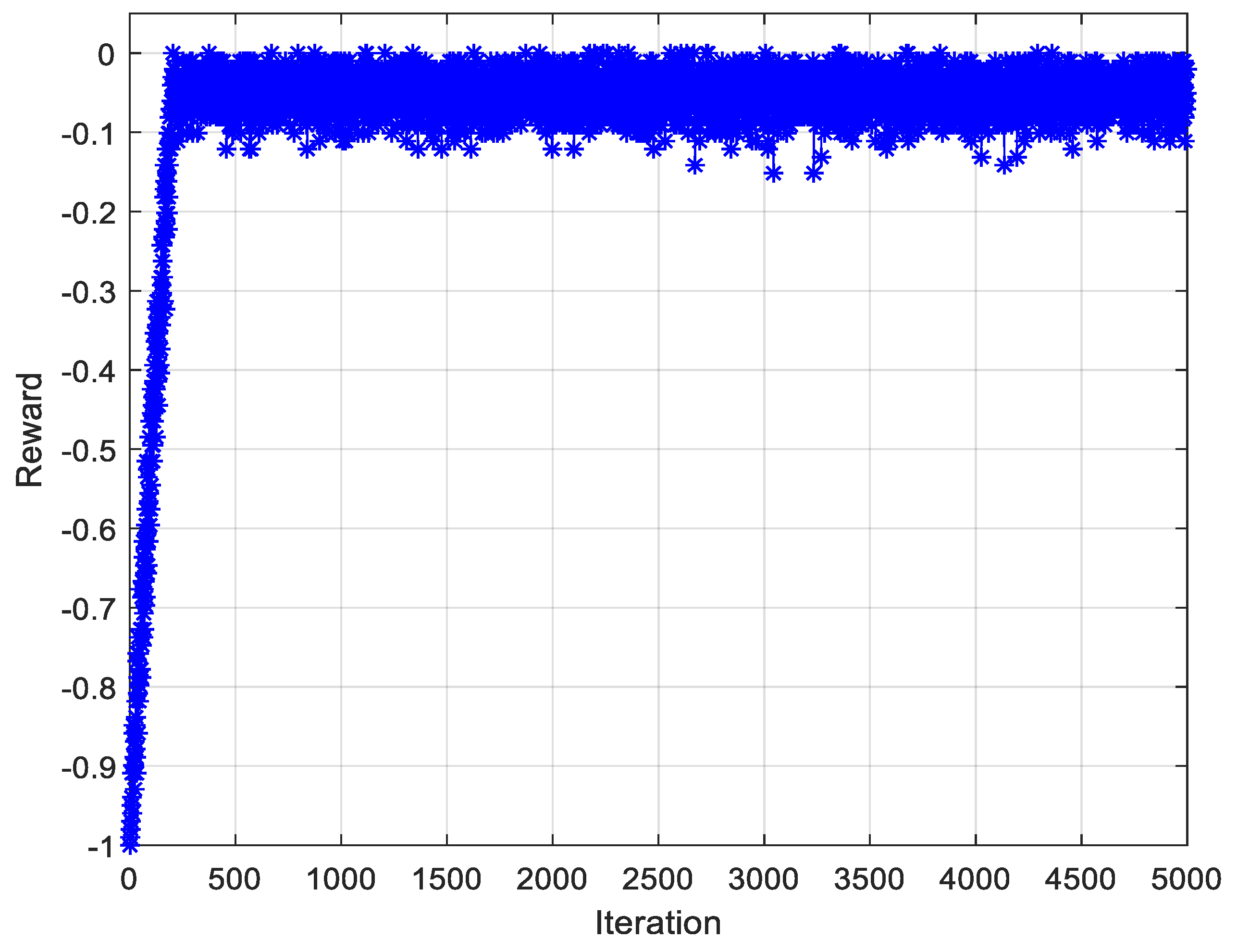
According to the basic flow chart in Figure 6 and the simulation parameters in Table 1 and Table 2, we analyzed the influence of position performance, including the iteration times of PPO training, the cell radius, the number of service base stations, the number of MIMO antennas, the channel environment, the MS velocity, and the number of training measurement data.

The measurement error ${\phi }_i$ of AOA measurement data obeys Gaussian distribution. The joint probability distribution of measurement errors can be defined as:

$$P=\frac{1}{{\left(2\pi \right)}^{\frac{N}{2}}{\delta }_1...{\delta }_N}\exp \left(-\frac{1}{2}{\displaystyle \sum }_{i=1}^N\frac{{\phi }_i^2}{{\delta }_i^2}\right)d{\phi }_1...{\phi }_N$$

(21)

where ${\delta }_i$ is the standard deviation of the measurement error.

In the simulation process, we also compared our method with other algorithms, such as the CWLS algorithm [35] and traditional AOA methods.

3.2.1. PPO Training

During the PPO training, a high performance computer is necessary. In this study, the whole training process was conducted on a 6-core and 4 GHz computer with an Intel i7-8700K processor (Intel, Santa Clara, State of California, United States) CPU, 42 G memory, and a GeForce GTX 1080(NVIDIA, Santa Clara, State of California, United States) graphics card. We defined the evaluation index of the final location effect as location error, which is the location error through AOA measurement value corrected by PPO. If the location error is 0 after training, the training is complete and the goal is reached. When the error after training is large, the training target has not been reached. In the training process, since it is impossible to guarantee that each training error will reach 0%, in the actual training process, we set the training target to within 5% of the positioning error.

To present the performance of PPO training, we use the reinforcement signal r(t) (Figure 3) as the reward value. The simulation result is as follows. In Figure 7, the abscissa is the number of iterations and the ordinate is the return value of the algorithm. We calculated the average of the reward of each simulation training period, then analyzed the average reward value obtained during the whole training process, and finally normalized the simulation result values to [−1,0]. The simulation result shows that the actor can search for the preset target position target within 300 steps in the first training period, ensuring that the PPO algorithm always maintains a high performance in the training process. A stable reward value leads the actor to the target position to complete the PPO training goal.

Figure 8 compares AOA data before PPO and collected AOA data after PPO. The result shows that the NLOS and measurement error are corrected by PPO, so that the corrected AOA value is as close to the real value as possible.

Figure 9 shows that with increasing training data length, the PPO performs better. The testing data obtained from the actual NLOS scenario is more complex than the testing data from the COST259 model, therefore the performance of actual NLOS scenario is worse than the performance of COST259 model. When the training data length is longer than 4000, the PPO training performance tends to be stable because the PPO can make an optimal adjustment decision with a large set of training AOA measurement data.

3.2.2. Number of Service Base Stations

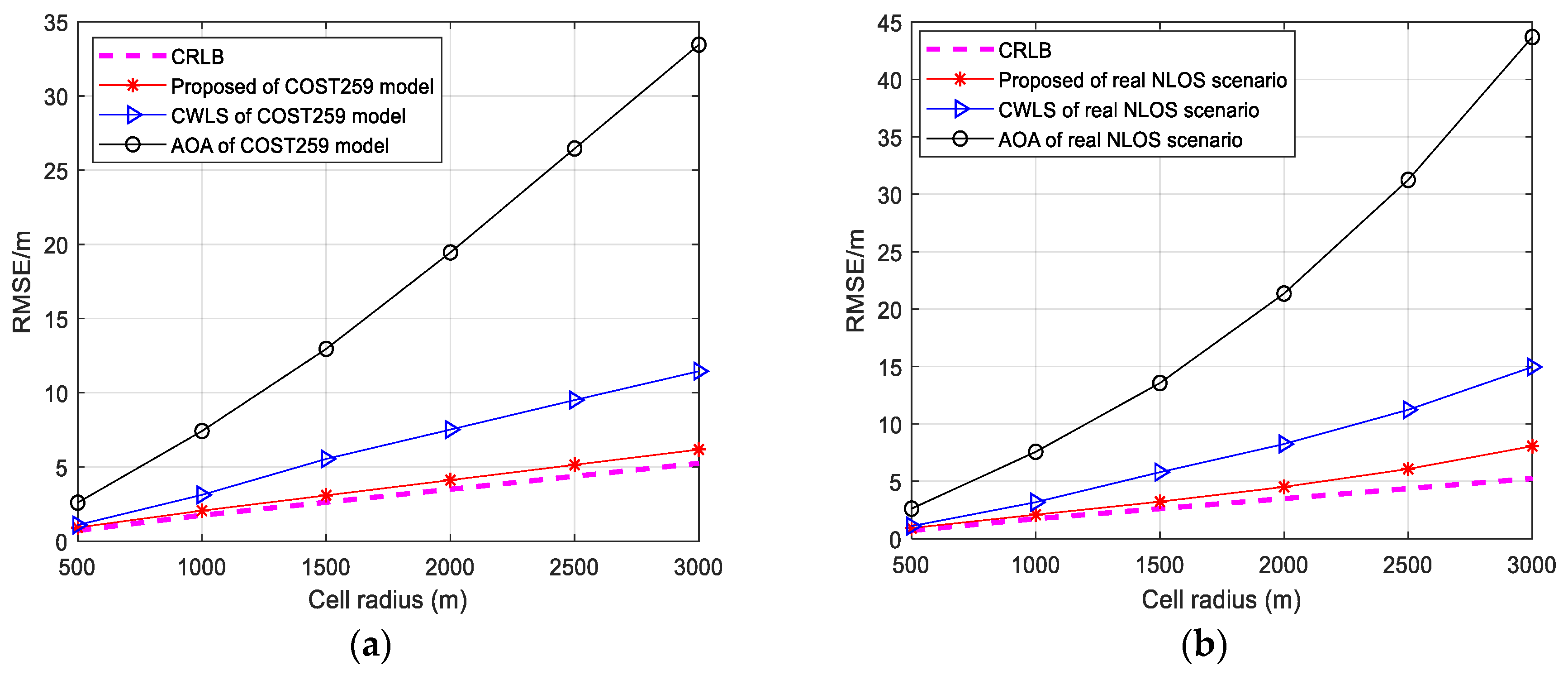
Figure 10 shows the performance with different number of service base stations, and the performance of actual NLOS scenario is worse than the performance of COST259 model. With increasing number of service base stations, the root-mean-square error (RMSE) location gradually decreases. The AOA method is considerably influenced by the number of base stations because of the NLOS error. The CWLS method has a lower RMSE; however, both of them perform poorly when the number of service base stations is less than four. The method proposed in this paper produces the most accurate performance because the PPO model can constantly correct the AOA measurements and reduce the influence of NLOS and measurement error.

3.2.3. Cell Radius

Figure 11 depicts the performance of different methods when the cell radii range from 500 m to 3000 m, and the performance of actual NLOS scenario is worse than the performance of COST259 model.

Figure 11 shows that with the increasing of cell radius, the RMSE location is increasing gradually, this is because large cell always has a large NLOS. When the cell radius is only 1000 m, these five methods have a similar performance, especially the methods of CWLS and the proposed one. When the cell radius is larger than 2000 m, the differences begin to grow, the methods of AOA has a bad performance, because these three algorithm are location through the AOA data directly. Compared with these three methods, the CWLS has a lower RMSE. The proposed method in this paper can obtain the best performance, this is because the PPO model can reduce the influence of NLOS and measurement error.

3.2.4. Channel Environment

Figure 12 depicts the performance of different channel environments, such as the additive white Gaussian noise (AWGN) channel and Rayleigh multi-path channel.

In the AWGN channel, both of the proposed algorithm and the CWLS method produce good location results. In a Rayleigh multi-path channel, because of the additional multi-path influence, the location RMSE increases. However, the proposed method also produces the best performance because the PPO can eliminate the multipath influence to some extent.

3.2.5. MS Velocity

Figure 13 depicts the performance of different methods with different MS speeds, and the performance of actual NLOS scenario is worse than the performance of COST259 model.

Figure 13 shows that with increasing of MS speed, the location RMSE gradually increases. The AOA methods are considerably influenced by MS speed; the trend is a geometric increase. The CWLS methods can reduce the location error of different MS speeds to a certain extent. The method proposed in this paper produces the best performance because the PPO model can reduce the influence of multiple paths.

4. Conclusions

To address the problem of AOA location, in this paper, we presented a new AOA passive location algorithm for an MIMO system based on PPO. This method uses PPO methods to correct the NLOS and measurement errors, and then determines the passive AOA location based on the least squares method. The experimental results showed that the proposed algorithm can determine the AOA location high accuracy. With the increasing of training data lengths and the number of base station, the RMSE of the proposed methods can be lower than 3 m. On the other hand, the RMSE of the proposed methods is almost less than 10 m at different MS velocity. PPO uses the ability of approximate arbitrary non-linear mapping and the fast learning property of deep reinforcement learning to effectively overcome the shortcomings of the traditional methods, such as AOA. In the future, we will apply the localization algorithm based on PPO to more complex sensor networks and channel environments.

References

1. Gazzah, L.; Najjar, L. Enhanced cooperative group localization with identification of LOS/NLOS BSs in 5G dense networks. Ad Hoc Netw. 2019, 89, 88–96. [Google Scholar] [CrossRef]
2. Joshi, J.; Grover, N.; Medikonda, P.; Gujral, V. Smart Wireless Communication System for Traffic Management and Localization. In Proceedings of the 6th Glob. Wirel. Summit, GWS 2018, Chiang Rai, Thailand, 25–28 November 2018; pp. 1–5. [Google Scholar]
3. Yassin, A.; Nasser, Y.; Awad, M.; Al-Dubai, A.; Liu, R.; Yuen, C.; Raulefs, R.; Aboutanios, E. Recent Advances in Indoor Localization: A Survey on Theoretical Approaches and Applications. IEEE Commun. Surv. Tutor. 2017, 19, 1327–1346. [Google Scholar] [CrossRef] [Green Version]
4. Sayed, A.H.; Tarighat, A.; Khajehnouri, N. Network-based wireless location: Challenges faced in developing techniques for accurate wireless location information. IEEE Signal Process. Mag. 2005, 22, 24–40. [Google Scholar] [CrossRef]
5. Güvenç, I.; Chong, C.C. A survey on TOA based wireless localization and NLOS mitigation techniques. IEEE Commun. Surv. Tutor. 2009, 11, 107–124. [Google Scholar] [CrossRef]
6. Doğançay, K.; Hmam, H. Optimal angular sensor separation for AOA localization. Signal Process. 2008, 88, 1248–1260. [Google Scholar] [CrossRef]
7. Shen, J.; Molisch, A.F.; Salmi, J. Accurate Passive Location Estimation Using TOA Measurements. IEEE Trans. Wirel. Commun. 2012, 11, 2182–2192. [Google Scholar] [CrossRef]
8. Dersan, A.; Tanik, Y. Passive radar localization by time difference of arrival. In Proceedings of the IEEE Military Communications Conference MILCOM, IEEE, Anaheim, CA, USA, 7–10 October 2002; Volume 2, pp. 1251–1257. [Google Scholar]
9. Echigo, H.; Ohtsuki, T.; Jiang, W.; Takatori, Y. Fair pilot assignment based on AOA and pathloss with location information in massive MIMO. In Proceedings of the GLOBECOM 2017 IEEE Global Communications Conference, Singapore, 4–8 December 2017; pp. 1–6. [Google Scholar]
10. Tang, H.; Park, Y.; Qiu, T. A TOA-AOA-based NLOS error mitigation method for location estimation. EURASIP J. Adv. Signal Process. 2007, 2008, 682528. [Google Scholar] [CrossRef] [Green Version]
11. Zhang, V.Y.; Wong, A.K.S. Combined AOA and TOA NLOS localization with nonlinear programming in severe multipath environments. In Proceedings of the 2009 IEEE Wireless Communications and Networking Conference, Budapest, Hungary, 5–8 April 2009; pp. 1–6. [Google Scholar]
12. Wang, F.; Liu, X. Empirical Analysis of TOA and AOA in Hybrid Location Positioning Techniques. IOP Conf. Ser. 2018, 466, 012089. [Google Scholar] [CrossRef] [Green Version]
13. Bianchi, V.; Ciampolini, P.; De Munari, I. RSSI-Based Indoor Localization and Identification for ZigBee Wireless Sensor Networks in Smart Homes. IEEE Trans. Instrum. Meas. 2019, 68, 566–575. [Google Scholar] [CrossRef]
14. Hua, J.; Yin, Y.; Lu, W.; Zhang, Y.; Li, F. NLOS identification and positioning algorithm based on localization residual in wireless sensor networks. Sensors 2018, 18, 2991. [Google Scholar] [CrossRef] [Green Version]
15. Koledoye, M.A.; Facchinetti, T.; Almeida, L. Mitigating effects of NLOS propagation in MDS-based localization with anchors. In Proceedings of the 2018 IEEE International Conference on Autonomous Robot Systems and Competitions (ICARSC), Torres Vedras, Portugal, 25–27 April 2018; pp. 148–153. [Google Scholar]
16. Shikur, B.Y.; Weber, T. Tdoa/aod/aoa localization in nlos environments. In Proceedings of the 2014 IEEE International Conference on Acoustics, Speech and Signal Processing (ICASSP), Florence, Italy, 4–9 May 2014; pp. 6518–6522. [Google Scholar]
17. Li, Y.-Y.; Qi, G.-Q.; Sheng, A.-D. Performance metric on the best achievable accuracy for hybrid TOA/AOA target localization. IEEE Commun. Lett. 2018, 22, 1474–1477. [Google Scholar] [CrossRef]
18. Zhang, Y.; Yanbiao, X.I.; Gangwei, L.I.; Zhao, K. TDOA/AOA hybrid positioning algorithm based on Kalman filter in NLOS environment. Comput. Eng. Appl. 2015, 2015, 13. [Google Scholar]
19. Tian, X.; Yin, J. Position Location Estimation Algorithms for Mobile Station in NLOS Propagation Environment. In Proceedings of the 2018 Joint International Advanced Engineering and Technology Research Conference (JIAET 2018), Xi’an, China, 26–27 May 2018; Atlantis Press: Paris, France, 2018; Volume 137, pp. 272–277. [Google Scholar]
20. Hua, J.; Yin, Y.; Wang, A.; Zhang, Y.; Lu, W. Geometry-based non-line-of-sight error mitigation and localization in wireless communications. Sci. China Inf. Sci. 2019, 62, 1–15. [Google Scholar] [CrossRef] [Green Version]
21. Wang, Y.; Hang, J.; Cheng, L.; Li, C.; Song, X. A hierarchical voting based mixed filter localization method for wireless sensor network in mixed LOS/NLOS environments. Sensors 2018, 18, 2348. [Google Scholar] [CrossRef] [Green Version]
22. Cheng, C.; Hu, W.; Tay, W.P. Localization of a moving non-cooperative RF target in NLOS environment using RSS and AOA measurements. In Proceedings of the 2015 IEEE International Conference on Acoustics, Speech and Signal Processing (ICASSP), Brisbane, QLD, Australia, 19–24 April 2015; pp. 3581–3585. [Google Scholar]
23. Yu, H.; Huang, G.; Gao, J.; Liu, B. An efficient constrained weighted least squares algorithm for moving source location using TDOA and FDOA measurements. IEEE Trans. Wirel. Commun. 2011, 11, 44–47. [Google Scholar] [CrossRef]
24. Wang, X.; Wang, X.; Mao, S. CiFi: Deep convolutional neural networks for indoor localization with 5 GHz Wi-Fi. In Proceedings of the 2017 IEEE International Conference on Communications (ICC), Paris, France, 21–25 May 2017. [Google Scholar]
25. Wu, G.S.; Tseng, P.H. A Deep Neural Network-Based Indoor Positioning Method using Channel State Information. In Proceedings of the 2018 International Conference on Computing, Networking and Communications (ICNC), Maui, HI, USA, 5–8 March 2018; pp. 290–294. [Google Scholar]
26. Schulman, J.; Levine, S.; Abbeel, P.; Jordan, M.; Moritz, P. Trust region policy optimization. In Proceedings of the International Conference on Machine Learning, Lille, France, 6–11 July 2015; pp. 1889–1897. [Google Scholar]
27. Schulman, J.; Wolski, F.; Dhariwal, P.; Radford, A.; Klimov, O. Proximal policy optimization algorithms. arXiv 2017, arXiv:1707.06347. [Google Scholar]
28. Lillicrap, T.P.; Hunt, J.J.; Pritzel, A.; Heess, N.; Erez, T.; Tassa, Y.; Silver, D.; Wierstra, D. Continuous control with deep reinforcement learning. arXiv 2015, arXiv:1509.02971. [Google Scholar]
29. Hämäläinen, P.; Babadi, A.; Ma, X.; Lehtinen, J. PPO-CMA: Proximal Policy Optimization with Covariance Matrix Adaptation. arXiv 2018, arXiv:1810.02541. [Google Scholar]
30. Chen, G.; Peng, Y.; Zhang, M. An Adaptive Clipping Approach for Proximal Policy Optimization. arXiv 2018, arXiv:1804.06461. [Google Scholar]
31. Lee, K.; Oh, J.; You, K. TDOA/AOA based geolocation using Newton method under NLOS environment. In Proceedings of the 2016 IEEE International Conference on Cloud Computing and Big Data Analysis (ICCCBDA), ChengDu, China, 5–7 July 2016; pp. 373–377. [Google Scholar]
32. Aghaie, N.; Tinati, M.A. Localization of WSN nodes based on NLOS identification using AOAs statistical information. In Proceedings of the 2016 24th Iranian Conference on Electrical Engineering (ICEE), Shiraz, Iran, 10–12 May 2016; pp. 496–501. [Google Scholar]
33. Yu, K.; Bengtsson, M.; Ottersten, B.; McNamara, D.; Karlsson, P.; Beach, M. A wideband statistical model for NLOS indoor MIMO channels. In Proceedings of the Vehicular Technology Conference, IEEE 55th Vehicular Technology Conference, VTC Spring 2002 (Cat. No.02CH37367), Birmingham, AL, USA, 6–9 May 2002; pp. 370–374. [Google Scholar]
34. Aziz, M.A.; Allen, C.T. Experimental Results of a Differential Angle-of-Arrival Based 2D Localization Method Using Signals of Opportunity. Int. J. Navig. Obs. 2018, 2018. [Google Scholar] [CrossRef]
35. Cheung, K.W.; So, H.-C.; Ma, W.-K.; Chan, Y.-T. A constrained least squares approach to mobile positioning: Algorithms and optimality. EURASIP J. Adv. Signal Process. 2006, 2006, 20858. [Google Scholar] [CrossRef] [Green Version]
Figure 1. Diagram of proximal policy optimization (PPO) algorithm when A < 0.
Electronics 08 01558 g001
Figure 2. Diagram of PPO algorithm when A > 0.
Electronics 08 01558 g002
Figure 3. PPO training process.
Electronics 08 01558 g003
Figure 4. The actual non-line-of-sight (NLOS) measurement scenario: (a) distribution of base stations in the test environment; (b) the receiving antenna.
Electronics 08 01558 g004
Figure 5. Universal Software Radio Peripheral X310: (a) the front of X310; (b) the reverse side of X310.
Electronics 08 01558 g005
Figure 6. Process of the proposed algorithm.
Electronics 08 01558 g006
Figure 7. Average normalized rewards received during training.
Electronics 08 01558 g007
Figure 8. Corrected angle of arrival (AOA) data.
Electronics 08 01558 g008
Figure 9. The performance with different training data lengths.
Electronics 08 01558 g009
Figure 10. The accuracy of location with different training data length: (a) the performance of COST259 model; (b) the performance of actual NLOS scenario.
Electronics 08 01558 g010
Figure 11. The accuracy of location with different cell radii: (a) the performance of COST259 model; (b) the performance of actual NLOS scenario.
Electronics 08 01558 g011
Figure 12. The accuracy of location with different channel. On the x axis, 1 is the proposed, 2 is the constrained weighted least squares (CWLS) method in this paper, 3 is the AOA method in this paper.
Electronics 08 01558 g012
Figure 13. The performance of different algorithms with different MS speeds: (a) the performance of COST259 model; (b) the performance of actual NLOS scenario.
Electronics 08 01558 g013