A Novel Structure for a Multi-Bernoulli Filter without a Cardinality Bias

Abstract

The original multi-target multi-Bernoulli (MeMBer) filter for multi-target tracking (MTT) is shown analytically to have a significant bias in its cardinality estimation. A novel cardinality balance multi-Bernoulli (CBMeMBer) filter reduces the cardinality bias by calculating the exact cardinality of the posterior probability generating functional (PGFl) without the second assumption of the original MeMBer filter. However, the CBMeMBer filter can only have a good performance under a high detection probability, and retains the first assumption of the MeMBer filter, which requires measurements that are well separated in the surveillance region. An improved MeMBer filter proposed by Baser et al. alleviates the cardinality bias by modifying the legacy tracks. Although the cardinality is balanced, the improved algorithm employs a low clutter density approximation. In this paper, we propose a novel structure for a multi-Bernoulli filter without a cardinality bias, termed as a novel multi-Bernoulli (N-MB) filter. We remove the approximations employed in the original MeMBer filter, and consequently, the N-MB filter performs well in a high clutter intensity and low signal-to-noise environment. Numerical simulations highlight the improved tracking performance of the proposed filter.

1. Introduction

Considering the multi-target tracking (MTT) environments, the unknown number of targets changes with time because of the presence of target deaths and births. Moreover, the ambiguities in track-to-measurement association, which involves the missed detection and clutters, increase the difficulty of the joint estimation of the target cardinality and target states [1,2,3]. Based on the finite set statistics (FISST) theory, Mahler proposed a rigorous formulation of random finite set (RFS)-type filters. The RFS-based algorithms model the targets and the measurements as RFSs [3]. Compared with the conventional multiple hypothesis tracker (MHT) and joint probability data association (JPDA) algorithms [4,5,6], they avoid data association, which has a high computation burden. In the past few years, several RFS-based methods, such as the well-known probability hypothesis density (PHD) filter [7,8,9], cardinality PHD (CPHD) filter [10,11,12], and MeMBer filter [3] have been created. For example, the PHD filter models both targets and measurements as Poisson RFSs, and sequentially propagates the first moment of the multi-target density (PHD intensity) over time. The CPHD filter improves the cardinality-estimating performance of the PHD filter by propagating the cardinality distribution with the PHD of the multi-target density. The MeMBer filter parameterizes the multi-target distribution that models each potential target as a single Bernoulli RFS [3], which is characterized by the probability of existence and the probability density function (pdf). Accordingly, the multi-Bernoulli (MB) RFS is a union of multiple independent Bernoulli components. Since the Gaussian mixture implementations are proposed for the RFS-based filters, various extensions are found in many papers [3,13]. However, some inherent problems brought about by the assumptions made in these filters limit their applications.

Recently, the conjugate distributions in the framework of Bayesian probability theory has generated substantial interest. A conjugate distribution means that the Bayesian recursion is closed. Those filters based on conjugate priors derived under the labeled RFS [14,15,16] and unlabeled RFS theory [17,18,19,20] can approximate the exact multi-target distributions accurately and were compared in Vo et al. [21]. The Poisson multi-Bernoulli mixture (PMBM) filter is derived based on the unlabeled distributions, where the filter models multi-target using a hybrid form of Poisson and MB mixture (MBM) RFSs. The prior multi-target distribution is the same with the posterior multi-target distribution in the PMBM filter [17,18]. Another Bayes-closed filter is derived based on the well-known generalized labeled multi-Bernoulli distribution (GLMB) [14,15,16], along with a relatively efficient version, the well-known δ-GLMB filter, which propagates the whole data association history together with track sets; consequently, it is computationally expensive. The LMB filter was proposed in Williams [16] based on approximating the GLMB density. However, the prediction step in the standard form of the δ-GLMB and the LMB filter involves truncating prediction density by a K-shortest path algorithm, which brings in additional computational burden and influences the efficiency of performance. Thus, combining the prediction and update step of these filters is necessary for practical application [22,23].

However, the RFS formulation using the FISST theory is free of the huge computational burden due to the data association in MTT [3,24]. Some approximations made in the MeMBer filter may bring in a significant performance degradation. For example, the MeMBer filter has a positive cardinality bias due to the approximations made in the derivation of the MeMBer corrector to obtain a posterior multi-Bernoulli density (second approximation). The CBMeMBer filter achieves the cardinality balance by preserving the PHD of each Bernoulli component [25]; however, this approximation has destroyed the posterior density, especially in low-detection (low signal-to-noise) environments. An improved form of the MeMBer (I-MeMBer) filter models the spurious targets in the legacy tracks and removes them after the update step [26]. Consequently, the cardinality is balanced. However, both CBMeMBer and I-MeMBer filters retain the first approximation of the MeMBer filter [3], which requires measurements that are well-separated in surveillance region. Thus, they cannot perform well in a surveillance region with proximity targets and/or high clutter density environments. The measurement-driven MeMBer filter removes the cardinality bias by modifying the legacy parameters, but it is not an analytical solution [27].

In this paper, an analytical solution to the Bayesian multi-target filter is proposed. The targets are modeled as an MB RFS, where each target is modeled as a Bernoulli RFS with an individual existence probability and pdf. The prior multi-Bernoulli distribution shifts the combinatorial problem to that of associating measurements to a corresponding Bernoulli component. Thus, the approximation employed in the original MeMBer filter is relaxed. The proposed novel structure of the multi-Bernoulli (N-MB) filter employs a Gibbs sampler [28] to solve the data association problem, i.e., it finds a finite number of best global hypothesis.

The remainder of this paper is organized as follows. In Section 2, we review the background information on RFS theory. In Section 3, we derive our N-MB filter. In Section 4, we present the implementation details for the N-MB filter. In Section 5, we show the performance of our proposed N-MB filter. Conclusions are given in Section 6.

2. Random Finite Set Statistics

The RFS is a finite-set-valued random variable, and throughout this paper, we model the multi-target as the union of a Poisson RFS and a MB RFS. An RFS includes a random number and unordered targets and represents individual states as random vectors. A finite set of state vectors $X$ is used to denote multi-target states, where $X=\left\{x_1,\dots ,x_n\right\}$. The cardinality of a finite set is $\left|X\right|$. Denote the probability density of the RFS with $\pi \left(X\right)$ and the set of all finite subsets of the state space $\mathbb{X}$ with $\mathcal{F}\left(\mathbb{X}\right)$, then for a function $f:\mathcal{F}\left(\mathbb{X}\right)\to \mathbb{R}$, the set integral is given as:

$${\displaystyle \int f\left(X\right)}\delta X={\displaystyle \sum _{i=0}^{\infty }\frac{1}{i!}{\displaystyle {\int }_{{\mathbb{X}}^i}f\left(\left\{x_1,\dots ,x_i\right\}\right)d\left(x_1,\dots ,x_i\right)}}$$

(1)

Defining a multi-target exponential notation $h^X\triangleq {\displaystyle \prod _{x\in X}h\left(x\right)}$, where $h$ is a real-valued function with $h^{Ø}=1$. The PGFl is given as:

$$G\left[h\right]={\displaystyle \int h^X\pi \left(X\right)\delta X}.$$

(2)

A Bernoulli RFS with an existence probability $r$ and pdf $p(\cdot )$ has a multi-target density and PGFl:

$$f\left(X\right)=\{\begin{array}{ll}1-r,\hfill & X=Ø\\ r\cdot p\left(x\right),\hfill & X=\left\{x_i\right\}\\ 0,\hfill & \mathrm{otherwise}\end{array},$$

(3)

$$G\left[h\right]=1-r+r\cdot \langle p,h\rangle ,$$

(4)

where $\langle a,b\rangle \triangleq {\displaystyle \int a\left(x\right)b\left(x\right)dx}$ denotes the inner product of two functions $a(\cdot )$ and $b(\cdot )$. An MB density is the union of multiple independent Bernoulli densities:

$$\pi \left(\left\{X_1,\dots ,X_n\right\}\right)=\pi (Ø){\displaystyle \sum _{1\le i_1\ne \cdots \ne i_n\le N}{\displaystyle \prod _{j=1}^n\frac{r_{i_j}{p}_{i_j}\left(X_j\right)}{1-r_{i_j}}}},$$

(5)

where $N$ is the number of single Bernoulli components in an MB and $\pi (Ø)={\displaystyle {\prod }_{j=1}^N\left(1-r_j\right)}$. Furthermore, its PGFl is given as:

$$G_Y\left[h\right]={\displaystyle \prod _{i=1}^N\left(1-r^{\left(i\right)}+r^{\left(i\right)}\langle p^{\left(i\right)},h\rangle \right)},$$

(6)

Throughout this paper, an MB distribution is abbreviated as:

$$\pi \left(X\right)={\left\{\left(r_j,p_j\right)\right\}}_{j=1}^N.$$

(7)

Given a Dirac delta density ${\delta }_x$, we define the functional derivative of $F\left[h\right]$ in the direction of ${\delta }_x$ as $\frac{\delta F}{\delta x}\left[h\right]\triangleq \frac{\partial F}{\partial {\delta }_x}\left[h\right]$ and given as:

$$\frac{\delta F}{\delta x}\left[h\right]=\underset{\epsilon \searrow 0}{\lim }\frac{F\left[h+\epsilon {\delta }_x\right]-F\left[h\right]}{\epsilon }.$$

(8)

If the functional $F\left[h\right]$ is of the form $F\left[h\right]={\displaystyle \int h\left(x\right)g\left(x\right)dx}$, then we have $\frac{\delta F}{\delta x}\left[h\right]=g\left(x\right)$.

The first-order moment, i.e., the PHD function $D(\cdot )$ of a multi-target density $\pi (\cdot )$, is given as:

$$D\left(x\right)={\frac{\delta G}{\delta x}\left[h\right]|}_{h\left(x\right)=1,\forall x}.$$

(9)

The PHD function of an MB is given as [3]:

$$D^{MB}\left(x\right)={\displaystyle \sum _{i=1}^N{r}^{\left(i\right)}\cdot p^{\left(i\right)}\left(x\right)}.$$

(10)

A key result of the functional derivative utilized in our derivation process is the product rule [3]:

$$\frac{\delta F}{\delta Z}\left(F_0\left[h\right]\dots F_n\left[h\right]\right)={\displaystyle \sum _{W_0\uplus \dots \uplus W_n=Z}\frac{\delta F_0}{\delta W_0}\left[h\right]\dots }\frac{\delta F_n}{\delta W_n}\left[h\right],$$

(11)

where $\uplus$ indicates the sum is over all disjoint sets $W_0,\dots ,W_n$ and $W_0,\cup \dots \cup W_n=Z$, which permits the calculation of the derivative of a product of an MB PGFl.

3. Novel Structure of an MB Filter

In this section, the derivation process of the proposed algorithm is presented. Before we commence, the following assumptions are presented, which are used in the derivation of the algorithm.

Assumptions:

• Birth target distribution is denoted by ${\pi }_k^b={\left\{\left(r_{b,k}^{\left(i\right)},p_{b,k}^{\left(i\right)}\right)\right\}}_i^{N_k^b}$.
• The survival probability conditioned on the target state is $p_S\left(x\right)$. The transition pdf is $f_{k|k-1}\left(x|\zeta \right)$, where $\zeta$ denotes the previous target state.
• The clutter distribution is modeled as a Poisson distribution with a clutter rate ${\lambda }_C$.
• A single target may generate at most one measurement, where the detection probability is $p_D\left(x\right)$ and the measurement likelihood is $g\left(z|x\right)$.

3.1. Derivation of the Predictor

At each time $k-1$, the PGFl $G_{k-1|k-1}\left[h\right]$ of the posterior MB density and the PGFl $G_k^b\left[h\right]$ of the birth density take the form of Equation (6). The predicted multi-target distribution $f_{k|k-1}\left(X|Z^{k-1}\right)$ is also a multi-target multi-Bernoulli process [3]:

$$G_{k|k-1}\left[h\right]=G_k^b\left[h\right]\cdot {\displaystyle \prod _{i=1}^{N_{k|k-1}^p}\left(1-r_{p,k|k-1}^{\left(i\right)}+r_{p,k|k-1}^{\left(i\right)}\cdot \langle p_{p,k|k-1}^{\left(i\right)},h\rangle \right)}.$$

(12)

Here, $G_k^b\left[h\right]$ is the PGFl of the birth process, which follows Assumption 1:

$$G_k^b\left[h\right]={\displaystyle \prod _{i=1}^{N_k^b}\left(1-r_{b,k}^{\left(i\right)}+r_{b,k}^{\left(i\right)}\cdot \langle p_{b,k}^{\left(i\right)},h\rangle \right)}.$$

(13)

Also, the predicted parameters of the surviving targets are given as:

$$r_{p,k|k-1}^{\left(i\right)}=r_{p,k-1|k-1}^{\left(i\right)}\cdot \langle p_S,p_{p,k-1|k-1}^{\left(i\right)}\rangle ,$$

(14)

$$p_{p,k|k-1}^{\left(i\right)}\left(x\right)=\langle p_{S}f\left(x|\cdot \right),p_{p,k-1|k-1}^{\left(i\right)}\rangle .$$

(15)

3.2. Derivation of the Corrector

For notational simplicity, in the following derivation, we omit the time index. As given in the above subsection, the PGFl of the predicted distribution is the MB process:

$$G_{k|k-1}\left[h\right]={\displaystyle \prod _{i=1}^{N_{k|k-1}}\left(1-r_{k|k-1}^{\left(i\right)}+r_{k|k-1}^{\left(i\right)}\cdot \langle p_{k|k-1}^{\left(i\right)},h\rangle \right)},$$

(16)

where $N_{k|k-1}=N_k^b+N_{k|k-1}^p$.

Denoting the multi-target measurement likelihood function conditioned on the target state set $X$ as $L_k\left(Z|X\right)$, the PGFl of the likelihood $L_k\left(Z|X\right)$ is:

$$G\left[g|X\right]={\displaystyle \int g^Z{L}_k\left(Z|X\right)\delta Z}=\exp \left\{\langle v^{fa},g-1\rangle \right\}{\displaystyle \prod _{x\in X}\left\{1-p_D\left(x\right)+p_D\left(x\right)p_g\left(x\right)\right\}}$$

(17)

where $p_g\left(x\right)\triangleq {\displaystyle \int g\left(z\right)l_k\left(z|x\right)dz}$. Thus, the functional $F\left[g,h\right]$ is defined as:

$$\begin{array}{ll}F\left[g,h\right]& ={\displaystyle \int h^{X}G\left[g|X\right]{\pi }_{k|k-1}\left(X\right)\delta X}\\ & =\exp \left\{\langle v^{fa},g-1\rangle \right\}{\displaystyle \int {\left\{h\left(1-p_D+p_D{p}_g\right)\right\}}^X{f}_{k|k-1}\left(X\right)\delta X}\\ & =\exp \left\{\langle v^{fa},g-1\rangle \right\}{G}_{k|k-1}\left[h\left(1-p_D+p_D{p}_g\right)\right]\end{array}$$

(18)

The PGFl of the updated density ${\pi }_{k|k}\left(X\right)$ (updated by $Z_k$) is given as [3]:

$$G_{k|k}\left[h\right]=\frac{\frac{\delta F}{\delta Z_k}\left[0,h\right]}{\frac{\delta F}{\delta Z_k}\left[0,1\right]}\propto \frac{\delta F}{\delta Z_k}\left[0,h\right],$$

(19)

where $\frac{\delta F}{\delta Z_k}\left[0,h\right]$ is the functional derivative of $F$ in $g=0$ WRT the set $Z_k$.

Using the product rule given in Equation (11), we rewrite Equation (19) as:

$$\frac{\delta F}{\delta Z_k}\left[0,h\right]={\displaystyle \sum _{W_0\uplus \dots \uplus W_n=Z_k}\frac{\delta F_0}{\delta W_0}\left[0,h\right]\dots }\frac{\delta F_n}{\delta W_n}\left[0,h\right],$$

(20)

where

$$F_0\left[g,h\right]=\exp \left\{\langle v^{fa},g-1\rangle \right\}$$

(21)

$$F_i\left[g,h\right]=G_{k|k-1}^{\left(i\right)}\left[h\cdot \left(1-p_D\left(x\right)+p_D\left(x\right)p_{g_i}\left(x\right)\right)\right]$$

(22)

where $n\ge i>0.$

The notation $W_0$ denotes the set of clutters, i.e., the measurements not associated with any targets. The set can have any cardinality $\left|W_0\right|$ (the number of clutter alarms) that meets the constraint $W_0\uplus W_1\uplus \dots \uplus W_n=Z_k$. For $n\ge i>0$, the set $W_i$ denotes the set of measurements associated with the corresponding target (represented by the Bernoulli component). The cardinality of the set is $\left|W_i\right|\le 1$, where $\left|W_i\right|=0$ means the target is not detected. The set $W_i$ is given as:

$$W_i=\{\begin{array}{ll}Ø,\hfill & {\sigma }_i=0\hfill \\ \left\{z_k^j\right\},\hfill & {\sigma }_i=j\hfill \end{array},$$

(23)

where ${\sigma }_i=0$ if the $i\mathrm{th}$ target is not detected, and ${\sigma }_i=j$ if the $i\mathrm{th}$ target is associated with measurement $z_k^j$. The number of measurements is $N^z$. Defining an $N-tuple$ $\theta =\left({\sigma }_{1:N}\right)\in {\left\{0:N^z\right\}}^N$ to denote a choice of a one-to-one mapping, i.e., there are no distinct $i>0$, $i^{\prime }>0$ with ${\sigma }_i={\sigma }_{i^{\prime }}>0$. The set of all assignment vectors $\theta$ is denoted as $\mathsf{\Theta }$.

The functional derivative of $F_0$ in $g=0$ WRT the set $W_0$ is given as:

$$\frac{\delta F_0}{\delta W_0}\left[0,h\right]=e^{-{\lambda }_C}{\left({\lambda }_C{V}^{-1}\right)}^{\left|W_0\right|},$$

(24)

where $V$ denotes the “volume” of the surveillance region. For $n\ge i>0$, the functional derivative of $F_i$ in $g$ WRT the set $W_i=\left\{z_{{\sigma }_i}\right\}$ is given as:

$$\frac{\delta F_i}{\delta W_i}\left[g,h\right]=\frac{\delta }{\delta z_{{\sigma }_i}}\left[1-r^{\left(i\right)}+r^{\left(i\right)}\langle p^{\left(i\right)},h\left(1-p_D+p_D{p}_g\right)\rangle \right].$$

(25)

Furthermore, set $g=0$:

$$\frac{\delta F_i}{\delta z_{{\sigma }_i}}\left[0,h\right]=\{\begin{array}{ll}{r}^{\left(i\right)}\langle p^{\left(i\right)},h{p}_{D}l\left(z_{{\sigma }_i}|\cdot \right)\rangle ,& {\sigma }_i>0\\ 1-r^{\left(i\right)}+r^{\left(i\right)}\langle p^{\left(i\right)},h\left(1-p_D\right)\rangle ,& {\sigma }_i=0\end{array}.$$

(26)

Using the association notations and the results of Equations (24) and (26), we rewrite Equation (20) as:

$$\frac{\delta F}{\delta Z_k}\left[0,h\right]=e^{-\lambda }{\displaystyle \sum _{\theta \in \mathsf{\Theta }}{\displaystyle \prod _{j:\nexists {\sigma }_i=j}{\lambda }_C}}\times {\displaystyle \prod _{i:{\sigma }_i=0}\left(1-r^{\left(i\right)}+r^{\left(i\right)}\langle p^{\left(i\right)},h\left(1-p_D\right)\rangle \right)}\times {\displaystyle \prod _{i:{\sigma }_i>0}{r}^{\left(i\right)}\langle p^{\left(i\right)},h{p}_{D}l\left(z_{{\sigma }_i}|\cdot \right)\rangle }.$$

(27)

Note that the PGFl with the same form as Equation (27) is not an MB PGFl because of the additional sum according to different associations $\theta$. A multi-Bernoulli PGFl is shown in Equation (13), which is the product of single Bernoulli PGFls.

The original MeMBer filter [3] approximates the derivative of $F\left[g,h\right]$ in $g$ WRT the whole measurement set $Z_k$. Moreover, in the derivation of the corrector for the original MeMBer filter, the CBMeMBer filter, and the I-MeMBer filter, the approximation that there is no more than one measurement near a true target is indispensable; a performance degradation occurs when targets in the surveillance region are too close, or the clutter intensity is very high. In contrast, the form as given in Equation (27) is exact. However, the combinatorial problem in this formulation is tractable. Thus, we utilize a Gibbs sampler to find the best associations $\theta$.

3.3. PHD Intensity of the Posterior

Moreover, we approximate the posterior density with an MB distribution by calculating the PHD intensity (first-order moment). Thus, an MB RFS ${\overline{\pi }}_{k|k}(\cdot )$ is constructed with an identical PHD intensity to the truncated distribution ${\pi }_{k|k}(\cdot )$ (truncated with a finite number of best association $\theta$).

The PHD of the updated posterior is:

$$D_{k|k}\left(x\right)={\frac{\delta G_{k|k}\left[h\right]}{\delta x}|}_{h=1}={\frac{\frac{{\delta }^{2}F}{\delta x\delta Z_k}\left[0,h\right]}{\frac{\delta F}{\delta Z_k}\left[0,1\right]}|}_{h=1}.$$

(28)

We define the function:

$${\phi }_{\theta }\left[1\right]={\displaystyle \prod _{j:\nexists {\sigma }_i=j}{\lambda }_C{V}^{-1}}\times {\displaystyle \prod _{i:{\sigma }_i=0}\left(1-r^{\left(i\right)}+r^{\left(i\right)}\langle p^{\left(i\right)},\left(1-p_D\right)\rangle \right)}\times {\displaystyle \prod _{i:{\sigma }_i>0}{r}^{\left(i\right)}\langle p^{\left(i\right)},p_{D}l\left(z_{{\sigma }_i}|\cdot \right)\rangle }.$$

(29)

The derivative of the functional $F\left[0,h\right]$ in $h=1$ WRT the target state and measurement set $Z_k$ is given as:

$${\frac{{\delta }^{2}F}{\delta x\delta Z_k}\left[0,h\right]|}_{h=1}=e^{-{\lambda }_C}{\displaystyle \sum _{\theta \in \mathsf{\Theta }}{\phi }_{\theta }\left[1\right]{\displaystyle \sum _{i=1}^N{\varphi }_{\theta }\left(i\right)}},$$

(30)

where

$${\varphi }_{\theta }\left(i\right)=\{\begin{array}{ll}\frac{r^{\left(i\right)}\left(1-p_D\right)p^{\left(i\right)}}{1-r^{\left(i\right)}+r^{\left(i\right)}\langle p^{\left(i\right)},\left(1-p_D\right)\rangle },\hfill & {\sigma }_i=0\\ \frac{p_D{p}^{\left(i\right)}l\left(z_k^j|\cdot \right)}{\langle p^{\left(i\right)},p_{D}l\left(z_k^j|\cdot \right)\rangle },\hfill & {\sigma }_i=j\end{array}.$$

(31)

Thus, we rewrite Equation (28) as:

$$D_{k|k}\left(x\right)=\frac{{\displaystyle \sum _{\theta \in \mathsf{\Theta }}{\phi }_{\theta }\left[1\right]{\displaystyle \sum _{i=1}^N{\varphi }_{\theta }\left(i\right)}}}{{\displaystyle \sum _{\theta \in \mathsf{\Theta }}{\phi }_{\theta }\left[1\right]}}.$$

(32)

Equation (32) shows that the PHD function of the updated posterior has a similar structure to that of an MB PHD function, which is given in Equation (10). Thus, the Bernoulli components of ${\overline{\pi }}_{k|k}(\cdot )$ can be calculated from Equation (32) by merging the parameters of the $i\mathrm{th}$ Bernoulli component under different data associations $\theta$. The final MB parameters of ${\overline{\pi }}_{k|k}(\cdot )$ are given as:

$${\left\{\left({\overline{r}}_{k|k}^{\left(i\right)},{\overline{p}}_{k|k}^{\left(i\right)}(\cdot )\right)\right\}}_{i=1}^N={\displaystyle \underset{\theta \in \mathsf{\Theta }}{\cup }{\left\{\left(r_{\theta }^{\left(i\right)},p_{\theta }^{\left(i\right)}(\cdot )\right)\right\}}_{i=1}^N},$$

(33)

where

$$r_{\theta }^{\left(i\right)}=\{\begin{array}{ll}\frac{{\phi }_{\theta }\left[1\right]}{{\displaystyle \sum _{\theta \in \mathsf{\Theta }}{\phi }_{\theta }\left[1\right]}},\hfill & {\sigma }_i=j\\ \frac{{\phi }_{\theta }\left[1\right]}{{\displaystyle \sum _{\theta \in \mathsf{\Theta }}{\phi }_{\theta }\left[1\right]}}\times \frac{r^{\left(i\right)}\left(1-p_D\right)}{1-r^{\left(i\right)}+r^{\left(i\right)}\langle p^{\left(i\right)},\left(1-p_D\right)\rangle },\hfill & {\sigma }_i=0\end{array},$$

(34)

and

$$p_{\theta }^{\left(i\right)}=\{\begin{array}{ll}\frac{p_D{p}^{\left(i\right)}l\left(z_k^j|\cdot \right)}{\langle p^{\left(i\right)},p_{D}l\left(z_k^j|\cdot \right)\rangle },\hfill & {\sigma }_i=j\\ \frac{r^{\left(i\right)}\left(1-p_D\right)p^{\left(i\right)}}{\langle p^{\left(i\right)},\left(1-p_D\right)\rangle },\hfill & {\sigma }_i=0\end{array}.$$

(35)

From the right-hand side of Equation (33), we can see that there are many choices for the updated Bernoulli RFSs, but we can merge all the choices of associations for the Bernoulli components.

Compared to the LMB filter, our N-MB filter employs a straightforward prediction step. Thus, a different cost matrix needs to be designed to find the best data association. Moreover, the derivation of the LMB filter was based on approximating the GLMB density, which employs the labeled RFS notation. While our N-MB filter models the targets as an unlabeled multi-Bernoulli distribution, the Gibbs sampler is employed to get an approximate multi-Bernoulli distribution for the posterior density. Our N-MB filter was derived by using the theory of probability generating functionals and functional derivatives, which are very important tools for deriving RFS-based filters, for example, the PHD filter, CPHD filter, MeMBer filter, and PMBM filter.

4. Gaussian Implementation

In the previous section, we derived the recursion for the N-MB filter. Intuitively, the filter is intractable; therefore, approximations are necessary. In this section, we propose a closed-form Gaussian mixture (GM)-based implementation for the derived filter.

We assume that targets follow linear Gaussian dynamics, and measurements follow models with MB births:

$$f\left(x^i|x^{i-1}\right)=\mathcal{N}\left({\mathrm{x}}^i;F{x}^{i-1},Q\right),$$

(36)

$$g\left(z|x\right)=\mathcal{N}\left(z;Hx,R\right),$$

(37)

where $F$ denotes the transition matrix, $Q$ denotes the process noise covariance, $H$ denotes the observation matrix, and $R$ denotes the observation noise covariance. Furthermore, the survival and detection probability were assumed to be constant, which is given as $P_S\left(x\right)=P_S$ and $P_D\left(x\right)=P_D$.

The birth model is also an MB with the parameter set ${\left\{\left(r_{b,k}^{\left(i\right)},p_{b,k}^{\left(i\right)}(\cdot )\right)\right\}}_{i=1}^{N_k^b}$ and the pdf $p_{b,k}^{\left(i\right)}(\cdot )$ is a GM of the form:

$$p_{b,k}^{\left(i\right)}\left(x\right)={\displaystyle \sum _{l=1}^{J_{b,k}^{\left(i\right)}}{w}_{b,k}^{\left(i,l\right)}\mathcal{N}\left(x;m_{b,k}^{\left(i,l\right)},P_{b,k}^{\left(i,l\right)}\right),}$$

(38)

where $w_{b,k}^{\left(i,l\right)}$, $m_{b,k}^{\left(i,l\right)}$, and $P_{b,k}^{\left(i,l\right)}$ denote the weights, means, and covariances of the $l\mathrm{th}$ Gaussian component. Note that ${\displaystyle \sum _l{w}_{b,k}^{\left(i,l\right)}}=1$ and $j_{b,k}^{\left(i\right)}$ denotes the number of components.

4.1. Update

The prediction step of the proposed filter is the same with that in Baser et al. [25]. Given the predicted MB density ${\pi }_{k|k-1}={\left\{\left(r_{k|k-1}^{\left(i\right)},p_{k|k-1}^{\left(i\right)}\right)\right\}}_{i=1}^{N_{k|k-1}}$ and each pdf $p_{k|k-1}^{\left(i\right)}$ is in the form of Gaussian mixtures:

$$p_{k|k-1}^{\left(i\right)}={\displaystyle \sum _{l=1}^{J_{k|k-1}^{\left(i\right)}}{w}_{k|k-1}^{\left(i,l\right)}\mathcal{N}\left(x;m_{k|k-1}^{\left(i,l\right)},P_{k|k-1}^{\left(i,l\right)}\right)}$$

(39)

then, for each association $\theta$, the updated posterior MB density is:

$${\pi }_{\theta ,k|k}={\left\{\left(r_{\theta ,k|k}^{\left(i\right)}\left(z_{{\sigma }_i}\right),p_{\theta ,k|k}^{\left(i\right)}\left(\cdot ;z_{{\sigma }_i}\right)\right)\right\}}_{i=1}^{N_{k|k-1}}.$$

(40)

For ${\sigma }_i=0$, the updated means and covariances of the posterior MB density stay unchanged. For ${\sigma }_i>0$, the means and covariances of the posterior MB density are updated by the associated measurement $\left\{z_{{\sigma }_i}\right\}$:

$$w_{{\sigma }_i,k}^{\left(i,l\right)}=w_{k|k-1}^{\left(i,l\right)}\mathcal{N}\left(z;H_k{m}_{k|k-1}^{\left(i,l\right)},H_k{P}_{k|k-1}^{\left(i,j\right)}{H}_k^T+R_k\right)$$

(41)

$$m_{{\sigma }_i,k}^{\left(i,l\right)}=m_{k|k-1}^{\left(i,l\right)}+K_k^{\left(i,l\right)}\left(z_{{\sigma }_i}-H_k{m}_{k|k-1}^{\left(i,l\right)}\right),$$

(42)

$$P_{{\sigma }_i,k}^{\left(i,l\right)}=\left[I-K_k^{\left(i,l\right)}{H}_k\right]P_{k|k-1}^{\left(i,l\right)},$$

(43)

$$K_k^{\left(i,l\right)}=P_{k|k-1}^{\left(i,l\right)}{H}_k^T{\left[H_k{P}_{k|k-1}^{\left(i,l\right)}{H}_k^T+R_k\right]}^{-1}.$$

(44)

Then, the updated parameters in Equation (40) can be calculated using:

$$r_{\theta }^{\left(i\right)}=\{\begin{array}{ll}\frac{{{\phi }^{\prime }}_{\theta }\left[1\right]}{{\displaystyle \sum _{\theta \in \mathsf{\Theta }}{{\phi }^{\prime }}_{\theta }\left[1\right]}},\hfill & {\sigma }_i>0\\ \frac{{{\phi }^{\prime }}_{\theta }\left[1\right]}{{\displaystyle \sum _{\theta \in \mathsf{\Theta }}{{\phi }^{\prime }}_{\theta }\left[1\right]}}\cdot \frac{r\left(1-p_D\right)}{1-r{p}_D},\hfill & {\sigma }_i=0\end{array},$$

(45)

$$p_{\theta }^{\left(i\right)}=\{\begin{array}{ll}\frac{{\displaystyle {\sum }_{l=1}^{J_{k|k-1}^{\left(i\right)}}{w}_{{\sigma }_i,k}^{\left(i,l\right)}\mathcal{N}\left(x;m_{{\sigma }_i,k}^{\left(i,l\right)},P_{{\sigma }_i,k}^{\left(i,l\right)}\right)}}{{\displaystyle {\sum }_{l=1}^{J_{k|k-1}^{\left(i\right)}}{w}_{{\sigma }_i,k}^{\left(i,l\right)}}},\hfill & {\sigma }_i>0\\ p_{k|k-1}^{\left(i\right)},\hfill & {\sigma }_i=0\end{array},$$

(46)

where

$${{\phi }^{\prime }}_{\theta }\left[1\right]={\displaystyle \prod _{i:{\sigma }_i=0}\left(1-r_{k|k-1}^{\left(i\right)}{p}_D\right)}\times {\displaystyle \prod _{i:{\sigma }_i>0}\frac{r_{k|k-1}^{\left(i\right)}{\displaystyle {\sum }_{l=1}^{J_{k|k-1}^{\left(i\right)}}{p}_D{w}_{k|k-1}^{\left(i,l\right)}\mathcal{N}\left(x;m_{{\sigma }_i,k}^{\left(i,l\right)},P_{{\sigma }_i,k}^{\left(i,l\right)}\right)}}{{\lambda }_C{V}^{-1}}}.$$

(47)

The derivation of the above steps involves analytically calculating the products of Gaussians and integrals of Gaussians using the standard results of Gaussian functions [9].

4.2. Gibbs Sampling

We employ the Gibbs sampling algorithm to solve the data association problem, which is an efficient algorithm for finding the best choices for the assignment of targets to measurements [28]. This subsection presents the implementation of the integrated Gibbs sampler in detail.

After the prediction step, there are $N$ predicted Bernoulli components (representing $N$ targets), and the number of measurements is $N^z$. We define:

$${\eta }_i\left(j\right)=\frac{r^{\left(i\right)}{\displaystyle \sum _{l=1}^{J^{\left(i\right)}}{w}^{\left(i,l\right)}\mathcal{N}\left(x;m_{{\sigma }_i,k}^{\left(i,l\right)},P_{{\sigma }_i,k}^{\left(i,l\right)}\right)}}{\left[1-r^{\left(i\right)}+r^{\left(i\right)}\left(1-p_D\right)\right]{\lambda }_C{V}^{-1}},$$

(48)

where ${\sigma }_i=j\in \left\{1:N^z\right\}$ denotes the index of whichever measurement is assigned to the $i\mathrm{th}$ target. For ${\sigma }_i=0$, ${\eta }_i\left(0\right)=1$.

Consider a realization of a random variable $\theta$ that distributes according to a probability distribution $\pi$ on ${\left\{0:N^z\right\}}^N$. A Gibbs sampler is used to generate positive one-to-one vectors by independently sampling from $\pi$. The distribution $\pi$ is:

$$\pi \left(\theta \right)\propto 1_{\mathsf{\Gamma }}\left(\theta \right){\displaystyle \prod _{i=1}^n{\eta }_i\left({\sigma }_i\right)},$$

(49)

where $\mathsf{\Gamma }$ is the set of one-to-one mapping vectors in ${\left\{0,N^z\right\}}^N$.

It is difficult to sample from the distribution in Equation (49) directly. The Markov chain Monte Carlo (MCMC) method is the well-known algorithm for sampling from a complex distribution [29]. The Gibbs sampling algorithm is an efficient case of the so-called Metropolis–Hasting MCMC algorithm [30]. The proposed samples in a Gibbs sampler are always adopted; therefore, the Gibbs sampler is considered to be an efficient tool for generating the best associations [22,28,30,31]. Given results obtained using Equation (48), the assignment problem can be immediately solved by utilizing a Gibbs sampler.

Finally, the pseudocode for the filter is summarized in Algorithm 1.

Algorithm 1: Pseudocode for the filter

1. Step 1: (prediction) 2. Input birth density ${\left\{\left(r_{b,k}^{\left(i\right)},p_{b,k}^{\left(i\right)}\right)\right\}}_{i=1}^{N_{b,k}}$ and posterior density ${\left\{\left(r_{k-1}^{\left(i\right)},p_{k-1}^{\left(i\right)}\right)\right\}}_{i=1}^{N_{k-1}}$ 3. Output ${\left\{\left(r_{k|k-1}^{\left(i\right)},p_{k|k-1}^{\left(i\right)}\right)\right\}}_{i=1}^{N_{k|k-1}}$ 4. Step 2: (find best $\theta$) 5.   Calculate $\eta$ according to Equation (48) 6.   ${\left\{\theta \right\}}_{\theta \in \mathsf{\Theta }}=\mathrm{unique}\left(\mathrm{Gibbs}\right({\theta }^1,T,\eta \left)\right)$ 7. Step 3: (update for each $\theta$) 8. for $\theta \in \mathsf{\Theta }$ 9.   Calculate $r_{\theta }^{\left(i\right)}$, $p_{\theta }^{\left(i\right)}$ according to Equations (45) and (46) 10. end 11. Step 4: (reconstruction) 12. Reconstruct the MB density according to Equation (33)

5. Simulation

This section demonstrates the simulation results of the proposed N-MB filter conducted on linear Gaussian models. We set the simulation environments similar those in Baser et al. [25]. Consider a 2-D cartesian coordinate system where targets’ births and deaths occurred in a surveillance region of $\left[-1000,1000\right]\times \left[-1000,1000\right]\mathrm{m}$. A sensor was located at $\left(0,0\right)\mathrm{m}$ and provided point measurements to a controller at each time step. The sample interval was $\Delta =1\mathrm{s}$ and both the number and states of the multi-target at each time step were unknown. 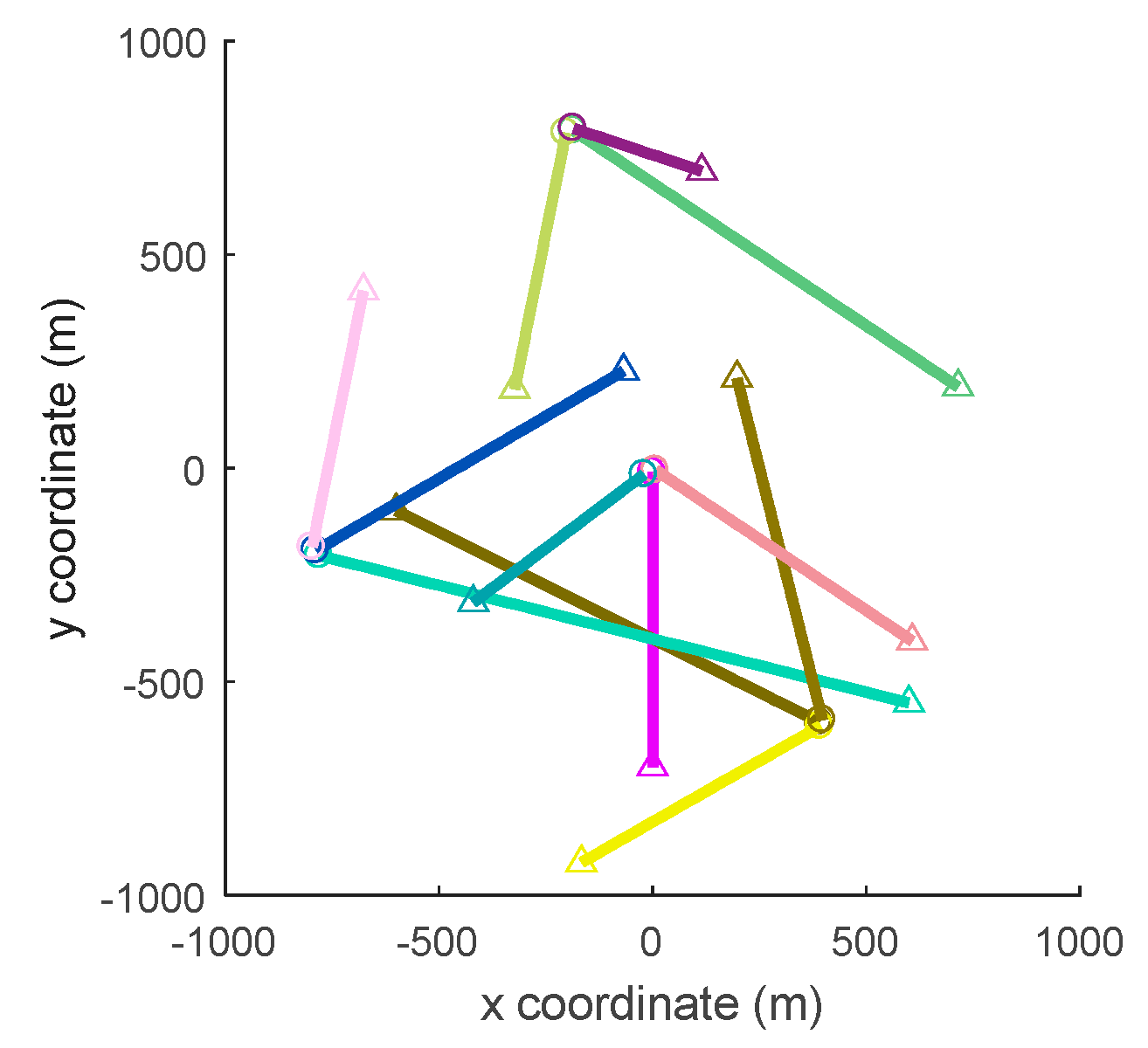Figure 1 shows the true tracks of targets.

5.1. Targets Model

The kinematic state is given as $\zeta ={\left[p_x,{\dot{p}}_x,p_y,{\dot{p}}_y\right]}^T$. The Gaussian target dynamics were modeled using the constant velocity (CV) model:

$$F_k^{\mathrm{CV}}=\left[\begin{array}{cccc}1& \Delta & 0& 0\\ 0& 1& 0& 0\\ 0& 0& 1& \Delta \\ 0& 0& 0& 1\end{array}\right],Q_k={\sigma }_v^2\left[\begin{array}{cccc}\frac{{\Delta }^4}{4}& \frac{{\Delta }^3}{2}& 0& 0\\ \frac{{\Delta }^3}{2}& {\Delta }^2& 0& 0\\ 0& 0& \frac{{\Delta }^4}{4}& \frac{{\Delta }^3}{2}\\ 0& 0& \frac{{\Delta }^3}{2}& {\Delta }^2\end{array}\right],$$

(50)

where the standard deviation (std) was set as ${\sigma }_v=5{\mathrm{m}/\mathrm{s}}^2$.

The survival probability was $p_S=0.98$ and the detection probability was set as a constant $p_D$. Consider the surveillance region including four locations where targets may birth from: $\left[0,0\right]\mathrm{m}$, $\left[400,-600\right]\mathrm{m}$, $\left[-800,-200\right]\mathrm{m}$, and $\left[-200,800\right]\mathrm{m}$. The birth process was modeled as a Poisson RFS with intensity $v^b\left(x\right)={\displaystyle {\sum }_{i=1}^4{w}_b\mathcal{N}\left(x;m_b^{\left(i\right)},P_b\right)}$, where $w_b=0.05$, $m_b^{\left(1\right)}={\left[0,0,0,0\right]}^T$, $m_b^{\left(2\right)}={\left[400,0,-600,0\right]}^T$, $m_b^{\left(3\right)}={\left[-800,0,-200,0\right]}^T$, and $m_b^{\left(4\right)}={\left[-200,0,800,0\right]}^T$, and the covariance matrix was given by $P_b=\mathrm{diag}{\left({\left[10,10,10,10\right]}^T\right)}^2$.

Measurements followed the observation function in Equation (37) with parameters:

$$H_k=\left[\begin{array}{llll}1\hfill & 0\hfill & 0\hfill & 0\hfill \\ 0\hfill & 0\hfill & 1\hfill & 0\hfill \end{array}\right],R_k={\sigma }_{\epsilon }^2\left[\begin{array}{cc}1& 0\\ 0& 1\end{array}\right],$$

(51)

where ${\sigma }_{\epsilon }=10\mathrm{m}$ was the std of the measurement noise. Clutters were modeled as a Poisson process with a clutter rate ${\lambda }_C$ and uniformly distributed according to the spatial probability density $1/V$ over the surveillance region, where $V=4\times {10}^6{\mathrm{m}}^2$ was the “volume” of the surveillance region.

We used a threshold $r_{\mathrm{TH}}=0.7$ for the target state extraction and we removed those Gaussian components whose weights were lower than ${10}^{-5}$. Those Gaussian components in a Bernoulli component whose distances were lower than $4\mathrm{m}$ were merged.

5.2. Performance Evaluation

Simulations were performed using MTT filters implemented in MATLAB (9.1.0.441655 R2016b, MathWorks, Beijing, China) on computers with an Intel Core i7-7700K CPU @ 4.20GHz and 16 GB RAM. We analyzed the performance in terms of the position estimates obtained by the proposed N-MB filer and CBMeMBer filter proposed in Baser et al. [25], the CPHD filter proposed in Vo et al. [13], and the track-oriented marginal MeMBer-Poisson (TOMB/P) filter proposed in García-Fernández et al. [17] using Monte Carlo simulations. We employed the optimal sub-pattern assignment (OSPA) distance as the error metric [32] to compare the performance of these filters. The OSPA is a distance metric for denoting the difference between two sets of points. The generalized OSPA (GOSPA), which was proposed recently, was also employed to verify the simulation’s performance. GOSPA penalizes localization errors for detected targets and the errors due to missed and false targets [33], which is not considered in OSPA. The GOSPA metric with parameter $\alpha =2$ is given by

$$\begin{array}{l}{d}_p^{\left(c,2\right)}\left(X,Y\right)\triangleq [\underset{\gamma \in {\mathsf{\Gamma }}^{\left(\left|X\right|,\left|Y\right|\right)}}{\min }({\displaystyle \sum _{\left(i,j\right)\in \gamma }d{\left(x_i,y_j\right)}^p}{+\frac{c^p}{2}\left(\left|X\right|+\left|Y\right|-2\left|\gamma \right|\right))]}^{\frac{1}{p}}\end{array}$$

(52)

where ${\mathsf{\Gamma }}^{\left(\left|X\right|,\left|Y\right|\right)}$ denotes the set of all possible assignments, $c$ is the cut-off value, and $p$ determines the severity of penalizing the outliers in the localization component. We compared the root mean square (RMS) OSPA and the RMS GOSPA for the position estimation across all time steps. The Euclidean metric was used as the base metric and we set $p=2$ and $c=300$. In this case, ${\left[d_p^{\left(c,2\right)}\left(\cdot ,\cdot \right)\right]}^2$ could be decomposed as: $c_l^2\left(\cdot ,\cdot \right)={\displaystyle \sum _{\left(i,j\right)\in \gamma }d{\left(x_i,y_j\right)}^p}$, which denotes the localization error; $c_m^2\left(\cdot ,\cdot \right)=c^p\left(\left|X\right|-\left|\gamma \right|\right)/2$, which denotes the miss-detection error; and $c_f^2\left(\cdot ,\cdot \right)=c^p\left(\left|Y\right|-\left|\gamma \right|\right)/2$, which denotes the false-detection error.

5.3. Simulation Results

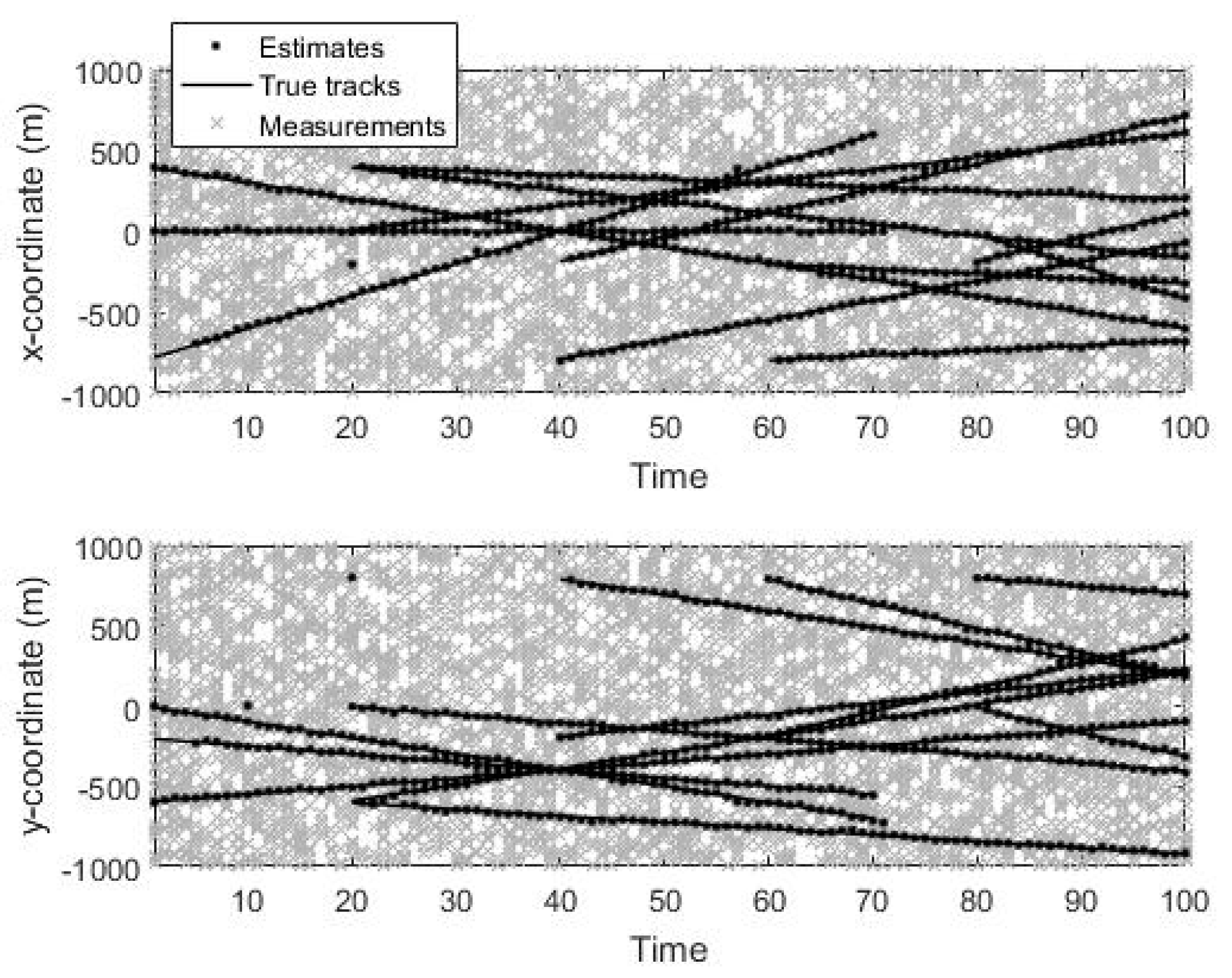
In Figure 2, the decomposed $x$- and $y$-components of the true tracks, state estimates generated by the N-MB filter, and measurements across all the time steps are shown versus time. The results showed that the proposed filter could correctly track the targets with individual motions throughout the targets’ births and deaths. Three targets crossed with each other at time step $k=40$, and two targets crossed with each other at time step $k=60$, and the proposed filter had no difficulty handling these situation.

We further showed the performance of our proposed N-MB filter over $N_{MC}=200$ Monte Carlo (MC) runs with a fixed set of target trajectories (shown in Figure 1) but randomly generated measurement data (the generated measurements over all time steps for one MC run is shown in Figure 2). 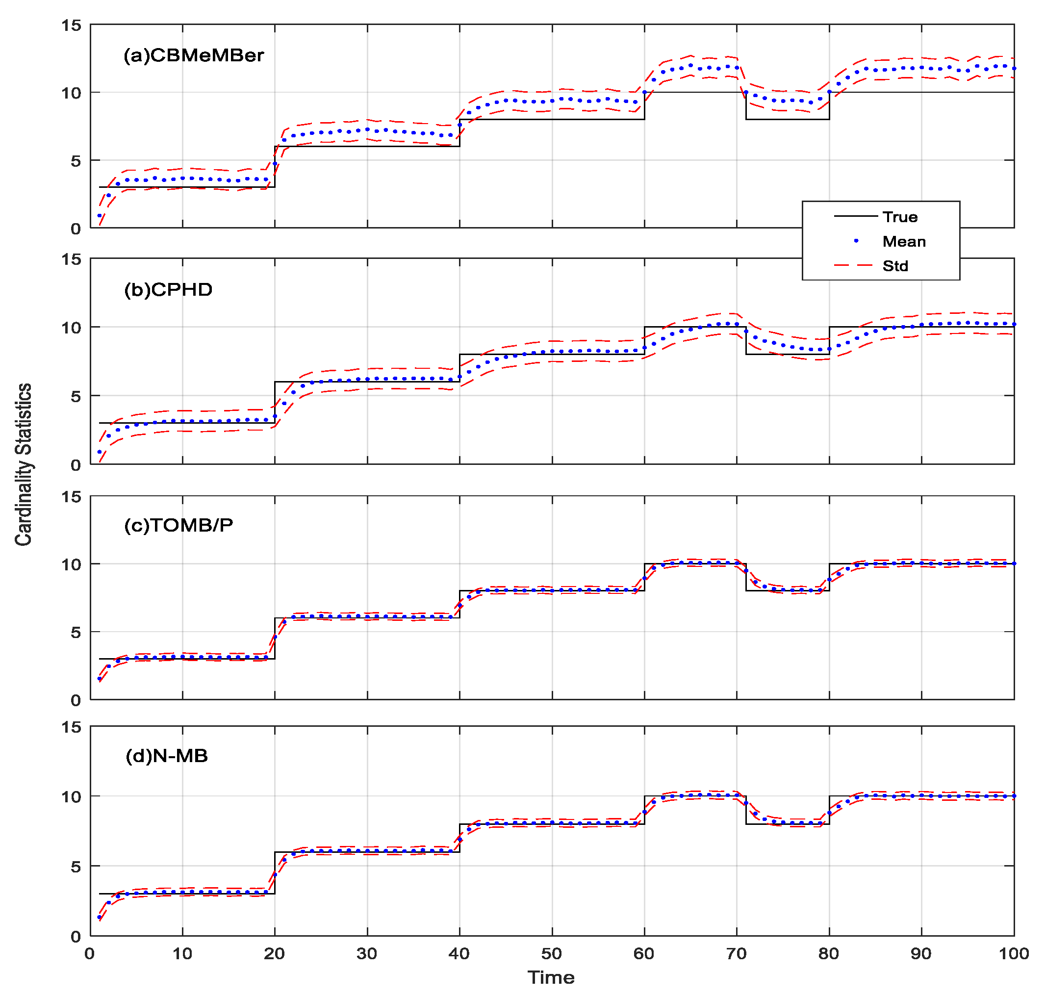Considering an environment with a high clutter intensity (the clutter rate was set to ${\lambda }_C=80$ and the detection probability was set as $p_D=0.98$), the mean and std of the estimated cardinality versus time for the CBMeMBer, CPHD, TOMB/P, and N-MB filters are shown in Figure 3. The CBMeMBer filter suffers from false estimations greatly. This phenomenon is easy to explain because the CBMeMBer employed the assumption that measurements were well separated [3,25]. In contrast, both TOMB/P and the proposed N-MB filter performed well in the cardinality estimation, and had a lower variance than the CPHD filter.

Moreover, the MC average of the RMS OSPA distances are given in Figure 4, where the clutter rate was set to ${\lambda }_C=20$ and the detection probability was set to $p_D=0.7$ (i.e., a low signal-to-noise environment). The CBMeMBer filter suffered a great performance degradation when the detection probability was low. This was because the filter required the approximation of a high detection probability to correct for the negative term involved in the existence probability of the resulting MB components [25,34]. In contrast, the proposed N-MB filter performed well in the environment with a low detection probability. Compared to the TOMB/P filter, the N-MB filter had a better performance in most of time steps, but the TOMB/P filter outperformed the N-MB filter in terms of removing death targets at $k=71$. The CPHD filter was also not suitable for application in the low-signal-to-noise environment.

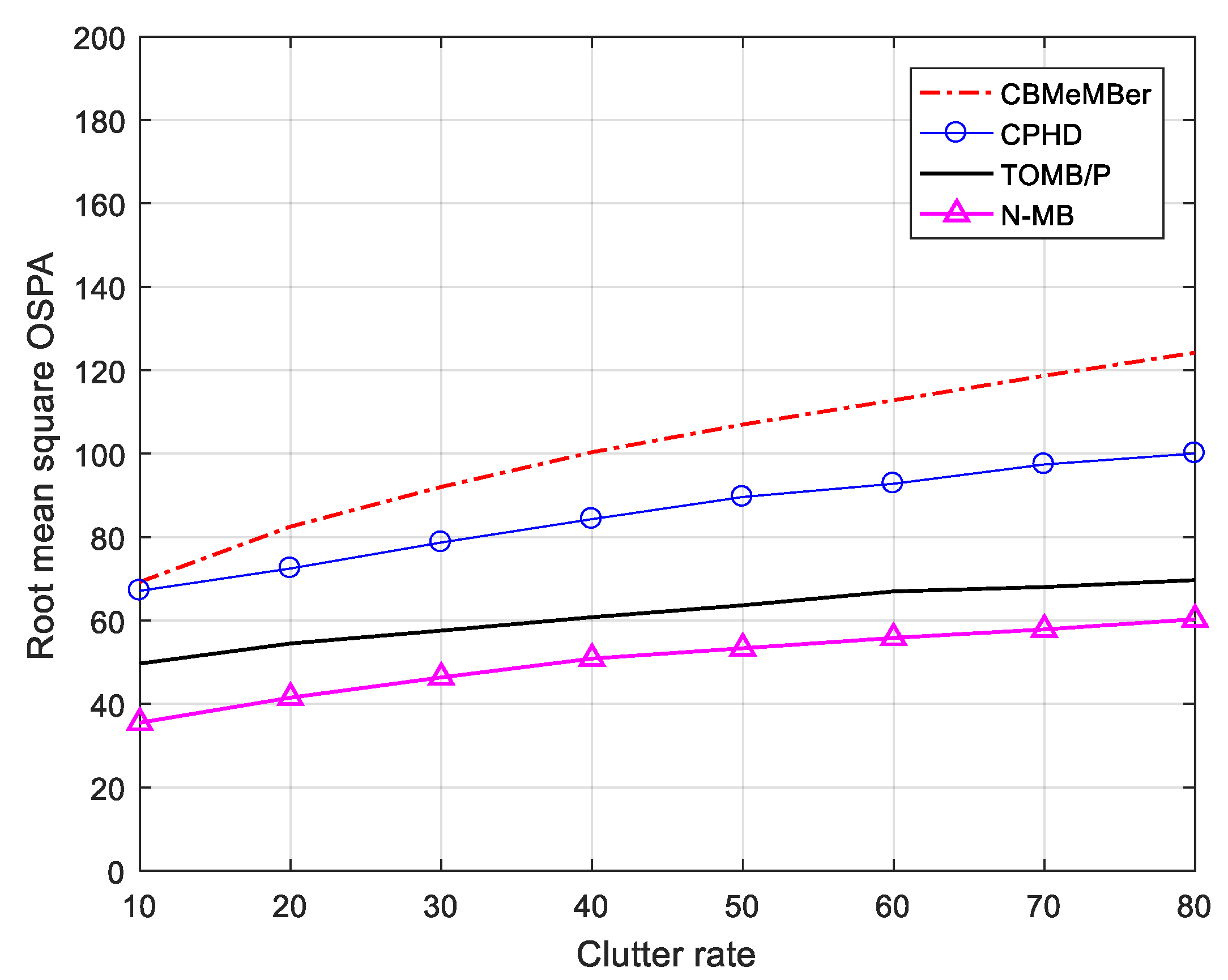
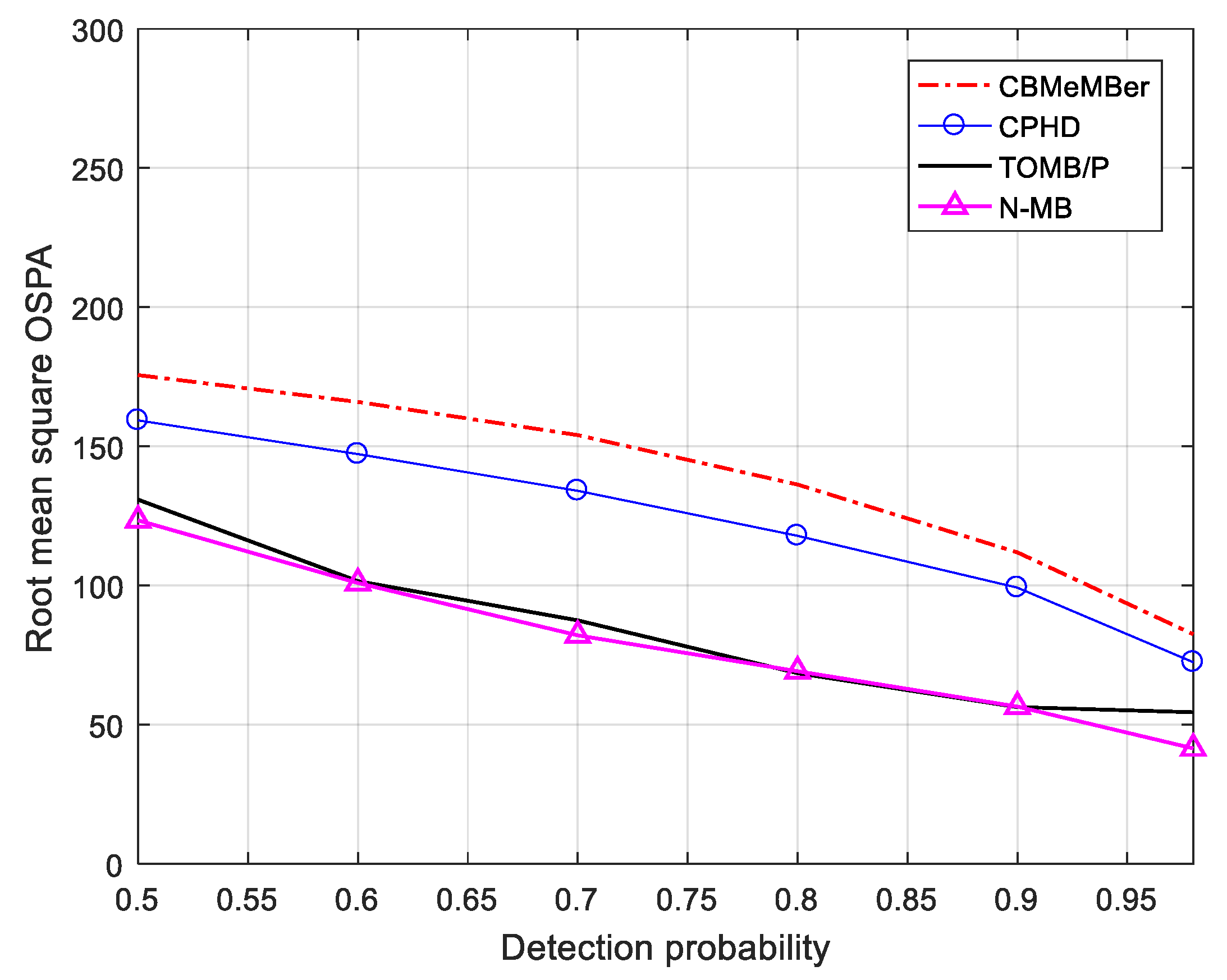
In Figure 5, we give the averages of 200 MC trials for the RMS OSPA distance for the CBMeMBer, CPHD, TOMB/P, and N-MB filters for various clutter rates from ${\lambda }_C=10$ to ${\lambda }_C=80$. In Figure 6, we give the results for various detection probabilities from $p_D=0.5$ to $p_D=0.98$. As expected, the OSPA error increased with the increased clutter rates and a lower detection probability. Overall, these results showed that the N-MB filter had a better performance compared to the other filters. The performance of the CBMeMBer filter was greatly influenced by the increased clutter rate

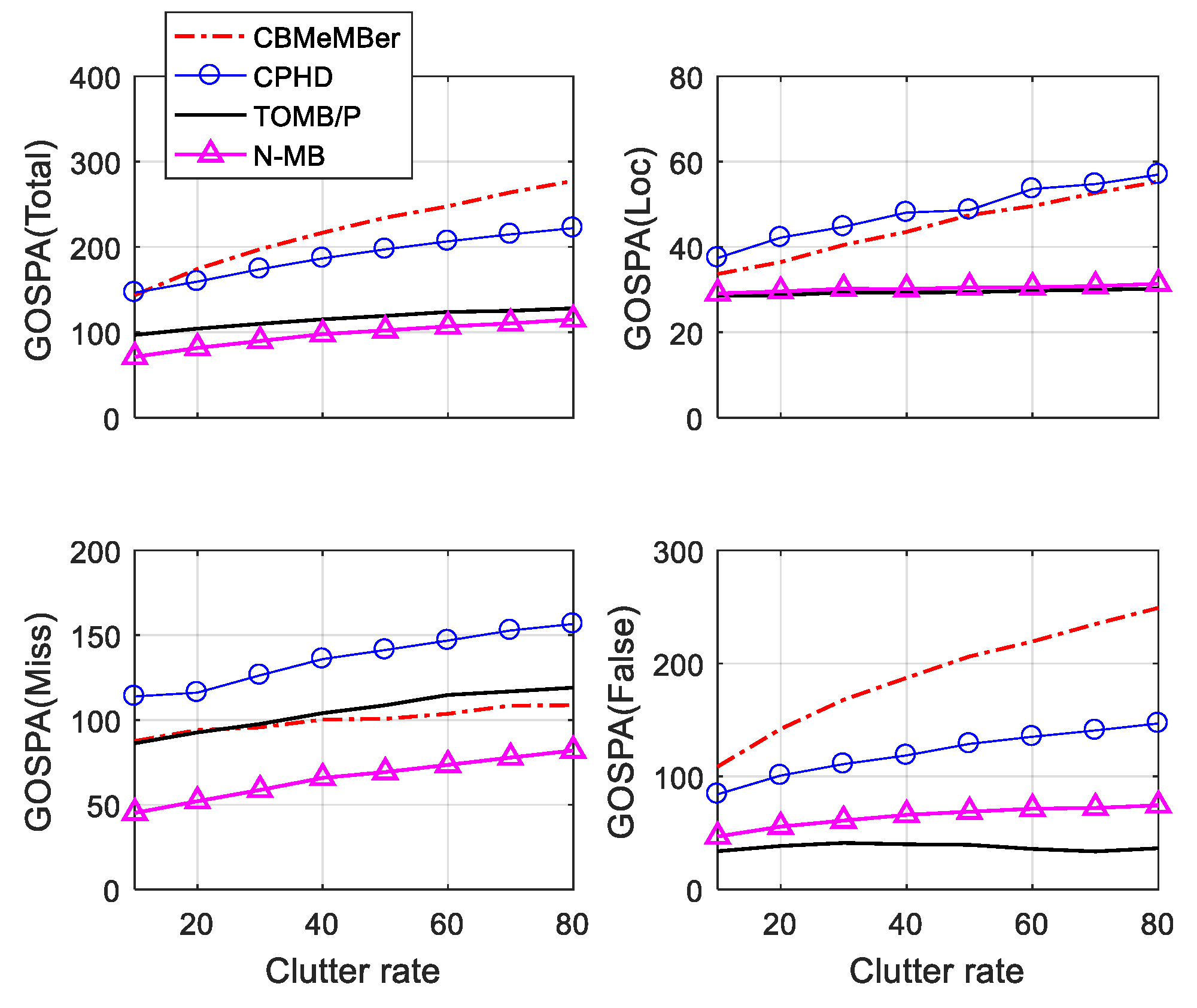
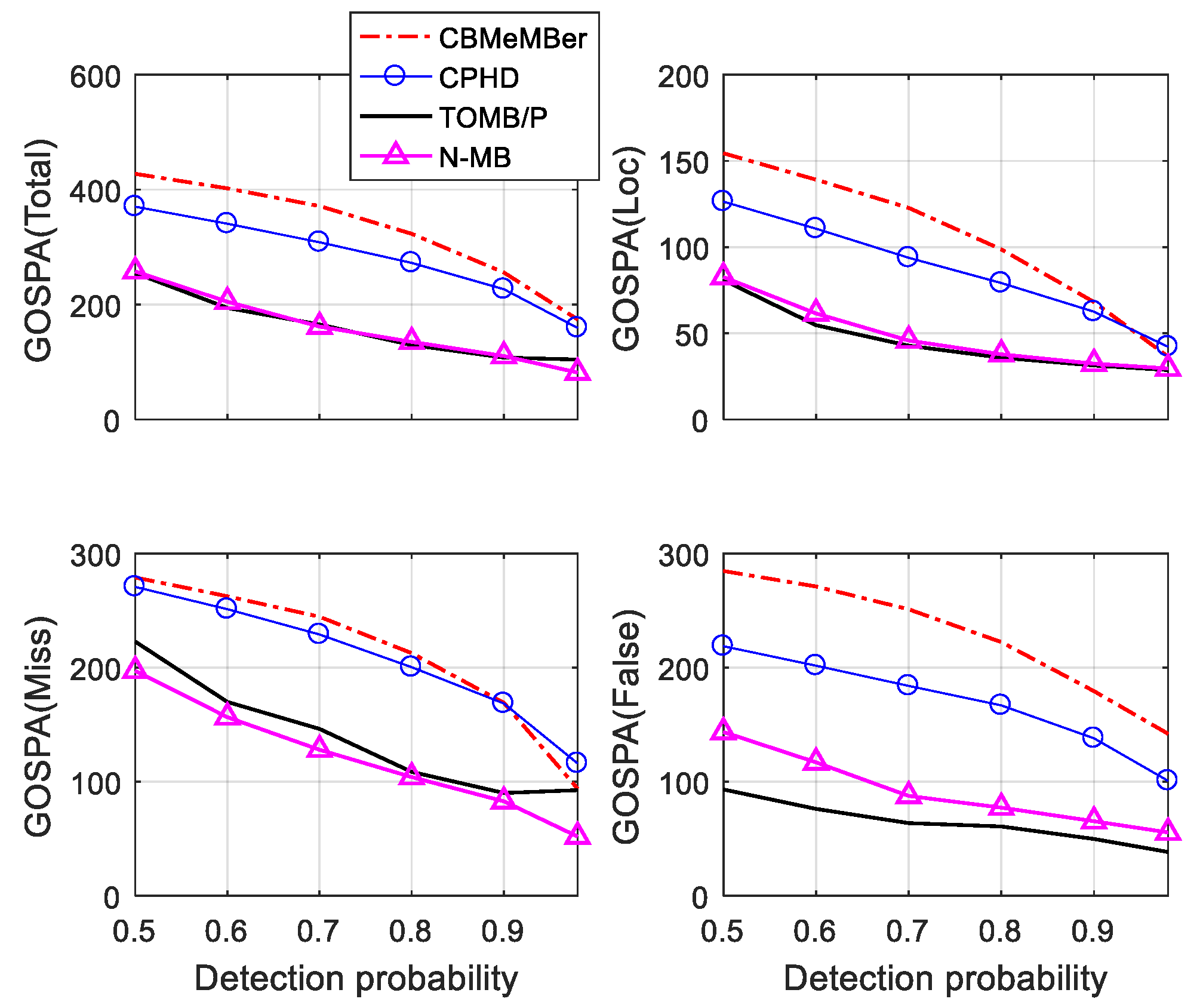
Although OSPA is a good method for measuring the performance of RFS-based MTT filters, we do not know whether the difference in performance of OSPA error comes from a better detection ability, a lower number of false targets, or a lower number of missed targets, which is key information regarding the analysis of filters. As mentioned in Section 5.2, we employed decomposed GOSPA components to verify the performance of filters in terms of location estimations, false estimations, and missed estimations. The RMS OSPA/GOSPA error averaged over all time steps of the filters in different situations are given in Figure 7 and Figure 8. These results prove that the N-MB filter had a similar performance to the TOMB/P filter regarding location accuracy, but outperformed the latter in evaluation of missed targets. The N-MB filter was more sensitive regarding initializing birth tracks; however, this feature meant the N-MB filter produced more false estimates. Overall, the N-MB filter outperformed the TOMB/P filter, especially in the high signal-to-noise environment. Again, the CBMeMBer filter showed its efficient performance in environment with a high signal-to-noise ratio and low clutter intensity, but the performance degraded dramatically in challenging environments.

5.4. Comparison with the LMB Filter

As summarized in Section 3.3, the proposed N-MB filter has a similar structure with the LMB filter, while it has a straightforward prediction step because the N-MB filter was derived based on the theory of PGFls and functional derivatives, while the LMB filter is based on approximating the GLMB density. An efficient implementation method that combines the prediction and update steps of the LMB filter is proposed in Mahler [23], which avoids the complex calculation burden of the prediction step. We compared the time-averaged GOSPA error and computation times (seconds) of the proposed N-MB filter and the LMB filter [23] in different situations, and the results are given in

Table 1. Comparison with the LMB filter.

$\left({\mathit{p}}_{\mathit{D}},{\mathit{\lambda }}_{\mathit{C}}\right)$	N-MB					LMB
	Time (s)	GOSPA	G-Loc	G-Miss	G-False	Time (s)	GOSPA	G-Loc	G-Miss	G-False
$\left(0.98,10\right)$	11.18	71.32	29.12	45.17	46.89	11.95	72.04	29.06	44.62	48.51
$\left(0.98,40\right)$	11.91	97.97	30.14	65.81	66.02	11.96	97.35	29.99	65.38	65.59
$\left(0.98,80\right)$	13.27	115.09	31.38	81.97	74.44	11.99	114.81	31.46	81.31	74.71
$\left(0.7,10\right)$	21.49	143.99	41.95	111.46	80.94	18.91	154.81	42.57	128.89	74.46
$\left(0.7,40\right)$	28.60	180.66	51.42	141.56	99.77	20.07	199.82	51.14	168.29	94.81
$\left(0.7,80\right)$	56.11	293.81	99.86	233.75	147.34	23.43	332.24	91.76	295.15	121.85

. Both filters employ the gating technique, which is widely used in many papers [15,16,22].

Intuitively, the proposed N-MB filter had a similar performance to the LMB filter in high signal-to-noise environments. However, the N-MB filter had a more stable performance in more challenging environments (low signal-to-noise environments with a high clutter intensity). In contrast, a serious leak-tracking problem occurred in the tracking results of the LMB filter when applied in challenging environments.

6. Conclusions

Although the CBMeMBer filter was cardinality balanced, the derivation of which removes the second approximation employed in the original MeMBer filter [3]. It employs the first approximation in Mahler [3], which assumes that measurements are well-separated in the surveillance region. A filter based on this approximation cannot be applied in an environment with high clutter intensity. Moreover, the approximation of a high detection probability is required in the derivation of the CBMeMBer filter; therefore, the filter cannot be applied in the low signal-to-noise environment.

In this paper, we derived a novel-structured MB filter based on PGFl theory and unlabeled RFSs. The proposed filter removed the assumptions utilized in deriving the MeMBer filter. Thus, the filter performed well in the low signal-to-noise and high clutter density environments. Compared to filters based on a GLMB distribution, the proposed filter did not extract explicit tracks for targets. The theory of tracking based on sets of trajectories [35] was utilized to solve this problem. Various simulation results showed that the proposed filter outperformed the LMB filter in low signal-to-noise environments with a little higher computational cost.