1. Introduction
Concomitant with the progressive growth of computing power and communications bandwidth, the size and number of communications-related datasets have also increased in many applications such as telecommunications, social networks, military, etc. [
1,
2]. Massive multiple-input multiple-output (Massive MIMO) technology is an example of such important applications, especially as applied to fifth-generation (5G) wireless communication systems with high data-rate requirements [
3]. It is necessary to process the obtained data in an efficient sampling method in order to extract valuable information about the parameters of the received signals from the increasingly large covariance matrices, which are typically too large and complex for effective manipulation with classical sampling methods [
4,
5,
6].
Estimating direction or angle of arrival (DoA/AoA) parameters has been given the most attention, particularly in far-field signal applications, in which the wavefront of the signal may be treated as being planar [
7]. Radar systems [
8], public security [
9] and emergency call location [
10] are examples of these applications. Additionally, in wireless mobile communication systems, when AoA of the desired user and interference signals are correctly estimated, an adaptive beamforming technique can be applied to emphasise the gain towards the desired signal suppressing the noise and interference signals [
11,
12]. Direction-finding systems face different challenges, caused by the propagation environment, for instance, time-varying nature of the propagation environment, low number of snapshots and the multipath propagation environment [
13,
14]. Moreover, the receiving signals usually suffer from the fading nature of the channels, which causes a poor Signal-to-Noise Ratio (SNR).
Capon’s Method [
15], Multiple Signal Classification (MUSIC) [
16] and Estimation of Signal Parameters via Rotational Invariance Technique (ESPRIT) [
17] are common methods that deal with the AoA estimation problem. Although these methods can provide good estimation, they are infeasible with large-dimension matrices since they need inverse or matrix decomposition operations to solve the problem. Alternatively, a Propagator Direct Data Acquisition (PDDA) method can find the AoAs directly from the observed data matrix without the need to calculate the inverse of the Covariance Matrix (CM) or apply the Eigen/Singular Value Decomposition (E/SVD) approach [
18]. Instead, the PDDA method calculates the cross-correlation vector that represents the cross-correlation between the observed data from the first sensor and the other sensors. Bayesian Compressive Sensing (BCS) theory has been utilised with array signal processing for several investigations [
19,
20]. BCS theory supposes that it is possible to recover signals from fewer measurements if certain conditions are satisfied, as presented in compressive sensing MUSIC (CS-MUSIC) [
21] and subspace-augmented MUSIC (SA-MUSIC) [
22,
23].
Sparse Signal Reconstruction (SSR) has also emerged as a candidate for the AoA problem, to recover signals from a limited number of snapshots and improve robustness to noise compared with conventional techniques [
24]. An algorithm based on compressive sensing theory called Sparse Bayesian Learning/Inference (SBL/SBI) was proposed recently for sparse signal recovery [
25]: with this algorithm, the signal recovery is constructed from a Bayesian perspective while the sparsity data is applied by supposing prior known sparse distributions of the arrival signal for all measurements. Generally, in this method the matrix elements are supposed to be precisely known; regrettably, this hypothesis is invalid when the array manifold suffers from imperfections [
26] or when perturbations of the matrix elements are taken into account [
27]. An Off-Grid Sparse Bayesian Inference (OGSBI) technique was proposed in [
28], by merging the quantisation error problem for point sources and the BCS theory. The quantisation error is taken as real-valued and assumed to be uniformly distributed. The off-grid AoA refinement can be performed optimally if the coarse AoA estimates are in the correct number and all within the trust region [
24,
29]. To satisfy these conditions and obtain off-grid AoA refinement, large numbers of initial bias hampers and earlier iterations are required, and this, in turn, increases the computational burden and execution time.
This work proposes two new AoA methods to estimate the directions of the incident signals on an antenna array. The first is a Reduced Uniform Projection Matrix (RUPM) method for AoA estimation; the second is an efficient and low complexity method, representing the Root version of the Uniform Projection Matrix (Root-UPM) method. The Root-UPM estimates the AoAs by finding the locations of roots of the produced projection matrix instead of looking for the locations of peaks in the pseudo-spectrum. An efficient sampling methodology to choose the positions of these columns was undertaken to determine the optimum strategy for maximising the estimation resolution without increasing the computational complexity. The Uniform Sampling Matrix (USM) methodology is adopted here to adjust the distributions of spacings between the sampled columns in order to increase the separation distance between the eigenvalues of the sampled columns and also to maximise the aperture size of the sampled matrix. This distribution was chosen as being a realistic set to investigate the reduction of data processed in the PM while still giving valid AoA information and facilitating a significant reduction in computational overhead. The chosen methodology also has an additional benefit as it reduces the dependency on the signal time series between the adjacent sample columns, which, in turn, enhances robustness to noise. Therefore, the directions of the incident signals can be determined efficiently with a lower number of snapshots in the presence of poor SNRs.
The rest of the paper is organised as follows:
Section 2 models AoA estimation problem with an arbitrary array geometry. The methodology of the projection matrix construction is given in
Section 3. The idea and working principle of the proposed angle of arrival algorithms, including the uniform sampling methodology, are given in
Section 4. The theoretical analysis and the complexity of computations are derived and presented in this Section as well. Simulation results, discussions, and comparisons are displayed in
Section 5. Finally,
Section 6 summarises the results and sets out conclusions.
2. Angle of Arrival Estimation Model with Arbitrary Array
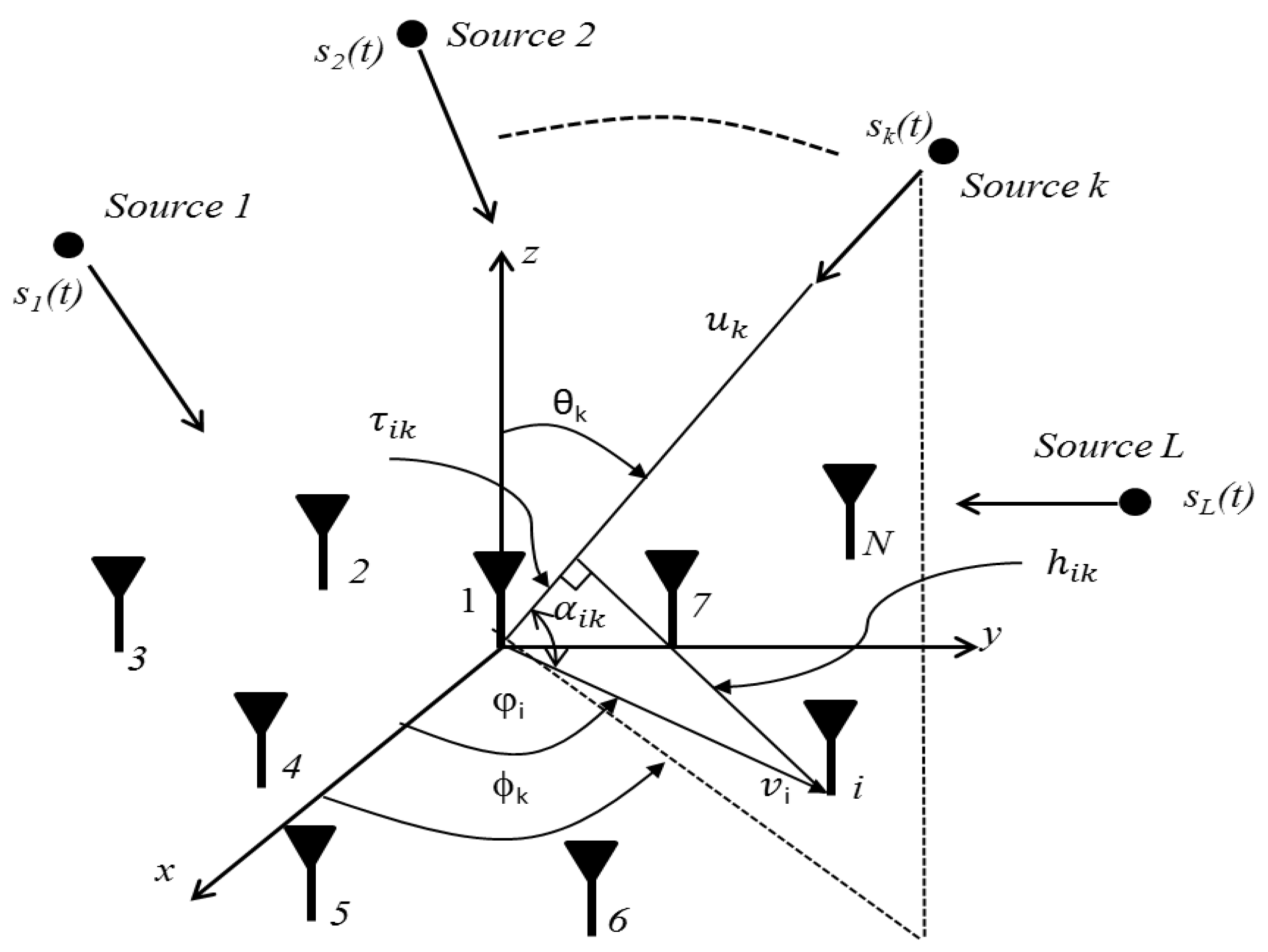
For generality, a 3D arbitrary antenna array geometry consisting of M elements is adopted and used to model the AoA estimation problem. L sources are assumed located in the far-field and sending L narrowband signals, which incident on this array from different elevation angles (
θj) and azimuth angles (
ϕj) incident, as shown in
Figure 1. The incident signals are measured by the M sensors and then down-converted to the baseband level in order to process them digitally and finding the AoAs of the incoming signals. The vector of the received data, including the additive noise, is described below.
where:
is a modulated signal.
is the Additive White Gaussian Noise (AWGN).
is a steering matrix that includes L steering vectors as described below:
To derive the steering vector of the
kth plane wave that incidents on the above array, one needs to define the unit vector that includes the elevation and azimuth angles for such
kth incident signal as follows:
Here,
and
are the unit vectors for Cartesian coordinates. The second step is to define the unit vector that represents the distance between a reference element and the other antenna elements as follows:
Here,
denotes the separated angle between the x-plane and the positions of each element. Next, the produced angle between the
and
vectors for the ith element and with respect to a reference element (i.e., element 1, see
Figure 1) needs to be computed utilising the dot product between these vectors as given below:
The total set of
due to L plane waves incident on M sensors can be given as a matrix with (M × L) dimension:
The time delay of the kth incident signal on M antenna elements with respect to the original reference element,
, as shown in
Figure 1, can be calculated as follows:
The corresponding matrix that contains the time delays of L impinging plane waves on M antenna elements is:
The angular phase difference (
) is presented below:
The phase difference matrix that includes the full set of
can be described as follows:
Then, the array steering vector that can be applied to any array configuration can be given below;
3. The Projection Matrix Construction
The conventional sub-set sampling approach for projection matrix construction uses a crude slice of the CM data, and it is to be expected that such sampling is non-optimal. To construct a projection matrix, consider there are M elements receive L signals at N times, then, the collected data matrix,
, can be given as follows:
The array covariance matrix (
) can be computed by applying the expectation process to the received data matrix as follows [
18]:
where
is the matrix of steering vectors defined in (2),
is the (L × L) source signal correlation matrix,
,
is the noise variance,
is the (M × M) identity matrix, and ()
H represent the conjugate transpose operation.
When the signals sources are travelling from one location to another with time (i.e., the arriving signals are time-varied), it’s incident direction on the antenna array will alter with time as well and this, in turn, will vary the steering vectors matrix. Then, the computations are dependent upon timed measurements of the arrival signal. Practically, it is difficult to obtain the actual CM and, thus one needs to use the sample-average estimated array input matrix to construct
as follows [
30]:
This matrix,
, includes the information of L signals and therefore, the highest rank-L matrix to M under both the Frobenius and spectral norms can be represented by [
31]:
In other words, the columns of this decomposition are projections of L columns of M onto the span (
: 1 ≤
i ≤
L). Then, the projection matrix can be calculated, based on the signal subspace matrix as follows [
32]:
Here,
is the signal subspace matrix that contains the information of L dominated eigenvalues
. Now, one can construct the spatial spectrum of the MUSIC method using the below formula [
33]:
Based on (17), the projection matrix uses the signal eigenvectors, and consequently, the CM must be decomposed to obtain these eigenvectors, which will cost a high computational burden. Alternatively, L rows/columns of the CM can be exploited to be fundamentally the equivalent of the Hilbert-Schmidt or Frobenius norms without the need to decompose the CM. The over-riding problem, however, is to find a method of picking an L-subset of rows/columns of M ∈
CM×L so that projecting onto their span is almost as good as projecting onto span (
: 1 ≤
i ≤
L), but with avoiding any increase in the complexity of computations [
4]. To proceed, assume that there is L plane waves incident on an array consisting of M elements, hence the size of the CM is (M × M). We need to sample C columns, where L < C < M: as described below:
Let us assume the required sample matrix from
be assigned the symbol
as follows:
where
∈
CM×L is the signal subspace sampled matrix, having dimensions (M × L). However, there is no optimum criterion or method to select the positions of these rows/columns. The criterion that has been used in the state-of-art heretofore has been largely based on the information in the first L rows/columns within the CM [
34,
35,
36]. We will call this criterion the classical method and the sampled matrix will be termed
, where
, such that
represents the set of columns in the matrix
and
is the set of column numbers. The chosen columns set
from the matrix
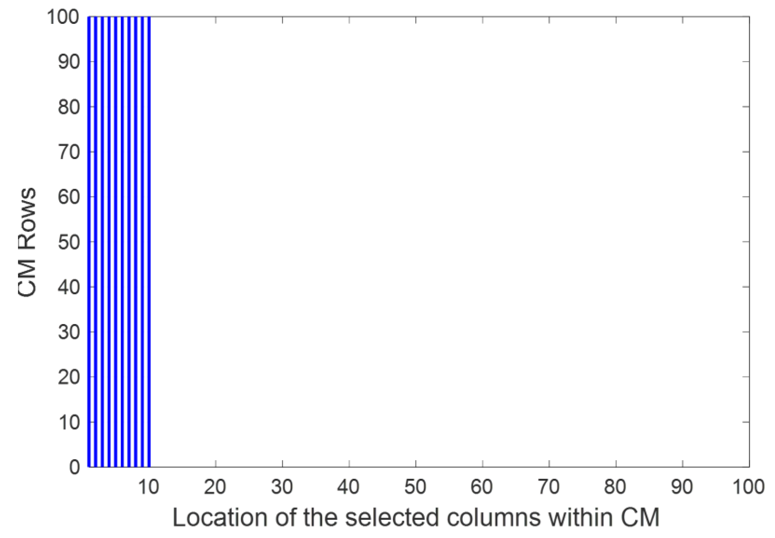
, using the classical sampling methodology is given by;
The distribution and locations of these columns under this method can be represented conceptually as shown in
Figure 2; the blue lines represent the locations of the selected columns in the CM.
The projection matrix can be computed as follows [
37]:
Then, the spatial spectrum of the PM method can be formed using the following formula [
32].
The performance of this algorithm is significantly based on the matrix. Thus, a new sampling technique is given in the next section to improve and enhance the AoA estimation accuracy.
4. The Proposed Angle of Arrival Methods
The selected sampling matrix
gives some picture of that interdependence structure. The critical question is: to what extent does the selected sample,
, present a correct representation of the signal subspace matrix? Thus, the methodology of sampling the covariance matrix and selecting the
columns has significant impacts on the estimation resolution, as stated by [
4]. Volume sampling is the selection
l-subsets of the rows/columns of a certain matrix with probabilities proportional to the squared volumes. It was first introduced in [
38] in the context of low-rank approximation of matrices. This means that rows or columns from the matrix can be selected essentially at random to obtain a dimension-reduced problem with necessarily the same norm as the original. The behaviour of the largest L eigenvalues is based mainly on the method of sampling the CM. To this end, a new sampling matrix approach is proposed to expand the array aperture of
in the next sub-section.
4.1. The Reduced Uniform Projection Matrix (RUPM) Method
In a previous works [
32,
37], the impact on the estimation accuracy and the Probability of Detection (PoD) of AoAs of the number of sampled columns (size of the sampled matrix) that was used in the projection matrix construction has been analysed and investigated. It was demonstrated that an increase in the number of the sampled columns leads to increases in the estimation resolutions and PoD. However, the computational complexity of the projection matrix construction is increased with increasing size of the sampled matrix. Thus, it is crucial to utilise an efficient sampling method that can extract sufficient information about the signal parameters without introducing new problems such as grating lobes, angle estimation ambiguity and increase of the computational burden.
Instead of the straightforward approach shown in
Figure 2, it is intuitively reasonable to consider a more distributed approach to the allocation of the columns of the subspace matrix. As a first trial, a uniform sampling distribution was applied to extract the received data in the CM efficiently. Thus,
was constructed using a uniform structure instead of utilising the first L columns of
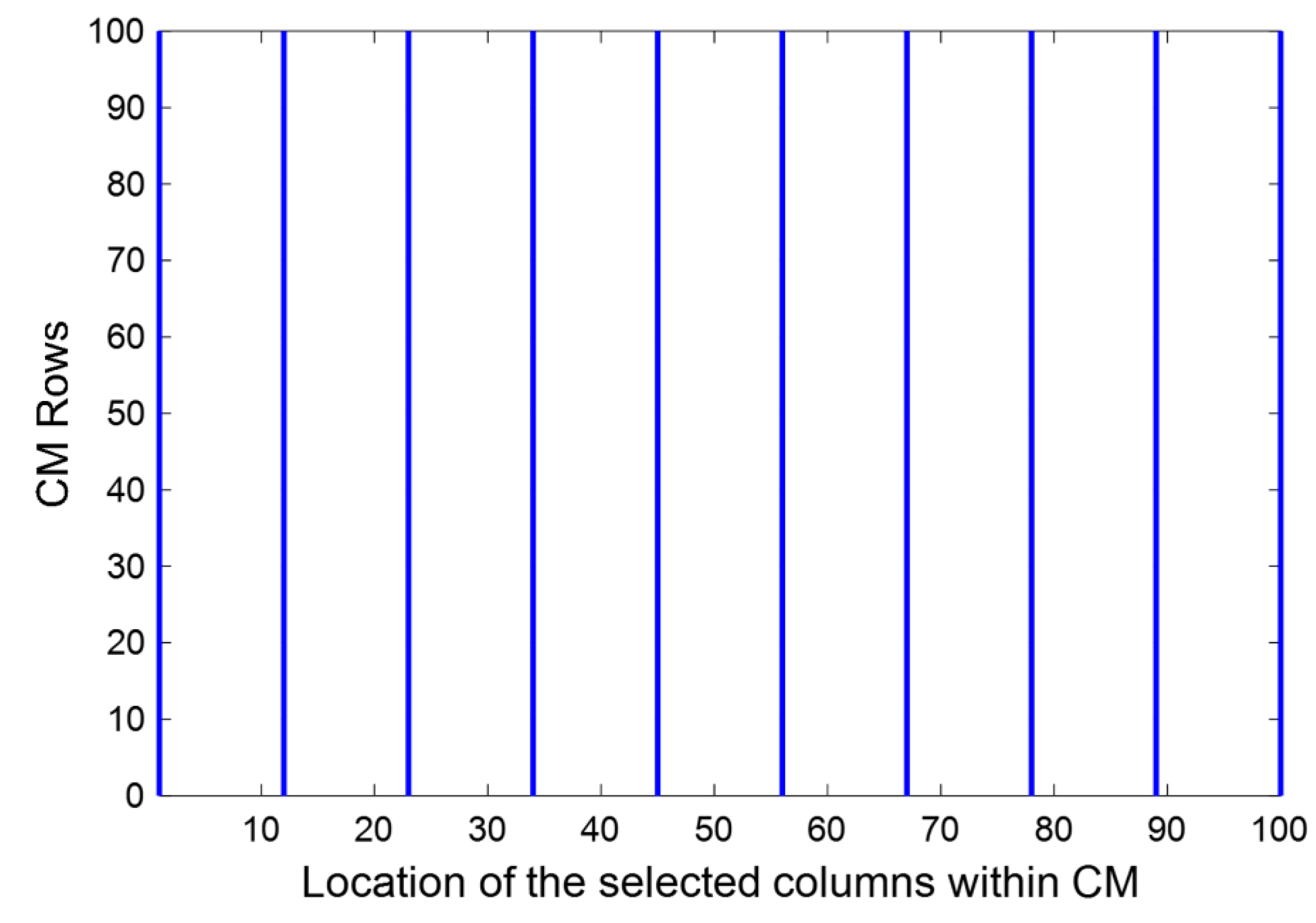
. In this structure, the distance between the L columns was set uniformly: this can be defined by the specification of a system of subsets of the product (M × C) as given in (23). The methodology of selected CM columns based on this formula can be shown in
Figure 3. It is clear from this figure that the size of the obtained aperture array of
is wider than that with
as illustrated in
Figure 2.
It can be also observed that the distance between the adjacent columns of is larger than with . This, in turn, will minimise the correlation on the signal time series between the sampled columns and remove the dependency with the steering vector, hence eliciting the individual AoAs.
Based on the uniform selecting criterion, the Uniform Projection Matrix (UPM) can be computed as follows:
is the computed projection matrix based on the uniform sampling methodology.
To reduce the complexity of computations, it is suggested to reduce the size of the above matrix from (M × M) to (M × G); this can be accomplished by multiplying as follows:
where
is M × G identity matrix and defined as:
G is a pre-defined number, and to ensure this algorithm is applicable for an arbitrary antenna array and suitable for 2D and 3D estimation, its value should be in this range: 2 ≤ G ≤ M. Now, the pseudo spectrum of the Reduced UPM (RUPM) approach can be formed as follows:
4.2. The Root-UPM Method
From a computational complexity point of view, searches to the roots that corresponding to AoAs instead of looking to the location of peaks in the pseudo spectrum is much less computational. Thus, the root version of the UPM method is presented here to reduce the computational burden due to the grid searching stage. The Root-UPM technique can be described as follows:
where
. By taking the denominator of (28), the Root-UPM becomes the following formula:
Here,
is the entry in the mth row and the nth column of
. For simplicity, one can convert the above double summation into single summation by assuming
. The range of
is limited by
and
, i.e.,
. Hence, the above equation becomes as follows:
where
is the propagation constant, d is the separation distance between the adjacent elements,
is the direction of the incident signal within the elevation plane, and
represents the sum of the
th diagonal elements of the matrix
. A polynomial
that is equivalent to
can be defined as follows:
where
. Since the spectrum of
should have L peaks, then, the
spectrum should contain L nulls. To this end,
should include L zeros located on the unit circle. The other zeros of the polynomial
will be located far from the unit circle.
The result of (31) represents the roots that may be corresponded to the peaks of the pseudo spectrum of the UPM method. Every root could be complex and defined by the polar notation:
where
denotes to phase angle of
.
In the absence of noise, the actual zeros are located exactly on the diameter of the unit circle, thus, the condition of the root magnitude being equal to one (i.e.,
) is applied. However, this assumption is difficult to satisfy in practical applications as the arriving signals typically contain a certain amount of noise and, therefore, the zeros may be located slightly away from the diameter of the unit circle. To this end, it is necessary to place a threshold around them such as 0.90 to 1.1, in order to determine the number of roots (i.e.,
). The arrival angles can then be computed as follows
Here,
represents the direction of the incident signals that obtained from the root location (i.e.,
).
4.3. Flow Chart for the Proposed AoA Methods
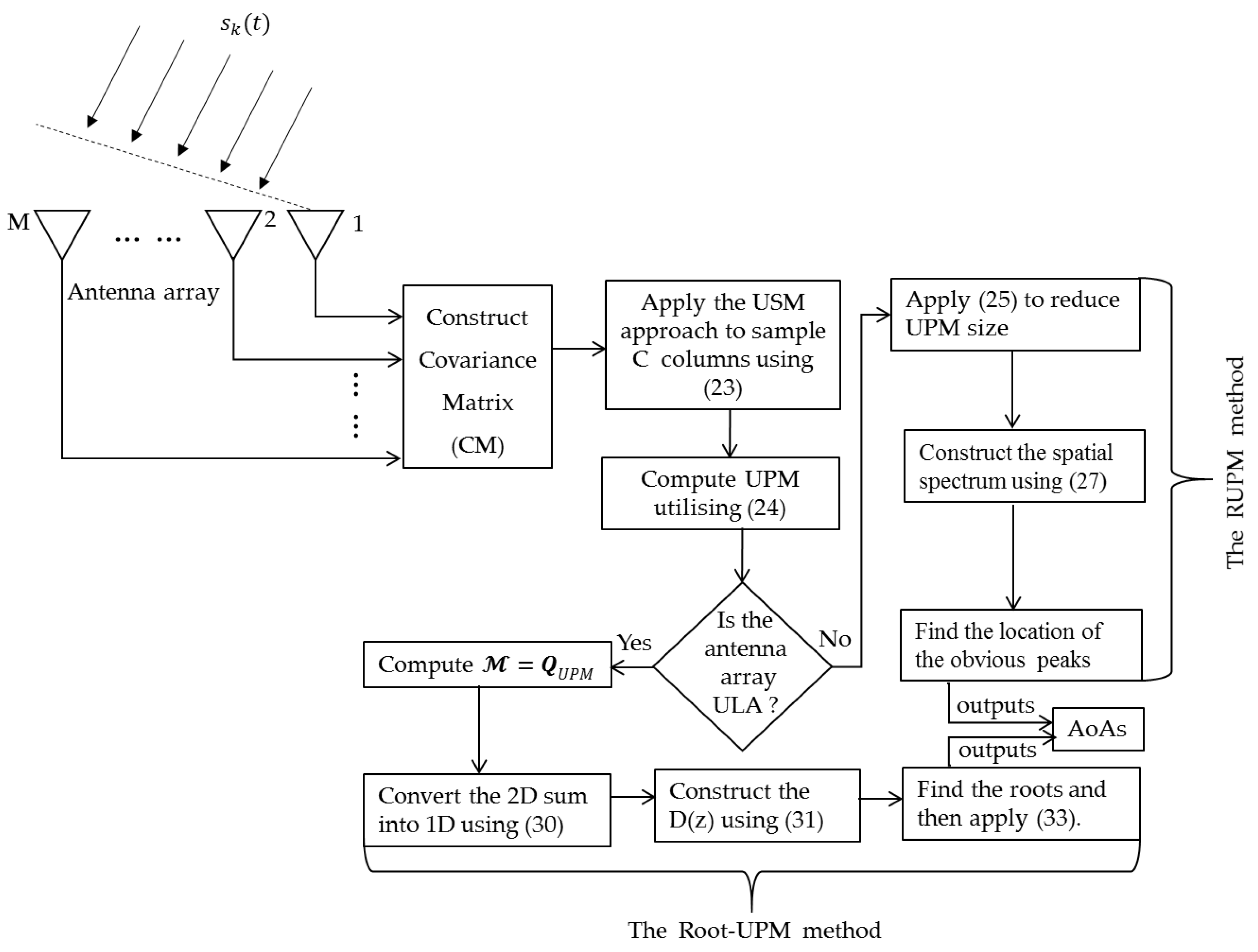
The whole signal processing steps needed to implement the RUPM and Root-UPM methods started from measuring signal by an antenna array until obtaining the AoA of the incident signals can be summarised in
Figure 4.
It can be seen from this diagram both methods share the first three stages namely: CM construction, applying the USM methodology and UPM construction. After that, each method has a different route to determine the direction of the received signals. If the geometry of the used array is Uniform Linear Arrays (ULAs), both RUPM and Root-UPM can be applied in the signal processing stage to find the AoAs. However, it is recommended to apply the Root-UPM method as it much faster and less computational complexity than the RUPM algorithm and also can give better estimation accuracy. If the 2D or 3D array has been used such planar, circular, cubic, etc. then only RUPM can be applied since the Root-UPM is applicable only for ULA.
4.4. Theoretical Analysis of DOFs
For the AoA estimation, the objective is the determination of the number of nulls of the array factor instead of the number of maxima. It is assumed for this operation that the number of sample columns ‘C’ used to conclude the CM should satisfy the equality C = L + 1. With the classical sampling methodology, the array factor can be formed based on the first C picked columns as follows:
where
, by multiplying both sides of (34) by
, this yields:
By subtracting equation (35) from (34) results in:
The above equation represents the number of nulls of the array factor due to the classical sampling criterion. With further simplifications, the above equation can be given as follows:
From (37), it can be seen that the maximum number of nulls is C-1 where these nulls are used to point peaks toward the incident signals. To justify any advantage in terms of angular precision with the proposed methodology compared to the conventional one, the possible produced nulls will be computed using the proposed sampling methodology. For uniform sampling, the space between each two adjacent sampled columns is set as U = round (M/L), where U is the uniform sampling factor. Based on the uniform sampling criterion, the array factor can be given by:
By multiplying both sides of (38) by
yields:
Subtracting (39) from (38) results in:
where
.
Simplifying the above equation, it can be presented as follows:
The array nulls can occur when the numerator argument of (41) is equal to
Tψ/2 =
. Therefore, the number of produced nulls utilising the USM approach can be given as follows:
The number of produced nulls using (42) is T, and this number is much more than that obtained by (37). The number of nulls using the USM approach compared the that produced with the conventional methodology can be calculated by dividing (41) on (37) as follows:
Based on the proposed distribution of the selected number of columns, the resolution can be varied when the weights are changed even though the degrees of freedom are equal for both approaches. The ratio of the number of nulls can play a substantial role in adjusting the AoA accuracy to separate closely spaced signals incident on the array.
4.5. Computational Complexity Analysis
Most of the localisation applications look for implementing a low complexity AoA method, especially with large array sizes. The reduction in the quantity of calculations of any system makes the processing system efficient with less consumption power [
39]. Typically, the computational complexity of an AoA method consisting of three main stages. Firstly, constructing the CM, which costs O (M
2N). After that, based on the used method where some AoA algorithms need to decompose the CM, which requires O (M
3) or computes the projection matrix that needs to O (M
2C) arithmetic operations, etc. [
18,
40]. It should be noted with massive MIMO, the burden of O (M
3) will suffer from infeasibly high computational complexity. Finally, most of the current AoA system includes the searching grid step in order to construct the spatial spectrum and then finding the location of the produced peaks. The computational load of this stage is based mainly on three parameters namely: the matrix dimension, the size of the searching step (
), and the angular range of scanning (
). In the present work,
was assumed to cover the angular range [−90° 90°] and
= 0.5°, then
.
The total computational complexity of the proposed AoA methods based on the above arguments have been calculated and compared with common and well-known AoA techniques as given the
Table 1.
5. Numerical Simulations and Discussions
To evaluate the potential advantages of the proposed AoA method, computer simulations over a wide range of scenarios were undertaken and the results compared with several AoA approaches. Four main types of test are undertaken; firstly, a numerical example comparison using various techniques is presented to show the performance of each algorithm in identifying the angles of arriving signals. Secondly, the execution time is calculated to measure the speed and complexity of computations. In the third scenario, the estimation accuracy of the proposed methods is compared with several commons AoA techniques based on SNR variations, and finally, it is investigated with a different number of collecting the data matrix. In the last two scenarios, the Average Root Mean Square Error (ARMSE) of AoAs was computed as follows:
where
K is the number of Monte Carlo trials,
and
are actual and estimated angles, respectively.
5.1. Inter-comparison: Numerical Example
A numerical scenario was implemented with different incident AoAs to illustrate the principles developed. A ULA consisting of M = 32 with d = 0.5λ was considered and used to receive ten narrowband signals (L = 10) from sources located in the far-field. The number of measurements that assumed to construct the CM was set as N = 100 and SNR at the array output was set at 10 dB. The searching step angle is
0.5°. The directions of the ten plane waves are
= [32° 36° 39° 65° 100° 142° 149° 154° 164° 175°] and indicated by red circles. Three of the received signals were postulated to be incident at closely similar angles
= {32° 36° 39°}, in order to investigate the ability to resolve and detect directions of signals under this circumstance. In addition, five signals are incident at angles widely distant from the broadside direction,
= {142° 149° 154° 164° 175°}, some of them close to each other. The RUPM and Root-UPM methods in addition to four other different AoA techniques, are considered here and used to estimate the directions of the incident signals. The reduction projection matrix parameter of the RUPM method is set to G = 5. For the OGSBI, For the Root-SBL and OGSBI methods, the maximum number of iterations and the tolerance error are set at 200 and 0.001, respectively, while the other simulation parameters are set as same as those presented in [
28,
45]. The performance comparison of these algorithms is illustrated in
Figure 5.
As shown, the RUPM estimated the directions of all incident signals by producing ten obvious peaks towards them. The Root-UPM has also detected all the arrival angles without the need to construct the spatial spectrum, which reduced the computational burden, memory storage and the execution time extremely. For, the Projection Matrix (PM) based on the classical sampling criterion, propagator, OGSBI algorithms detected the directions of only seven signals. The Root-SBL failed to identify two plane waves. This confirms the strength and effectiveness of the proposed techniques and demonstrates that the way of sampling obtained date has a significant effect on the signal estimation parameters.
5.2. The Execution Time Comparison
The running time of the proposed RUPM and Root-UPM methods were compared with the execution time of four different algorithms, namely: PM; propagator; OGSBI; Root-SBL methods. The main simulation parameters are adjusted as follows: M = 32; N = 100; L = 10; G = 5;
0.5° and
= 722. A MATLAB code for each method has been written and the tic and toc functions were used to measure the execution time. The specifications of the PC that was adopted and used in this simulation are processor: Intel(R) Core (TM) i7-4790 CPU @ 3.6 GHz, with 32 GB installed RAM and the type of the operating Windows 8.1. A MATLAB simulation programme for each method was run under the same computer situations with one hundred iterations; the total time of execution of each technique was recorded and given in
Table 2.
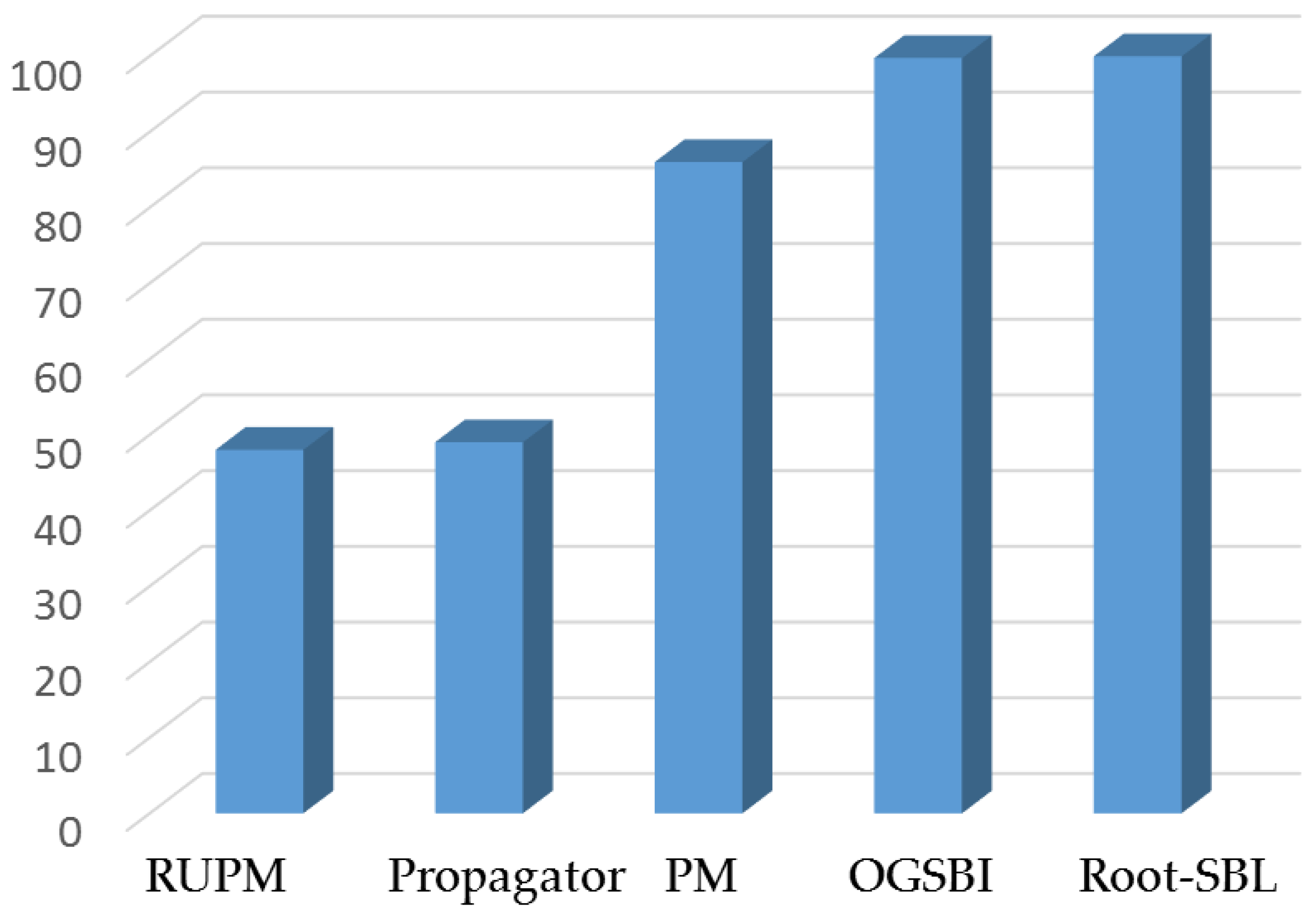
As illustrated, the Root-SBL and OGSBI are the slowest algorithms and need extremely execution time to achieve the estimation process. The execution time of the PM method is reasonable and much less than the two previous algorithms. The needed execution time for the propagator and RUPM techniques is approximately the same three times less than the time, which needed for PM method. The Percentage of the Reduced Execution Time (PRET) using the Root-UPM was computed and compared with other algorithms based on the following formula:
To compute the percentage of the reduce execution time using the Root-UPM compared to the RUPM, propagator, PM, OGSBI and Root-SBL methods, one can substitute the running time of these methods (see
Table 2) in the t
comp separately to obtain this percentage. The reduced execution time percentage of the Root-UPM method compared to other techniques is shown in
Figure 6.
As illustrated, the running time of the Root-UPM method is 48% and 49% less than the RUPM and propagator techniques, respectively. However, the running time of the Root-UPM approach is 86%, 99.74% and 99.96% less than the PM, OGSBI and Root-SBL methods, respectively. The reason of the slow convergence of the OGSBI and Root-SBL methods is because its computational complexity not only based on the number of snapshots and antenna elements but also on the other parameters such as the maximum number of iterations and tolerance error, which are required to find the optimum solution.
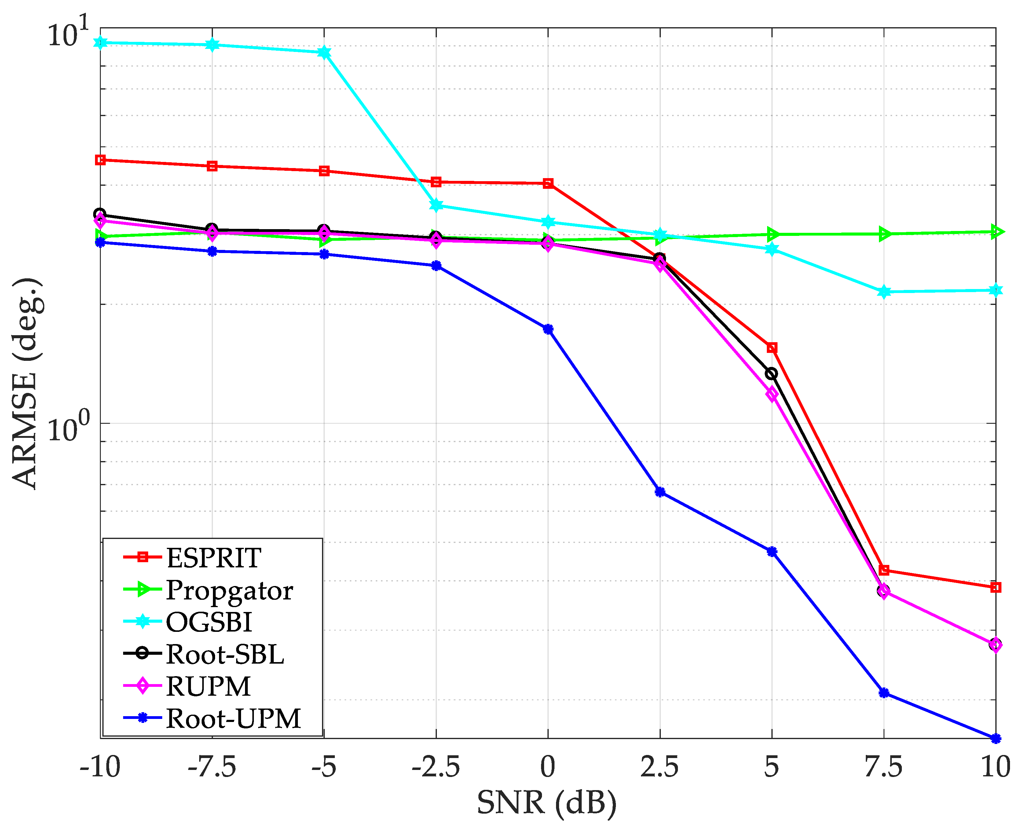
5.3. Comparisons Based on SNR Variations
The SNR represents the ratio of the received signals power to the power of the additive noise (i.e.,
) and this ratio plays an essential role in the performance estimation of the AoA method. Thus, the impact of the SNR on the estimation accuracy is tested and compared by assuming the SNR varies from −10 dB to 10 dB in 2.5 dB increments. Ten plane waves (L = 10) from different directions postulated as incident on a ULA consisting of M = 32 sensors with d = 0.5λ. One hundred snapshots were considered and used to construct the received data matrix. The same angles of arrival that assumed in
Section 5.1 are applied in this scenario for all techniques equally to ensure a fair comparison. The ARMSE for each SNR was computed and then plotted, as shown in
Figure 7. As depicted, the proposed methods (i.e., RUPM and Root-UPM) gives a better estimation resolution compared to other AoA techniques. It can be observed that the Root-UPM gives the best estimation accuracy among the compared methods through the whole the tested SNR range with the least computational burden as justified in
Section 5.2. The performance of the RUPM is better than OGSBI, propagator and ESPRIT algorithms and comparable to the Root-SBL approach. However, the complexity and the execution time of the RUPM is much less than Root-SBL method as verified in
Section 5.2.
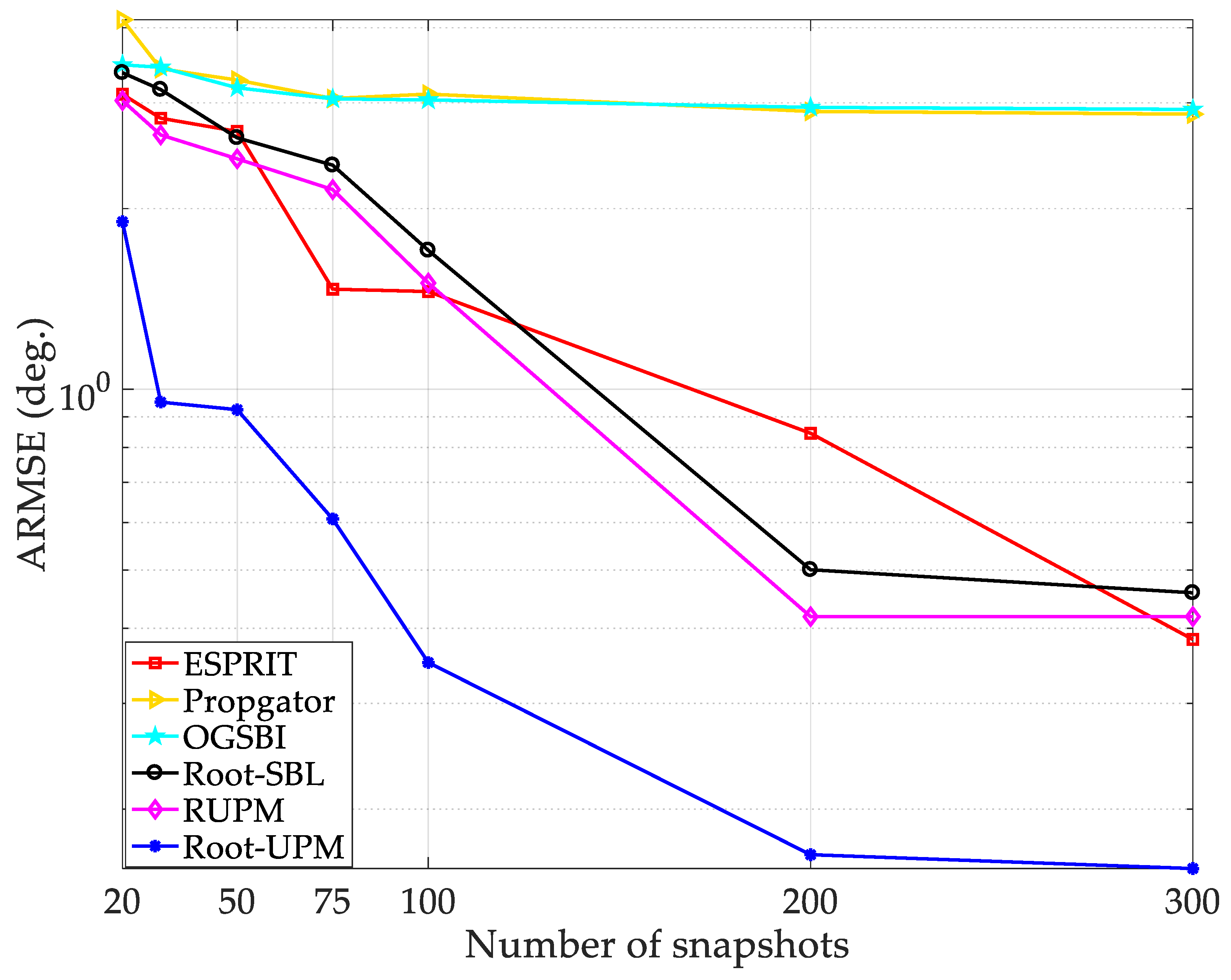
5.4. Comparisons Based on Different Number of Snapshots
The last scenario compares the effect of the performance of the RUPM and Root-UPM methods with four popular AoA techniques based on different numbers of snapshots. Seven different numbers of snapshots were used: N = (20, 30, 50, 75, 100, 200, 300). The other simulation parameters were set to be the same as those given in
Section 5.2 except that the SNR was set at 5 dB. The ARMSE of each method was computed and then plotted, as shown in
Figure 8. It is clear that the proposed methods present better estimation accuracy over the simulated range of snapshot numbers, in comparison with the other methods. The Root-UPM provides the best estimation resolution compared to the simulated methods through the whole testing range. Furthermore, the RUPM approach gives approximately better direction estimation accuracy than the ESPRIT and Root-SBL techniques with significant improvements compared to the propagator and OGSBI algorithms.
This verifies that the sampling approach to select subsets of rows/columns inside the CM and the way of constructing the projection matrices has a significant positive impact on the estimation accuracy. It is relevant to note that these improvements were accomplished with the low computational load as proved in
Table 1 and
Table 2. The reason for the OGSBI gives poor estimation is this method based on sparse signal reconstruction to deal with such an off-grid AoA estimation problem. The approximation quality is deteriorated when the number of the iteration is not enough to construct the off-grid AoA refinement, which, in turn, corrupt the discretised sampling grid. Thus, the location of constructed gird can be far to the true AoA, which yields a highly significant error. However, performing large numbers of initial bias hampers and earlier iterations will increase the computational burden and execution time significantly.
6. Conclusions
In this work, accurate and essay to implement AoA methods called uniform sampling matrix and its root version have been proposed to find the arrival angles of the incident signals on an antenna array. The proposed methodologies were chosen to test a realistic range of distributed positions of rows/columns to be selected within the CM and use this to create the projection matrix. The bases of these approaches and the working principle were presented and modelled. It was found that these approaches have a significant impact in retaining all of the relevant information while reducing the correlation between the columns of the sampled matrix and minimising the dependency with the steering vector and thus facilitated elicitation of the individual AoAs. The theoretical analysis showed that the proposed methodology could produce many more nulls, namely CU+U-1, compared to the classical sampling approach, which produced only C-1 nulls. A numerical example was given to prove the theoretical claims where the proposed approaches were able to detect and identify all the ten AoAs. A Monte Carlo simulation was performed with different values of SNR and the number of snapshots to illustrate the enhancement that could be realised by the use of the proposed AoA methodologies. The simulation results showed that the proposed two methods gave significant improvements in the estimation error and the probability of detection of the angles of arrival, compared to the other AoA algorithms. The computational complexity and execution time are calculated and compared as well. The results showed that the reduced execution time percentage of the Root-UPM compared to the propagator, PM, OGSBI and Root SBL methods are 49%, 86%, 99.74% and 99.96%, respectively.

 ,
, 


