Estimating the Information Source under Decaying Diffusion Rates

Abstract

Recently, as arising from online social network services such as Facebook and Twitter, people are more actively using social networks to exchange their new information. In this consideration, finding the information source becomes one of the indispensable and useful tasks in detecting a malicious agent and an influential person in the networks. A seminal work by Shah and Zaman in 2010 showed that the detection probability cannot be beyond 31% even for regular trees if time goes to infinity. From the study, extensive researches have been done for this problem, whose major interests lie in constructing an efficient estimator and providing theoretical analysis on its detection performance. However, most of the works assumed the homogeneous diffusion rate of the information, where the diffusion rate does not change at all times over the network. In practice, it is reported that information has a lifetime and it becomes less attractive over time. In this paper, we study the problem of detecting the information source when the diffusion rate decreases by the distance from the source in the network. As a result, we obtain analytical detection performance of Maximum Likelihood Estimator (MLE) and validate our theoretical findings over the regular tree, random and real-world networks.

1. Introduction

In the era of big data that came with the rapid development of the Internet, information spread is universal including the propagation of infectious diseases, the technology diffusion, the computer virus/spam infection on the Internet, and sharing popular topics by the Facebook. Information source estimation is the problem that identifies the initial seed node of the diffused information in the network. This is clearly of practical importance, because harmful diffusion can be mitigated or even blocked, e.g., by vaccinating humans or installing security updates. In the seminal work by Shah and Zaman [1], it is shown that in the regular tree topologies, the detection probability cannot be above 31% under Maximum Likelihood Estimator (MLE), and even worse, in other realistic topologies such as Facebook graphs, scale-free graphs and Internet Autonomous System (AS) graphs, the detection probability is less than 5% under the MLE-based heuristic due to a complex structure of networks. Since then, extensive research attention for this problem have been paid for various network topologies and diffusion models [1,2,3,4,5,6,7,8], whose major interests lie in constructing an efficient estimator and providing theoretical analysis of its detection performance. Prior work directly or indirectly conclude that this information (We use the terms “information” and “rumor” interchangeably through the paper.) source finding turns out to be a challenging task unless sufficient side information or multiple diffusion snapshots are provided. There have been several research efforts which use multiple snapshots [6] or a side information about a restricted suspect set the true source belongs [7], thereby the detection performance is significantly improved. Another type of side information is the one obtained from querying, i.e., asking questions to a subset of infected nodes and gathering more hints about who would be the true information source [9,10]. However, most of the works have focused on the homogeneous diffusion rate which means that the rate is same at all times over the network. This is impractical because it is reported [11] that information has a lifetime and it becomes less attractive over time. In other words, the diffusion power will be reduced over time or the number of distance (hops) to the source as in Figure 1. In this paper, we consider that the diffusion rate of information decays with respect to the distance from the source (We do not consider the diffusion rate decays over time due to some mathematical intractability for analyzing the performance.). Under this scenario, we try to find the source by using a proper estimator.

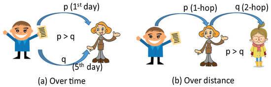
Figure 1. Examples of decaying diffusion rate of information. (Initial diffusion rate p and decayed rate q: (a) over time and (b) over distance.)

To the best of our knowledge, this is the first work to consider the decaying diffusion rate on the information source detection problem.

Our main contributions are summarized in what follows.

• First, we use the MLE to find the source for decaying diffusion and show that the MLE is same as that of the homogeneous diffusion rate of information if the diffusion decays with respect to the distance from the source. This implies that the MLE of our model also has the same graphical centrality property called rumor center in [1]. This enables us to analyze the detection performance for the decaying rate scenario.
• Second, we define two exponential decaying models: $\left(a\right)$ Simple exponential decay and $\left(b\right)$ Generalized exponential decay. The simple exponential decay is a kind of light tail distribution, but the generalized exponential decay covers light and heavy tail distribution in the sense of the decaying pattern. We then obtain the closed-form of detection probability of the MLE when the underlying graph is a regular tree for both decaying models. Different to the prior result in [1], the detection probability is larger than zero in the line graph and there is a non-neglectable improvement of detection for any degree of a regular tree.
• Third, we consider the case that the decaying model parameter is hidden for two decaying models above. This is a more realistic scenario because knowing the exact parameter of the model is not easy in practice. To do that, we first derive MLE to estimate this parameter and show that it needs exponential computing time. Hence, we design a heuristic estimation algorithm for the true parameter by using the diffusion snapshot information, appropriately.
• Finally, we validate our theoretical result for the regular tree using the MLE and for over popular random graphs (Erdös-Rényi, scale-free and small-world graphs) and real-world networks (US-power grid, Facebook and Wiki vote) using the heuristic Breath-First-Search (BFS) estimator. As a result, we see that the detection probability can be above 80% for the regular tree and it can be above 30% if the diffusion rate decays, whereas it is about 20% without decaying in the Facebook graph.

The remainder of this paper is organized as follows. Section 2 discusses related literature. In Section 3, we introduce the information diffusion model and estimator. The theoretical results for detection performance of decaying rate will be presented in Section 4, and the corresponding proof will be provided in Section 5. In Section 6, we depict the simulation results and conclude the paper in Section 8. The detailed proof will be presented in the Appendix A.

2. Related Work

The research on information source detection has recently received significant attention. We divide them into the following three categories: $\left(i\right)$ single source estimation, $\left(ii\right)$ multiple sources estimation, and $\left(iii\right)$ hiding and seeking the sources.

$\left(i\right)$ Single source estimation. The first theoretical approach was done by Shah and Zaman [1,2,3], which introduced the metric called rumor centrality—a simple topology-dependent metric for a given diffusion snapshot. They called a node that has maximum rumor centrality by rumor center as a MLE. They proved that the rumor centrality describes the likelihood function when the underlying network is a regular tree and the diffusion follows the Susceptible-Infected (SI) model, which is extended to a random graph network in [2]. Zhu and Ying [4] solved the source detection problem under the Susceptible-Infected-Removed (SIR) model and took a sample path approach to solve the problem, where the Jordan center was used, being extended to the case of sparse observations [5]. There were several attempts to boost up the detection probability. Wang et al. [6] showed that observing multiple different epidemic instances can significantly increase the detection probability. Dong et al. [7] assumed that there exist a restricted set of source candidates, where they showed the increased detection probability based on the Maximum a Posterior Estimator (MAPE). Choi et al. [8] showed that the anti-rumor spreading under some distance distribution of rumor and anti-rumor sources helps to find the rumor source by using the MAPE. Choi et al. [9,10] studied the effects of querying to finding the source and showed how many queries are sufficient to achieve a target detection probability. The authors in [12,13] introduced the notion of set estimation and provided the analytical results on the detection performance. Luo et al. [14] considered the problem of estimating an infection source for the SI model, in which not all infected nodes can be observed.

$\left(ii\right)$ Multiple sources estimation. Different from the single source estimation, multi-source estimation requires inferring the set of source nodes. Despite the difficulty of the problem, some prior studies tried to solve this problem by appropriate set estimation methods. Prakash et al. [15] proposed to employ the Minimum Description Length (MDL) principle to identify the best set of seed nodes and virus propagation ripple, which describes the infected graph most succinctly. They proposed a highly efficient algorithm to identify likely sets of seed nodes given a snapshot and show that it can optimize the virus propagation ripple in a principled way by maximizing the likelihood. Zhu et al. [16] proposed a new source localization algorithm, named Optimal-Jordan-Cover (OJC). The algorithm first extracts a subgraph using a candidate selection algorithm that selects source candidates based on the number of observed infected nodes in their neighborhoods. Then, in the extracted subgraph, OJC finds a set of nodes that cover all observed infected nodes with the minimum radius. Considering the heterogeneous SIR diffusion in the ER random graph, they proved that OJC can locate all sources with probability one asymptotically with partial observations. Ji et al. [17] developed a theoretical framework to estimate rumor sources, given an observation of the infection graph and the number of rumor sources.

$\left(iii\right)$ Hiding and seeking the source. As opposed to finding the information source from a given snapshot of the epidemic, hiding the corresponding source approach also has been studied. Fanti et al. [18] first considered this problem and proposed an Adaptive Diffusion (AD) for the information spreading protocol. They showed that AD is near-optimal for hiding the source as well as maximizing the information spreading on the regular tree structures. Luo et al. [19] considered a problem that an information source tries to hide with maximizing the spread of its information, whereas the network adversary seeks the source, simultaneously. They formulated this problem by a game theoretic model and showed that a Nash Equilibrium (NE) exists under some mild condition of the game.

To the best of our knowledge, our paper is the first to quantitatively consider the decaying of diffusion power, which is more realistic scenario compared to the homogeneous diffusion rate. We obtain that the source can be found more easily when the diffusion rate decays with respect to the distance from the source for the real world graphs as well as tree structure.

3. Model and Estimator

We consider an undirected graph $G=(V,E),$ where V is a countably infinite set of nodes and E is the set of edges of the form $(i,j)$ for $i,j\in V$. Each node represents an individual in human social networks or a computer host in the Internet, and each edge corresponds to a social relationship between two individuals or a physical connection between two Internet hosts [9]. As an information spreading model, we consider a SI model as in [1,2,4], where each node is in either of two states: susceptible or infected. In this model, once a node has the information, it keeps it forever, i.e., it does not allow for any nodes to recover. All nodes are initialized to be susceptible except the information source, and once a node i has information, it is able to spread the information to another node j if and only if there is an edge between them. We denote a random variable ${\tau }_{ij}$ by the time it takes for node j to receive the information from node i if i has it. We denote $v^{\ast }\in V$ by the information source, which acts as a node that initiates diffusion and denote $V_N\subset V$ of N infected nodes under the observed snapshot $G_N\subset G$. In this paper, we consider the case when G is a regular tree and our interest is when the sufficient time has passed, as done in many prior work [1,2,6,7]. Even though the real network may not be the regular tree with high probability, it is shown that many random graphs can be approximated by regular tree due to locally tree-like structure [20]. Note that most of the works have focused on the case that all edge $e=(u,v)$ for node pair u and v have same diffusion rate (or probability), say $\lambda >0$. However, in this work, we assume that the diffusion rate of all edge $e=(u,v)$ for node pair u and v is a function of distance from the information source $v^{\ast }\in V$. We assume that ${\tau }_{ij}$ are independent and have an exponential distribution with parameter ${\lambda }_h$ where h is the number of hops of node i from the source. Hence, the diffusion rate only depends on the distance to the source in the graph. Further, we assume that a diffused information has a message about how many hops (h) passed from the source (Using this message, each infected node spreads the information to its neighbors under the diffusion rate ${\lambda }_h$).

Maximum Likelihood Estimator. As an estimator of the source, we consider a MLE for the observed graph (snapshot) $G_N$ when there are N infected nodes in the network:

$$\begin{array}{cc}\hfill {\widehat{v}}_{\mathtt{ml}}& =arg{\displaystyle \underset{v\in G_N}{max}}P(G_N|v),\hfill \end{array}$$

(1)

i.e., the MLE is the node that maximizes the likelihood $P(G_N|v)$ of the diffusion snapshot $G_N$. Instead of direct computing the likelihood, which is quite difficult due to heterogeneous diffusion rate, we consider the following proposition that guarantees a useful graphical characterization of the MLE.

Proposition 1.

Let ${\mathcal{V}}_{ml}$ be a set of MLEs (We consider the set of MLEs because it can be multiple nodes.) for the homogeneous diffusion rate and let ${\mathcal{V}}_{ml}\left(h\right)$ be the set of MLEs for (1) on the regular tree. Then we have ${\mathcal{V}}_{ml}={\mathcal{V}}_{ml}\left(h\right).$

The proof of Proposition 1 will be presented in Section 5. This proposition indicates that for a given regular tree, the MLE of our decaying diffusion model is the same to that of the homogeneous diffusion rate. Consequently, we have the same graphical property of “rumor center” as described in [1], which is one of the graph centrality concepts. To see more details, we let $T_u^v$ be the number of nodes in the subtree rooted at node u, assuming v is the root of the tree $G_N$ (see [1] for details). Then the rumor center has the following property.

Corollary 1.

Under d-regular tree G, for a given observation $G_N$ with N infected nodes, the node v is a MLE of (1) if and only if $T_u^v\le N/2$ for every neighbor u of v.

For a comparative purpose, we first present the detection probability of MLE for the homogeneous diffusion rate [2] as follows:

Lemma 1

([1]). Under d-regular tree G, let $P({\widehat{v}}_{\mathtt{ml}}=v^{\ast })$ be the detection probability of MLE then ${lim}_{t\to \infty }P({\widehat{v}}_{\mathtt{ml}}=v^{\ast })=0$ for $d=2$ and for $d\ge 3$

$$\begin{array}{c}\hfill {\displaystyle \underset{t\to \infty }{lim}}P({\widehat{v}}_{\mathtt{ml}}=v^{\ast })=1-d\left(1-{\mathrm{I}}_{1/2}\left(\frac{1}{d-2},\frac{d-1}{d-2}\right)\right),\end{array}$$

(2)

where ${\mathrm{I}}_x(\alpha ,\beta )$ is the incomplete Beta function (The incomplete Beta function ${\mathrm{I}}_x(\alpha ,\beta )$ is the probability that a Beta random variable with parameters α and β is less than $x\in [0,1]$, whose form is ${\mathrm{I}}_x(\alpha ,\beta )=\frac{\Gamma (\alpha +\beta )}{\Gamma \left(\alpha \right)\Gamma \left(\beta \right)}{\int }_0^x{t}^{\alpha -1}{(1-t)}^{\beta -1}dt$ where $\Gamma (·)$ is the standard Gamma function [1].) with parameters α and β.

Using Lemma 1, one can check that the detection probability for MLE under the homogeneous diffusion rate is at most $0.307$ in the asymptotic case for d-regular trees. In the following section, we define our interesting decaying models and obtain the detection probabilities under these models.

4. Main Results

In this section, we first obtain the asymptotic detection probability (when $t\to \infty$) for two decaying models with known model parameters. Next, we consider a case that the model parameter is hidden (unknown) so that we need to estimate it. To do that, we suggest a simple and efficient parameter estimation algorithm.

4.1. Probability of Correct Detection of MLE

As a first decaying model, we define a simple decay function as follows. To do this, we introduce a decaying parameter $p>1$, which indicates how much the diffusion rate will be decay by the number of hops to the source. Using this, we have the following definition.

Definition 1

(Simple Exponential Decay). Let ${\lambda }_0$ be the initial diffusion rate from the information source $v^{\ast }$. We call the rate function ${\lambda }_h\left(p\right)=\frac{{\lambda }_0}{p^h}$ by simple exponential decay w.r.t. the source with the decaying parameter $p>1$.

Using this definition, we first obtain the detection probability of the MLE when the underlying graph is a line. To do that, we let $P({\widehat{v}}_{\mathtt{ml}}\left(p\right)=v^{\ast })$ be the detection probability of the information source by the MLE for the simple exponential decay. Then we have the following result.

Theorem 1.

For the line graph with the decaying parameter $p>1$, the detection probability of the information source by the MLE when t goes to infinity is given by

$$\begin{array}{c}\hfill {\displaystyle \underset{t\to \infty }{lim}}P({\widehat{v}}_{\mathtt{ml}}\left(p\right)=v^{\ast })=\frac{1}{M\left(p\right)}\left(1+\frac{1+p}{2p}\right),\end{array}$$

(3)

where $M\left(p\right):=2{\sum }_{k=1}^{\infty }{p}^{\frac{-k(k+1)}{2}}+2.$ Furthermore, if $p\le 1,$ then ${lim}_{t\to \infty }P({\widehat{v}}_{\mathtt{ml}}\left(p\right)=v^{\ast })=0.$

In this result, we check that if $p=2$, the detection probability is larger than $7/16$ by using an integral approximation of $M\left(p\right)$. Further, we see that if p increases the detection probability also increases. This is a significant enhancement of detection compared to that of the homogeneous diffusion rate where the detection probability is zero for the line graph [2].

Next, we will obtain the source detection probability for d-regular tree ($d\ge 3$) as follows.

Theorem 2.

Under d-regular tree G $(d\ge 3)$, if $p\ge d-1$, the MLE can detect the source with probability one as t goes to infinity, i.e.,

$$\begin{array}{c}\hfill {\displaystyle \underset{t\to \infty }{lim}}P({\widehat{v}}_{\mathtt{ml}}\left(p\right)=v^{\ast })=1.\end{array}$$

(4)

This result indicates that for the d-regular tree ($d\ge 3)$, if the decaying rate of the information is larger than $d-1$, the MLE can detect the source almost surely even though the time goes to infinity. This is because the tendency of great decaying makes the snapshot of diffusion more dense with respect to the source so that the MLE can find it easily (Since the MLE is a rumor center under the decaying model, the estimator has the largest centrality of the graph.). Next, we introduce a more general exponential decaying model where the decay level is parameterized by r from the simple exponential decaying to homogeneous rate by one parameter in what follows:

Definition 2

(Generalized Exponential Decay). Let ${\lambda }_0$ be the initial diffusion rate of the information source $v^{\ast }$. We call the rate function ${\lambda }_h(p,r)$ by generalized exponential decay with respect to the source if

$$\begin{array}{c}\hfill {\lambda }_h(p,r)=\frac{{\lambda }_0}{p^h}(1+r{\displaystyle \sum _{l=1}^h}{p}^{h-l}),\end{array}$$

(5)

where $0\le r\le p-1$ is the decay level.

We see that this form is parameterized by r. For example, if $r=0$ then it becomes the simple exponential decay as in Definition 1. If $r=p-1$ then it becomes ${\lambda }_0$ which is the homogeneous diffusion rate. We plot the rate function ${\lambda }_h(p,r)$ with various values of parameters $(p,r)$ in Figure 2. Using this, we obtain the following result.

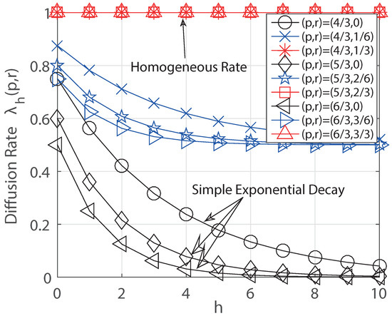
Figure 2. Example of generalized exponential decay. (If $r=p-1$, it becomes a homogeneous rate and if $r=0$, it is a simple exponential decay.)

Theorem 3.

Under d-regular tree G $(d\ge 3)$, let $P({\widehat{v}}_{\mathtt{ml}}(p,r)=v^{\ast })$ be the detection probability of the information source by the MLE under the generalized exponential decay ${\lambda }_h(p,r)$ in (5). If $p=d-1$ then we have

$$\begin{array}{c}\hfill {\displaystyle \underset{t\to \infty }{lim}}P({\widehat{v}}_{\mathtt{ml}}(p,r)=v^{\ast })=1-d\left(1-{\mathrm{I}}_{1/2}\left(\frac{1}{r},\frac{d-1}{r}\right)\right).\end{array}$$

(6)

The result implies that for a given decaying level r, we have the asymptotic detection probability of the MLE as in (6). For example, if $r=0$ then ${lim}_{t\to \infty }P({\widehat{v}}_{\mathtt{ml}}(p,r)=v^{\ast })=1$ which is the result in Theorem 2 and if $r=d-2$ then the detection probability becomes the result in [1] which is the case of the homogeneous diffusion rate.

4.2. Decaying Parameter Estimation

In this subsection, we consider the scenario that the parameter p of the decaying model is hidden because it is often hard to know the exact parameter even though the model is given in practice. In this case, under the decaying model, one can estimate it by the following MLE simply using the current snapshot $G_N.$ To formalize this, we let $\sigma =(v_1=v,v_2,\dots ,v_N)$ be a infection sequence which generates $G_N$ and let $\mathsf{\Omega }(v,G_N)$ be the set of these sequences when v is the source. Then we have

$$\begin{array}{cc}\hfill p_{\mathtt{ml}}& =arg{\displaystyle \underset{p}{max}}P(G_N|p)\hfill \\ \hfill & \stackrel{\left(a\right)}{=}arg{\displaystyle \underset{p}{max}}{\displaystyle \sum _{v\in G_N}}P(G_N|p,v)\hfill \\ \hfill & =arg{\displaystyle \underset{p}{max}}{\displaystyle \sum _{v\in G_N}}\left({\displaystyle \sum _{\sigma \in \mathsf{\Omega }(v,G_N)}}P(\sigma |p,v)\right),\hfill \end{array}$$

(7)

where the equality $\left(a\right)$ is due to the uniform prior of the source. Then, we see that computing the MLE has combinatorial complexity because there are exponentially many infection sequences in $\mathsf{\Omega }(v,G_N)$ with respect to the infected nodes N. Hence, instead of using this, we design an approximation algorithm that guarantees simple and efficient to estimate the true parameter as follows.

Algorithm. We now describe our decaying parameter estimation algorithm, named DPE(K), where K is sampling cost of the algorithm in Algorithm 1. Since we do not have any prior information for the parameter p, we set the estimation range $[p_{min},p_{max}]$, where $p_{min}$ and $p_{max}$ are minimum and maximum values of p, respectively. We set $p_{min}=1$ (i.e., no decaying) in the algorithm. Then, the algorithm first sets $p=p_{min}$ as described in the first line. Next, for each infected node $v\in \mathsf{\Omega }(v,G_N)$, it calculates the rumor centrality $R(v,G_N)$ using the given snapshot information $G_N$ as in [1] (Step 1). To approximate the term ${\sum }_{\sigma \in \mathsf{\Omega }(v,G_N)}P(\sigma |p,v)$ in (7), we consider that the algorithm samples K infection sequences uniformly at random (The uniform sampling indeed gives a simple approximation for the mean of infection probabilities), where K is a fixed constant $K\ge 1$ and computes:

$$\begin{array}{c}\hfill {\overline{P}}_K(\sigma |p,v)={\displaystyle \sum _{i=1}^K}P({\sigma }_i|p,v)/K,\end{array}$$

(8)

where ${\sigma }_i(1\le i\le K)$ is randomly sampled infection sequence on $\mathsf{\Omega }(v,G_N).$ (Step 2). This is regarded as a averaged value of $P({\sigma }_i|p,v)$ in (7). Clearly, we know that many samples (large K) give more accuracy in general. Then, we multiply ${\overline{P}}_K(\sigma |p,v)$ to the rumor centrality $R(v,G_N)$ and we put it into $\overline{R}(v,G_N)$ (Step 3). We next sum these values for all infected nodes and save it to $f\left(p\right).$ We repeat this procedure by increasing $\delta >0$ to the previous value p. Finally, the algorithm compares all values of $f\left(p\right)$ within the range $[p_{min},p_{max}]$ and takes the maximum p as the estimation of decaying parameter, denoted by $\widehat{p}$. We see that the algorithm complexity is $O\left(\max \right\{N,K\left\}\right)$, where N is the number of infected nodes in the graph. We will show how accurate this algorithm as varying K in the simulation section.

Algorithm 1 Decaying Parameter Estimation (DPE(K))

Input: Diffusion snapshot $G_N$, sampling cost K, $p_{min}$, $p_{max}$, increasing step size $\delta$

Output: Estimation parameter $\widehat{p}$

Set the initial decaying parameter $p\leftarrow p_{min}$;

while $p\le p_{max}$ do

for each $v\in G_N$ do

Step1: Compute the rumor centrality $R(v,G_N)$ by a message passing algorithm [1];

Step2: Choose random samples ${\sigma }_i\in \mathsf{\Omega }(v,G_N)$ K times and compute its mean by; $$\begin{array}{c}\hfill {\overline{P}}_K(\sigma |p,v)={\displaystyle \sum _{i=1}^K}P({\sigma }_i|p,v)/K.\end{array}$$ (9)

Step3: Set $\overline{R}(v,G_N)\leftarrow R(v,G_N)·{\overline{P}}_K(\sigma |p,v)$;

end for

Set $f\left(p\right)$←${\sum }_v\overline{R}(v,G_N)$;

$p\leftarrow p+\delta$;

end while

Compute $\widehat{p}=arg{max}_{p}f\left(p\right)$;

Return $\widehat{p}$;

5. Proof of Results

In this section, we will provide the proofs of Propositions and Theorems. All proofs of Lemmas will be provided in Appendix A.

5.1. Proof of Proposition 1

To prove this, it is sufficient to show that under d-regular tree G, for a given observation $G_N$ with N infected nodes, v is a MLE of (1) if and only if $|T_u^v|\le N/2$ for every neighbor u of v from the result in [1]. Let $v\in G_N$ be the node which satisfies this condition and let $u\in G_N$ be a node that has $|T_w^u|>N/2$ for some neighbor node w of u. Then, we will prove $P(G_N|v)>P(G_N|u)$ for all $u\in G_N$ by using a contradiction method. Suppose there exists a node u such that $P(G_N|v)\le P(G_N|u).$ To determine $P(\sigma |v)$ where $\sigma =\{v_1=v,v_2,\dots ,v_N\}\in \mathsf{\Omega }(v,G_N)$ is a infection sequence (permitted permutation of $G_N$), if v is the source, we let $G_k\left(\sigma \right)$ be the subgraph of $G_N$ containing nodes $\{v_1,\dots ,v_k\}$ for $1\le k\le N.$ Then, for every $\sigma \in \mathsf{\Omega }(v,G_N)$ and $\sigma \in \mathsf{\Omega }(u,G_N),$ we have

$$\begin{array}{cc}\hfill P(\sigma |v)& ={\displaystyle \prod _{k=2}^N}P(k^{th}\mathrm{infected}\mathrm{node}=v_k|G_{k-1}\left(\sigma \right),v)\hfill \\ \hfill & ={\displaystyle \prod _{k=2}^N}P\left({\displaystyle \underset{1\le j\le n_{k-1}\left(\sigma \right)}{min}}{\tau }_j=v_k|G_{k-1}\left(\sigma \right),v\right)\hfill \\ \hfill & ={\displaystyle \prod _{k=2}^N}\frac{{\lambda }_j\left(\sigma \left(v\right)\right)}{{\sum }_{j=1}^{n_{k-1}}{\lambda }_j\left(\sigma \left(v\right)\right)}\hfill \\ \hfill & \stackrel{\left(a\right)}{>}{\displaystyle \prod _{k=2}^N}\frac{{\lambda }_j\left(\sigma \left(u\right)\right)}{{\sum }_{j=1}^{n_{k-1}}{\lambda }_j\left(\sigma \left(u\right)\right)}=P(\sigma |u),\hfill \end{array}$$

(10)

where ${\tau }_j$ is the exponential random variable of the jth node at the boundary of the information spread and the inequality $\left(a\right)$ follows from the fact that if we let $L_u:={max}_{s\in G_N}d(u,s)$ then by the decreasing diffusion rate, we have $P(L_u>L_v)>P(L_u\le L_v)$ and this makes $P(\sigma |v)>P(\sigma |u)$ for any permutation $\sigma .$ To see this more rigorously, we see that for any permutation $\sigma \in \mathsf{\Omega }(u,G_N),$ there exists distinct permutation $\sigma \in \mathsf{\Omega }(v,G_N)$ such that $\left(a\right)$ holds $\frac{{\lambda }_j\left(\sigma \left(v\right)\right)}{{\sum }_{j=1}^{n_{k-1}}{\lambda }_j\left(\sigma \left(v\right)\right)}>\frac{{\lambda }_j\left(\sigma \left(u\right)\right)}{{\sum }_{j=1}^{n_{k-1}}{\lambda }_j\left(\sigma \left(u\right)\right)},$ due to the fact that $a/(a+b)>c/(b+c)$ for $a>b>c.$ By using the result in [1] such that $|\mathsf{\Omega }(v,G_N)|:=R(v,G_N)>R(u,G_N)=|\mathsf{\Omega }(u,G_N)|$, we have

$$\begin{array}{cc}\hfill P(G_N|v)& ={\displaystyle \sum _{\sigma \in \mathsf{\Omega }(v,G_N)}}P(\sigma |v)>{\displaystyle \sum _{\sigma \in \mathsf{\Omega }(u,G_N)}}P(\sigma |u)=P(G_N|u),\hfill \end{array}$$

(11)

which makes contradiction to our hypothesis. Hence, we complete the proof of Proposition 1.

5.2. Proof of Theorem 1

For the line graph, note that there are two independent diffusion processes from the source. We let $N_i\left(t\right)(i=1,2)$ be those processes that indicate the total number of infections until time t from the source, respectively. Let $C_t^k:=\{N_1\left(t\right)-N_2\left(t\right)=k\}$ be the event that the difference of number of infected nodes between $N_1\left(t\right)$ and $N_2\left(t\right)$ is k after time t and let $C_t:=\{{\widehat{v}}_{\mathtt{ml}}\left(p\right)=v^{\ast }\}$ be the detection event of the MLE at time t. Then, from the Corollary 1, we have following two events for detecting the source: $\left(i\right)$ The detection occurs when the MLE is uniquely defined at time t, denoted by $C_t^0$ and $\left(ii\right)$ The detection occurs when there are two MLEs at time t as in [1], denoted by $C_t^1$ and $C_t^{-1}$. Hence, the detection probability $P\left(C_t\right)$ is described by

$$P\left(C_t\right)=P\left(C_t^0\right)+\frac{1}{2}\left(P\left(C_t^1\right)+P\left(C_t^{-1}\right)\right).$$

(12)

To obtain this, we first obtain the probability $P\left(C_t^k\right)$. From the Markov property of the diffusion process, we see that $C_t^k$ depends only on $C_{t-1}^{k-1}$ or $C_{t-1}^{k+1}$. Then, we obtain the following lemma.

Lemma 2.

If $N_1\left(t\right)=m+k$ and $N_2\left(t\right)=m$$(m\ge 0,k\ge -m:integer)$, then

$$\begin{array}{c}\hfill P(|N_1(t+1)-N_2(t+1)|=k+1)=\frac{1}{1+p^k},\end{array}$$

(13)

and

$$\begin{array}{c}\hfill P(|N_1(t+1)-N_2(t+1)|=k-1)=\frac{p^k}{1+p^k}.\end{array}$$

(14)

Using this result, the probability $P\left(C_t^k\right)$ can be expressed by the following recursive form:

$$P\left(C_t^k\right)=\frac{1}{1+p^{k-1}}P\left(C_{t-1}^{k-1}\right)+\frac{p^{k+1}}{1+p^{k+1}}P\left(C_{t-1}^{k+1}\right).$$

(15)

Since $P\left(C_t^k\right)$ converges for all integer k as $t\to \infty$, ($C_{\infty }^k=C^k$) we delete the index t from now on. To compute each probability in (12), we consider the following lemma.

Lemma 3.

For any integer $k\ge 0$, we have

$$P\left(C^k\right)=\frac{1+p^k}{2p^{k(k+1)/2}}P\left(C^0\right),$$

(16)

where $P\left(C^0\right)=2{\sum }_{k=1}^{\infty }{p}^{\frac{-k(k+1)}{2}}+2$ for $p>1$ and $P\left(C^0\right)=0$ for $p\le 1.$

By using this, we finally obtain $P\left(C_t^1\right),$ and $P\left(C_t^{-1}\right)(=P\left(C_t^1\right))$ (This is because two random processes $N_1\left(t\right)$ and $N_2\left(t\right)$ are i.i.d.) from $P\left(C_t^0\right)$. Then, from the relation of (12) and by taking limit (t goes to infinity), we have the result in Theorem 1 and this completes the proof of Theorem 1.

5.3. Proof of Theorem 2

First, we will prove for $p=d-1$. To do that, we let $T_i\left(t\right)$ be the set of infected nodes in the subtree rooted at $u_i$ at time t ($u_i$ is i-th neighbor node of the information source $v^{\ast }$ where $1\le i\le d$ and we omit the superscript $v^{\ast }$ in $T_i^{v^{\ast }}\left(t\right)$ for the notational simplicity). Then we have the following lemma.

Lemma 4.

Let $S_i\left(t\right)={\sum }_{e\in E_i\left(t\right)}{\lambda }_e$ in $T_i\left(t\right)$. Then, $S_i\left(t\right)={\lambda }_0$ for any $1\le i\le d.$

This lemma implies that if we consider the decaying factor $p=d-1$, the diffusion rate that a node is infected at any time t in $T_i\left(t\right)$ becomes a constant ${\lambda }_0$.

Hence, using the Lemma 4, the probability that a node in $T_i\left(t\right)$ is infected is always equal to $1/d$ for all $i.$ Indeed, if we let ${\tau }_i\left(t\right)$ be a random variable of infection time for a node in $T_i\left(t\right)$ then $P(min\{{\tau }_1\left(t\right),{\tau }_2\left(t\right),\dots ,{\tau }_d\left(t\right)\}={\tau }_i\left(t\right))=S_i\left(t\right)/{\sum }_i^d{S}_i\left(t\right)=1/d.$ Let $N\left(t\right)$ be the total number of infections in the network until time $t.$ Then, we have

$$\begin{array}{c}\hfill P\left(T_i\left(t\right)>\frac{N\left(t\right)}{2}\right)={\displaystyle \sum _{k=\frac{N\left(t\right)}{2}+1}^{N\left(t\right)}}\left({\displaystyle \genfrac{}{}{0pt}{}{N\left(t\right)}{k}}\right){\left(\frac{1}{d}\right)}^k{\left(\frac{d-1}{d}\right)}^{N\left(t\right)-k}.\end{array}$$

(17)

Let $A_i\left(t\right):=\{\frac{T_i\left(t\right)}{N\left(t\right)}\le \frac{1}{2}\}$ then, the detection probability is

$$\begin{array}{cc}\hfill P\left(C_t\right)=P\left({\cap }_{i=1}^d{A}_i\left(t\right)\right)& \stackrel{\left(a\right)}{=}1-dP\left(A_i^c\left(t\right)\right)\stackrel{\left(b\right)}{\ge }1-d\left(1-e^{-2N\left(t\right){\left(\frac{d-2}{2d}\right)}^2}\right),\hfill \end{array}$$

where $\left(a\right)$ is from the fact that all events $E_i$ are mutually excluded and $\left(b\right)$ comes from Hoeffding’s bound with the expectation $E(T_i\left(t\right)/N\left(t\right))=1/d,$ i.e.,,

$$\begin{array}{c}\hfill P\left(\frac{T_i\left(t\right)}{N\left(t\right)}>\frac{1}{2}\right)=P\left(\frac{T_i\left(t\right)}{N\left(t\right)}>\frac{1}{d}+\frac{d-2}{2d}\right)\le e^{-2N\left(t\right){\left(\frac{d-2}{2d}\right)}^2},\end{array}$$

(18)

which converges to 0 as $t\to \infty$ ($N\left(t\right)\to \infty$). Thus, for a fixed $d,$ as $t\to \infty$, $P\left(C_t\right)$ converges to 1. Next, to see the result for $p>d-1,$ consider the following lemma.

Lemma 5.

Let $\mathit{\lambda }=[{\lambda }_1,{\lambda }_2,\dots ]$ be the diffusion rate vector where ${\lambda }_i$ indicates the diffusion rate of i-hop distance node from the source and let $P(C_t|\mathit{\lambda })$ be the detection probability of MLE under λ. For two diffusion vectors ${\mathit{\lambda }}^1$ and ${\mathit{\lambda }}^2,$ if ${\mathit{\lambda }}^1\ge {\mathit{\lambda }}^2$ (This means that ${\lambda }_i^1\ge {\lambda }_i^2$ for all $i\ge 1$.) then ${lim}_{t\to \infty }P(C_t|{\mathit{\lambda }}^1)\le {lim}_{t\to \infty }P(C_t|{\mathit{\lambda }}^2).$

Using this, we obtain that for any rate $p\ge d-1$, the detection probability goes to one as time goes to infinity. This completes the proof of Theorem 2.

5.4. Proof of Theorem 3

Let $p=d-1$ then, one can easily check that ${\lambda }_h(p,r)$ in (5) satisfies the following recurrence:

$$\begin{array}{c}\hfill (d-1){\lambda }_{h+1}(p,r)={\lambda }_h(p,r)+r{\lambda }_0.\end{array}$$

(19)

This relation means that one infection of any node in a d-regular tree increases exactly $r{\lambda }_0$. At initial time, $S_1\left(0\right)={\lambda }_0$ and ${\sum }_{i\ne 1}{S}_i\left(0\right)=(d-1){\lambda }_0$. If an infection occurs in a $T_1$ or $G/T_1$, then $S_1$ or ${\sum }_{i\ne 1}{S}_i\left(0\right)$ increases by $r{\lambda }_0$. This process can be mapped into Polya’s Urn process [2] and the probability ${lim}_{t\to \infty }P(T_i>N\left(t\right)/2)$ becomes $1-{\mathrm{I}}_{1/2}(1/r,(d-1)/r)$. The rate ${\lambda }_h(p,r)$ decreases as k increases with the condition that $r<d-1$. If $r=0$, any infection does not change the sum of rates $S_i$ and it is same as $(d-1)$-rate decaying model which has detection probability converging to 1 as t goes to infinity. Furthermore, if $r=d-2$, infection rate becomes homogeneous and then the detection probability is same to the result in [2]. This completes the proof of Theorem 3.

6. Numerical and Simulation Results

In this section, we will provide simulation results for the detection probabilities over three types of graph topologies: (i) regular trees, (ii) three random graphs, and (iii) three real-world networks. We propagate the information from a randomly chosen source up to 1000 infected nodes and plot the detection probability from 500 iterations. We obtain the detection probability by varying the decaying parameter p in the generalized exponential decay, which including the simple exponential decay ($r=0$).

6.1. Regular Trees

For the regular tree, we first plot the theoretical result (asymptotic detection probability) in the Theorem 3 numerically with respect to the decay level r of the generalized decaying model in Figure 3. We have checked that the detection probabilities are almost one for $r=0$ (i.e., simple exponential decaying) and they decrease as t increases for three cases of degrees ($d=5,d=10$ and $d=15$). We see that if $r=d-2(=3)$ for $d=5$, it has the same detection probability to that of the homogeneous rate as our expectation. We further validate our theoretical result by simulation. We also check that the higher degree for the regular tree gives more chances to detect the source because it frequently has the best rumor centrality in the infection graph.

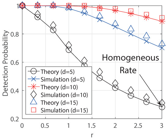
Figure 3. Theoretical and simulation result for Theorem 3.

In Figure 4, we obtain the error of parameter estimation for p with respect to the sampling cost K for the algorithm DPE(K). We consider the case $d=5$ and we set the error between true parameter p and estimated parameter $\widehat{p}$ by using the distance $|p - \widehat{p}|$. We plot the error for different values of p ($p=1,2,3,4$) by averaged values of 100 runnings of the algorithm. We use the step size $\delta =0.1$ and $p_{max}=5$. In the result, we see that the algorithm DPE(K) estimates the true parameter more accurately when p is large. This is because a large decaying parameter makes the snapshot more balanced from the source, and this enables to estimate the true parameter with less fluctuation.

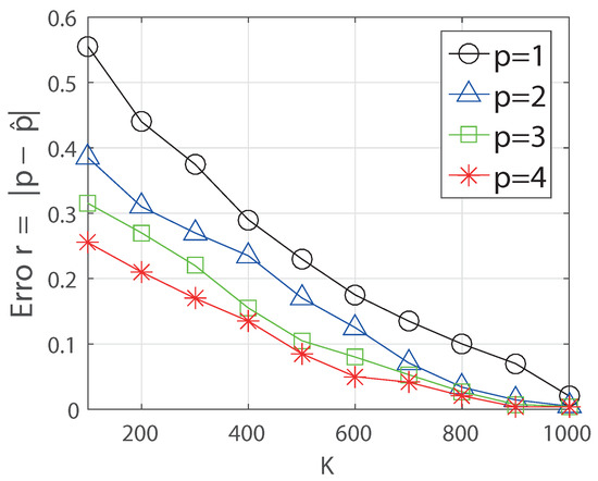
Figure 4. Simulation result for the estimation error $|p - \widehat{p}|$ with respect to the sampling cost K for the algorithm DPE(K). ($N=1000$.)

In Figure 5, we obtain the detection probabilities for degree $d=3$ with respect to decaying parameter p. In this simulation, we compare two results $\left(i\right)$ known parameter (true) $\left(ii\right)$ unknown parameter (estimated), respectively. The known parameter means that the true decaying parameter is given a prior, and we use it in the simulation. The unknown parameter means we do not know the true parameter so that we need to estimate it using the algorithm DPE(K) first. Then we obtain the detection probability. In the result, we check that the detection probability increases as p increases and the reduction of detection performance is not much even though we use the estimated parameter using DPE(K) for $K=500$.

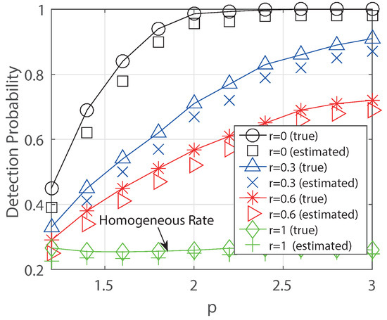
Figure 5. Detection probability by varying the parameter p for the 3-regular tree. We compare the results between true parameter p (true) and estimated parameter p (estimated) using the algorithm DPE(K). ($K=500$.)

6.2. Random Graphs

We consider Erdös-Rényi (ER), Scale-Free (SF) and Small World (SW) graphs. In the ER graph, we choose its parameter so that the average degree by 4 for 2000 nodes. In the SF and SW graphs, we choose the parameter so that the average ratio of edges to nodes by 1.5 for 2000 nodes. It is known that obtaining the MLE is hard for the graphs with cycles, which is ♯P-complete. Due to the reason, we first construct a diffusion tree from the Breadth-First Search (BFS) as used in [1]: Let ${\sigma }_v$ be the infection sequence of the BFS ordering of the nodes in the given graph, then we estimate the source $v_{\mathtt{bfs}}$ that solves the following:

$$\begin{array}{c}\hfill v_{\mathtt{bfs}}=arg{\displaystyle \underset{v\in G_N}{max}}\mathbb{P}({\sigma }_v|v)R(v,T_b\left(v\right)),\end{array}$$

(20)

where $T_b\left(v\right)$ is a BFS tree rooted at v and the information spreads along it. The BFS tree is a good approximation for our model because the decaying rates with the same distance to the source are same, and the nodes closer to the source have a higher diffusion rate. Then, we obtain the detection probabilities for each graph by increasing the parameter p as in Figure 6. We first simulate the case for true parameter i.e., it is given as a prior. Next, we also consider the parameter is hidden so that we need to estimate it. In this case, we replace the rumor centrality $R(v,G_N)$ for chosen node v by $R(v,T_b\left(v\right))$ in the algorithm DPE(K). As a result, we see that the detection probabilities increase as the parameter p increases and they decrease as the parameter r increases for three random graphs. We also see that if the decay level $r=p-1$, the detection probabilities are same as those of homogeneous diffusion rate. Further, we see that the detection is better on ER random graph than the other two networks because ER has symmetric locally tree structure, the decaying effect for large detection probability. Finally, for the unknown parameter p, we estimate the parameter using the algorithm DPE(K) with 100 iterations as in Table 1 and we check that the degradation of detection performance is not much even though we use the estimated parameter using DPE(K) if the sampling cost is sufficient.

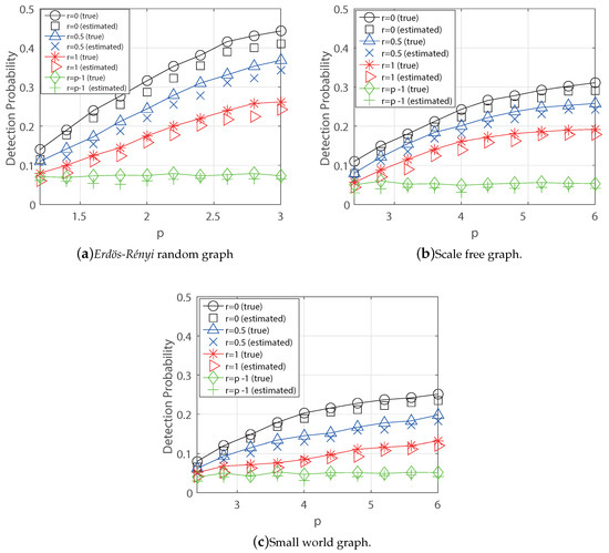
Figure 6. Detection Probabilities (true and estimated parameter) for Synthetic Graphs ((a) ER random graph, (b) Scale Free graph, and (c) Small World graph ($K=500$).

Table 1. Averaged value of estimations of parameter p using DPE(K) for general graphs ($K=500$). We use the step size $\delta =0.1$ and $p_{max}=10$.

True p	ER	SF	SW	PG	FB	WiKi
2	1.82	2.23	2.08	1.93	1.81	1.93
3	3.26	3.72	3.35	2.83	2.84	3.11
4	3.71	3.83	4.23	4.32	3.81	4.13
5	4.84	4.72	4.73	5.28	4.93	4.91
6	5.84	5.82	5.88	6.28	5.83	5.91

6.3. Real World Graphs

For the Facebook network in Figure 7b, we use the data in [21] where generates an undirected graph consisting of 4039 nodes and 88,234 edges. Each edge corresponds to a social relationship (called FriendList) and the diameter is 8 hops. The US power grid network Wiki consists of 4941 nodes and 6594 edges, and the diameter is 46 hops. For the WiKi-vote network, we use the data in [22] where generates 7115 nodes and 103,689 edges, and the diameter is 7 hops. In these networks, we also use the BFS approach in (20) to estimate the source and apply the BFS tree to estimate the parameter p in DPE(K) as in Table 1 with 100 iterations. Further, we see that the detection probabilities for the three networks increase as p increases and if the decal level $r=p-1,$ they become the results of homogeneous rate in Figure 7. We also see that the detection is better on the US power grid network than the other two networks because it has a large network diameter that gives more chances to detect the source using the diffusion snapshot.

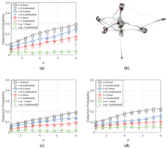
Figure 7. Detection Probabilities (true and estimated parameter) for Real-world Networks ((a) US power grid network, (b) Facebook Network [21], (c) Facebook network, and (d) Wiki-vote network ($K=500$).

7. Discussion

Our results show that decaying of information diffusion over distance from the source has a positive effect in most cases on inferring the source of information. In particular, the results show that if only mild conditions are satisfied, the source can be found as probability one no matter how much time passes for the regular tree structure. This is due to the fact that the spreading patterns which corresponding the decaying of information spreads more evenly with respect to the center of the infection graph. This phenomenon also occurs similarly with general graphs, making it easier to find the source.

The first limitation of this result is that the diffusion model under consideration does not cover the various decaying patterns due to some technical problem for analysis. For example, we can also consider the decaying by an exponential function such as ${\lambda }_h\left(p\right)=c{e}^{-ph}$ for some constant $c>0$ or by power-law function ${\lambda }_h\left(p\right)={\lambda }_0/h^p$, etc. However, we find some mathematical intractability to obtain analytical detection probability. As a second limitation, we did not consider the decaying with respect to time this is also because of hardness for tracking the infection time of diffusion.

As future work, we will consider more general decaying models that can be explainable of heavy-tail decaying and light-tail decaying patterns. We hope that this direction will give more chances to find some tractability for analysis of various decaying models. Further, we will obtain some analytical results for detecting the source of the Erdös-Rényi random graph because it is the simplest random graph.

8. Conclusions

In this paper, we consider an information source finding problem when the diffusion rate of information decays with respect to the distance from the source. We first show that the MLE is same as that of the homogeneous diffusion rate of information if the diffusion decays with respect to the distance from the source. We then obtain the closed form of detection probability of the MLE when the underlying graph is a regular tree for two exponential decaying models. Different to the prior result, the detection probability is larger than zero in the line graph and there is a non-neglectable improvement of detection for any degree of a regular tree. Next, we consider the case that the decaying model parameter is hidden for two decaying models above. To do that, we design a heuristic estimation algorithm for the true parameter by using the diffusion snapshot information, appropriately. Finally, we validate our theoretical result for the regular tree using the MLE and for over popular random graphs and real-world networks using the heuristic Breath-First-Search (BFS) estimator. We obtain that the detection probability can be above 80% for the regular tree, and it can be above 30% if the diffusion rate decays, whereas it is about 20% without decaying in the real-world graphs.

Appendix A.1. Proof of Lemma 2

Suppose that $N_1\left(t\right)$ has rate ${\lambda }_{m+k}\left(p\right)=\frac{{\lambda }_0}{p^{(m+k)}}$ and $N_2\left(t\right)$ has rate ${\lambda }_m\left(p\right)=\frac{{\lambda }_0}{p^m}$ at time t, respectively. Let $t+1$ be the embedding point of the next infection occur. Then, there are two possible events at time $t+1$, infection occurs in $N_1$ or $N_2$. By the exponential distributions, we obtain (13) by

$$\begin{array}{c}P\left(\mathrm{infection}\mathrm{occurs}\mathrm{in}{N}_1\mathrm{at}t+1\right)=\hfill \\ P(|N_1(t+1)-N_2(t+1)|=k+1)=\frac{{\lambda }_{m+k}\left(p\right)}{{\lambda }_{m+k}\left(p\right)+{\lambda }_m\left(p\right)}=\frac{\frac{{\lambda }_0}{p^{(m+k)}}}{\frac{{\lambda }_0}{p^{(m+k)}}+\frac{{\lambda }_0}{p^m}}=\frac{1}{1+p^k}.\hfill \end{array}$$

(A1)

One can easily obtain (14) by similar calculation and this completes the proof of Lemma 2.

Appendix A.2. Proof of Lemma 3

We will prove this by induction on k. First, consider the case $k=0,$ then we have

$$\begin{array}{cc}\hfill P\left(C^0\right)& =\frac{1}{1+p^{-1}}P\left(C^{-1}\right)+\frac{p}{1+p}P\left(C^1\right)=\frac{2p}{1+p}P\left(C^1\right),\hfill \end{array}$$

(A2)

and this implies that $P\left(C^1\right)=\frac{1+p}{2p}P\left(C^0\right).$ Next, If $k=1,$ we have $P\left(C^1\right)=\frac{1}{1+p^0}P\left(C^0\right)+\frac{p^2}{1+p^2}P\left(C^2\right)$ and $P\left(C^2\right)=\frac{1+p^2}{p^2}(\frac{1+p}{2p}P\left(C^0\right)-\frac{1}{2}P\left(C^0\right))=\frac{1+p^2}{2p^3}P\left(C^0\right).$ Using Equation (12) and induction hypothesis, we obtain

$$\begin{array}{c}\hfill P\left(C^k\right)=\frac{1}{2p^{\frac{k(k-1)}{2}}}\frac{1+p^k}{p^k}P\left(C^0\right)=\frac{1+p^k}{2p^{\frac{k(k+1)}{2}}}P\left(C^0\right).\end{array}$$

(A3)

By the symmetry $P\left(C^k\right)=P\left(C^{-k}\right)$, and the total sum $P\left(C^k\right)$ of all integer k should be one, we obtain

$$\begin{array}{cc}\hfill {\displaystyle \sum _{k=-\infty }^{k=\infty }}P\left(C^k\right)& =2{\displaystyle \sum _{k=1}^{k=\infty }}P\left(C^k\right)+P\left(C^0\right)=(2{\displaystyle \sum _{k=1}^{k=\infty }}\frac{1+p^k}{2p^{\frac{k(k+1)}{2}}}+1)P\left(C^0\right)=1\hfill \end{array}$$

(A4)

Now let $E\left(p\right)=2{\sum }_{k=1}^{k=\infty }\frac{1+p^k}{2p^{\frac{k(k+1)}{2}}}+1$ and then the bound of $P\left(C^0\right)=1/E\left(p\right)$ is determined by $E\left(p\right)$. Lemma 3 shows $P(C^0|even)=2/E\left(p\right)$ which leads to same conclusion on bound of $P\left(C^0\right)$. If $p\le 1$, $E\left(p\right)$ goes to infinity. It means $P\left(C^0\right)$ and $P\left(C^1\right)$ goes to 0 as time goes to infinity. If $p>1$, we have

$$\begin{array}{cc}\hfill E\left(p\right)& =2{\displaystyle \sum _{k=1}^{k=\infty }}\frac{1+p^k}{2p^{\frac{k(k+1)}{2}}}+1=2\left({\displaystyle \sum _{k=1}^{k=\infty }}\frac{1}{2p^{\frac{k(k+1)}{2}}}+{\displaystyle \sum _{k=1}^{k=\infty }}\frac{p^k}{2p^{\frac{k(k+1)}{2}}}\right)+1\hfill \\ \hfill & =2\left({\displaystyle \sum _{k=1}^{k=\infty }}\frac{1}{2p^{\frac{k(k+1)}{2}}}+{\displaystyle \sum _{k=1}^{k=\infty }}\frac{1}{2p^{\frac{k(k+1)}{2}}}+\frac{1}{2}\right)+1\hfill \\ \hfill & =2{\displaystyle \sum _{k=1}^{k=\infty }}\frac{1}{p^{\frac{k(k+1)}{2}}}+2.\hfill \end{array}$$

(A5)

Then, $E\left(p\right)$ has upper and lower bound $2<E\left(p\right)<\frac{2p}{p^2-1}+2$ because $0<2{\sum }_{k=1}^{k=\infty }\frac{1}{p^{\frac{k(k+1)}{2}}}<\frac{2p}{p^2-1}$ and this completes the proof of Lemma 3.

Appendix A.3. Proof of Lemma 4

We will prove this by induction hypothesis on $T_i\left(t\right)$ as follows. If $T_i\left(t\right)=1,$ $T_i\left(t\right)=u_i$ where $u_i$ have $d-1$ boundary edges and each edge has diffusion rate $\frac{{\lambda }_0}{d-1}$, we have $S_i\left(t\right)=(d-1)\frac{{\lambda }_0}{d-1}={\lambda }_0.$ If $T_i\left(t\right)=k\ge 2$, Let v be the last infected node in $T_i\left(t\right)$ and w be the infected node in $T_i\left(t\right)$ which spread rumor to v. Before infections of v, w’s boundary edges having rate ${\lambda }_{d\left(w\right)}\left(p\right)$ equally where $d\left(w\right)$ is the distance of node w from the source. Since v is one hop further from rumor source than $w,$ v’s boundary edges having rate $\frac{{\lambda }_{d\left(w\right)}\left(p\right)}{d-1}$ equally. When v is infected, one of w’s boundary edges is deleted from $E_i\left(t\right)$ and ($d-1$) edges of v are added to $E_i\left(t\right)$. Thus, the total sum of rate of $T_i\left(t\right)$ is same as that of $(T_i\left(t\right)\setminus v)$. Then, by the induction hypothesis, we have that of $(T_i\left(t\right)\setminus v)$ as $S_i={\lambda }_0$ and this completes the proof of Lemma 4.

Appendix A.4. Proof of Lemma 5

To prove this, we first denote $N\left(t\right)=N$ for the notational simplicity. Then, we use a mathematical induction on N i.e., the number of infected nodes in the graph. For $N=1,$ it is trivial because there is only one infected node which is the rumor source. Hence, for any diffusion rate, we have $P(T_i\left(t\right)>1/2|{\mathit{\lambda }}^1)=P(T_i\left(t\right)>1/2|{\mathit{\lambda }}^2)=0.$ Now, suppose this is true for $N-1$ and then define three events as

$$\begin{array}{c}\hfill \left\{\begin{array}{c}{A}_{1,s}:=\{T_i\left(t\right)>(N-1)/2|{\mathit{\lambda }}^s\},\hfill \\ A_{2,s}:=\{T_i\left(t\right)=(N-1)/2|{\mathit{\lambda }}^s\},\hfill \\ A_{3,s}:=\{T_i\left(t\right)<(N-1)/2|{\mathit{\lambda }}^s\},\hfill \end{array}\right.\end{array}$$

(A6)

where $s=1,2$. We let $B_s:=\{T_i(t+1)>N/2|{\mathit{\lambda }}^s\}$ then by the total probability law, we have

$$\begin{array}{cc}\hfill P\left(B_s\right)& ={\displaystyle \sum _i}P(B_s|A_{i,s})P\left(A_{i,s}\right)\stackrel{\left(a\right)}{=}\frac{1}{2}{\displaystyle \underset{N=odd}{\underbrace{\left(1·P\left(A_{1,s}\right)+P(B_s|A_{2,s})P\left(A_{2,s}\right)\right)}}}+\frac{1}{2}{\displaystyle \underset{N=even}{\underbrace{P(B_s|A_{1,s})P\left(A_{1,s}\right)}}}\hfill \\ \hfill & =\frac{1}{2}\left\{(1+P(B_s|A_{1,s}))P\left(A_{1,s}\right)+P(B_s|A_{2,s})P\left(A_{2,s}\right)\right\},\hfill \end{array}$$

(A7)

where the equality $\left(a\right)$ is from the fact that $P(N=odd)=P(N=even)=1/2$, $P(B_s|A_{3,s})=0$ for N is odd and $P\left(A_{2,s}\right)=P(B_s|A_{3,s})=0$ for N is even, respectively. From this result, it remains four terms in (A7) to obtain the result $P\left(B_1\right)\ge P\left(B_2\right).$ First, we see that $P\left(A_{1,1}\right)\ge P\left(A_{1,2}\right)$ from the induction hypothesis. Next, we will see that $P(B_s|A_{1,s})$ is also satisfied (This is the case that N is even). In this case, all the transition probabilities are one except the case that there are $N/2$ infected nodes in $T_i\left(t\right)$ and $(N-1)-N/2$ infected node in one of remained subtree. Let ${\beta }_s$ be the transition probability from this state to $N/2$ equally distributed for those two subtrees then one can check that ${\beta }_1\le {\beta }_2$ because

$$\begin{array}{cc}\hfill {\beta }_1=P({\displaystyle \underset{i}{min}}\{t_1,\dots ,t_d\}=t_2|{\mathit{\lambda }}^1)\stackrel{\left(a\right)}{=}& {\displaystyle \sum _{k=N/2}}\frac{{\lambda }_{\sigma (k-1)}^1}{{\lambda }_{\sigma \left(k\right)}^1+{\lambda }_{\sigma (k-1)}^1+{\sum }_{i=3}^d{\lambda }_1^1}={\displaystyle \sum _{k=N/2}}\frac{{\lambda }_{\sigma (k-1)}^1}{{\lambda }_{\sigma \left(k\right)}^1+{\lambda }_{\sigma (k-1)}^1+(d-2){\lambda }_1^1}\hfill \\ & \stackrel{\left(b\right)}{\le }{\displaystyle \sum _{k=N/2}}\frac{{\lambda }_{\sigma (k-1)}^2}{{\lambda }_{\sigma \left(k\right)}^2+{\lambda }_{\sigma \left(k\right)-1}^2+(d-2){\lambda }_1^2}={\beta }_2,\hfill \end{array}$$

(A8)

where $t_i$ be the random variable of the event that next infection occurs in the subtree $T_i$ when there are $N-1$ infected nodes in the graph. Here, ${\lambda }_{\sigma \left(k\right)}^i$ is the rate of this infection occurs in $T_1$ when there are k nodes. The equality $\left(a\right)$ is due to the exponential random variable of diffusion process and the inequality $\left(b\right)$ is from the fact that

$$\begin{array}{c}\hfill {\lambda }_{\sigma (k-1)}^1({\lambda }_{\sigma \left(k\right)}^1+{\lambda }_{\sigma (k-1)})\le {\lambda }_{\sigma (k-1)}^2({\lambda }_{\sigma \left(k\right)}^2+{\lambda }_{\sigma (k-1)}^2),\end{array}$$

(A9)

for all k since there are $d-2$ subtrees without any infections of ${\lambda }_i^1\ge {\lambda }_i^2$ for all $i\ge 1$. Then we have $P(B_1|A_{1,1})=1-{\beta }_1\ge 1-{\beta }_2=P(B_2|A_{1,2}).$ Next, we consider the probability $P(B_s|A_{2,s})P\left(A_{2,s}\right)$ (This is case that N is odd) and we first focus on $P(B_s|A_{2,s}).$ In this case, we have $P(B_1|A_{2,1})\ge P(B_2|A_{2,2})$ by the similar steps as before. Finally, we need to see that $P\left(A_{2,1}\right)\ge P\left(A_{2,2}\right).$ To show this is true for all $N\ge 1,$ we will show it holds for all $t>0$ as follows.

$$\begin{array}{cc}\hfill P\left(A_{2,1}\right)& ={\displaystyle \sum _{k_2+\cdots +k_d=(N-1)/2}}P((N-1)/2,k_2,\dots ,k_d|{\mathit{\lambda }}^1),\forall N,\hfill \\ \hfill & =P(T_1\left(t\right)={\displaystyle \sum _{i=2}^d}{T}_i\left(t\right)|{\mathit{\lambda }}^1)\hfill \\ \hfill & \stackrel{\left(a\right)}{=}P(T_1\left(t\right)=(d-1)T_2\left(t\right)|{\mathit{\lambda }}^1)\hfill \\ \hfill & \stackrel{\left(b\right)}{\ge }P(T_1\left(t\right)=(d-1)T_2\left(t\right)|{\mathit{\lambda }}^2)\hfill \\ \hfill & =P(T_1\left(t\right)={\displaystyle \sum _{i=2}^d}{T}_i\left(t\right)|{\mathit{\lambda }}^2)\hfill \\ \hfill & ={\displaystyle \sum _{k_2+\cdots +k_d=(N-1)/2}}P((N-1)/2,k_2,\dots ,k_d|{\mathit{\lambda }}^2)\hfill \\ \hfill & =P\left(A_{2,2}\right),\hfill \end{array}$$

(A10)

where the equality $\left(a\right)$ comes from the identical random process for all $T_i\left(t\right)$ and the inequality $\left(b\right)$ follows from the independence of random variables. Indeed, we see that

$$\begin{array}{cc}\hfill P(T_1\left(t\right)=(d-1)T_2\left(t\right)|{\mathit{\lambda }}^1)& ={\displaystyle \sum _{k=1}^{\infty }}P(T_1\left(t\right)=k|{\mathit{\lambda }}^1)P(T_2\left(t\right)=\frac{k}{d-1}|{\mathit{\lambda }}^1)\hfill \\ \hfill & \stackrel{\left(a\right)}{=}{\displaystyle \sum _{m=1}^{\infty }}P(T_1\left(t\right)=m(d-1)|{\mathit{\lambda }}^1)P(T_2\left(t\right)=m|{\mathit{\lambda }}^1)\hfill \\ \hfill & \stackrel{\left(b\right)}{\ge }{\displaystyle \sum _{m=1}^{\infty }}P(T_1\left(t\right)=m(d-1)|{\mathit{\lambda }}^2)P(T_2\left(t\right)=m|{\mathit{\lambda }}^2)\hfill \\ \hfill & =P(T_1\left(t\right)=(d-1)T_1\left(t\right)|{\mathit{\lambda }}^2),\hfill \end{array}$$

(A11)

where the equality $\left(a\right)$ follows from the fact that since $T_i\left(t\right)$ (In the tree, there is a unique path of any two nodes and the distribution of diffusion time from the rumor source to any node of distance $l>0$ follows hypo-exponential with rate $({\lambda }_1,\dots ,{\lambda }_l)$) takes integer values for all $t>0,$ the probability $P(T_2\left(t\right)=k/(d-1)|{\mathit{\lambda }}^1)$ is zero when k is not a multiple of $d-1.$ The inequality $\left(b\right)$ is from the fact that

$$\begin{array}{c}\hfill \frac{P(T_1\left(t\right)=m(d-1)|{\mathit{\lambda }}^1)}{P(T_2\left(t\right)=m|{\mathit{\lambda }}^2)}\ge \frac{P(T_1\left(t\right)=m(d-1)|{\mathit{\lambda }}^2)}{P(T_2\left(t\right)=m|{\mathit{\lambda }}^1)},\end{array}$$

(A12)

since the random process $T_1\left(t\right)$ and $T_2\left(t\right)$ have same distribution with exponential rates ${\lambda }_i^1\ge {\lambda }_i^2$ for all $i\ge 1$ of each edge. (We use the fact that $\frac{b}{a}\ge \frac{d}{c}$ if $b\ge d$ and $a\le c$, respectively. ) Next, we consider that

$$\begin{array}{cc}\hfill P\left(B_s\right)& =\frac{1}{2}\left\{(1+P(B_s|A_{1,s}))P\left(A_{1,s}\right)+P(B_s|A_{2,s})P\left(A_{2,s}\right)\right\}\hfill \\ \hfill & \ge \frac{1}{2}\left\{(2-\epsilon )P\left(A_{1,s}\right)+\epsilon P(B_s|A_{2,s})\right\}\hfill \\ \hfill & =P\left(A_{1,s}\right),asN\to \infty ,\hfill \end{array}$$

(A13)

for an arbitrary small number $\epsilon >0$ and consider that

$$\begin{array}{c}\hfill P(T_i\left(t\right)>N/2|{\mathit{\lambda }}^s)=\left\{\begin{array}{cc}P(T_i\left(t\right)>(N-1)/2|{\mathit{\lambda }}^s)\hfill & \mathrm{if}N=odd\hfill \\ P(T_i\left(t\right)>(N-1)/2|{\mathit{\lambda }}^s)\hfill \\ -P(T_i\left(t\right)=N/2|{\mathit{\lambda }}^s)\hfill & \mathrm{if}N=even,\hfill \end{array}\right.\end{array}$$

where $s=1,2.$ Then, from this relation and the fact that $P(N=odd)=P(N=even)=1/2,$ we have

$$\begin{array}{cc}\hfill P(T_i\left(t\right)>N/2|{\mathit{\lambda }}^1)& =\frac{1}{2}\left(2P(T_i\left(t\right)>(N-1)/2|{\mathit{\lambda }}^1)-P(T_i\left(t\right)=N/2|{\mathit{\lambda }}^1)\right)\hfill \\ \hfill & =P(T_i\left(t\right)>(N-1)/2|{\mathit{\lambda }}^1)-\frac{P(T_i\left(t\right)=N/2|{\mathit{\lambda }}^1)}{2}\hfill \\ \hfill & \stackrel{\left(a\right)}{\ge }P(T_i\left(t\right)>(N-1)/2|{\mathit{\lambda }}^2)-\frac{P(T_i\left(t\right)=N/2|{\mathit{\lambda }}^1)}{2}\hfill \\ \hfill & =P(T_i\left(t\right)>N/2|{\mathit{\lambda }}^2),\hfill \end{array}$$

(A14)

where $\left(a\right)$ is due to the induction hypothesis. Then, by using the fact that ${lim}_{N\to \infty }P(T_i\left(t\right)=N/2|{\mathit{\lambda }}^s)=0$ and the induction hypothesis, we have

$$\begin{array}{c}\hfill {\displaystyle \underset{N\to \infty }{lim}}P(T_i\left(t\right)>N/2|{\mathit{\lambda }}^1)\ge {\displaystyle \underset{N\to \infty }{lim}}P(T_i\left(t\right)>N/2|{\mathit{\lambda }}^2),\end{array}$$

and this completes the proof of Lemma 5.

References

- Shah, D.; Zaman, T. Detecting Sources of Computer Viruses in Networks: Theory and Experiment. In Proceedings of the ACM SIGMETRICS, New York, NY, USA, 14–18 June 2010. [Google Scholar]
- Shah, D.; Zaman, T. Rumor Centrality: A Universal Source Detector. In Proceedings of the ACM SIGMETRICS, London, UK, 11–15 June 2012. [Google Scholar]
- Shah, D.; Zaman, T. Rumors in a Network: Who’s the Culprit? IEEE Trans. Inf. Theory 2011, 57, 5163–5181. [Google Scholar] [CrossRef]
- Zhu, K.; Ying, L. Information Source Detection in the SIR Model: A Sample Path Based Approach. In Proceedings of the IEEE Information Theory and Applications Workshop (ITA), San Diego, CA, USA, 10–15 February 2013. [Google Scholar]
- Zhu, K.; Ying, L. A robust information source estimator with sparse observations. In Proceedings of the IEEE INFOCOM, Toronto, ON, Canada, 27 April–2 May 2014. [Google Scholar]
- Wang, Z.; Dong, W.; Zhang, W.; Tan, C.W. Rumor source detection with multiple observations: Fundamental limits and algorithms. In Proceedings of the ACM SIGMETRICS, Austin, TX, USA, 16–20 June 2014. [Google Scholar]
- Dong, W.; Zhang, W.; Tan, C.W. Rooting Out the Rumor Culprit from Suspects. In Proceedings of the IEEE International Symposium on Information Theory (ISIT), Istanbul, Turkey, 7–12 July 2013. [Google Scholar]
- Choi, J.; Shin, J.; Yi, Y. Information Source Localization with Protector Diffusion in Networks. IEEE/KICS J. Commun. Netw. 2017, 21, 136–147. [Google Scholar] [CrossRef]
- Choi, J.; Moon, S.; Woo, J.; Son, K.; Shin, J.; Yi, Y. Rumor Source Detection under Querying with Untruthful Answers. In Proceedings of the IEEE INFOCOM, 2017 IEEE Conference on Computer Communications, Atlanta, GA, USA, 1–4 May 2017. [Google Scholar]
- Choi, J.; Yi, Y. Necessary and Sufficient Budgets in Information Source Finding with Querying: Adaptivity Gap. In Proceedings of the 2018 IEEE International Symposium on Information Theory (ISIT), Vail, CO, USA, 17–22 June 2018. [Google Scholar]
- Ohsaka, N.; Yamaguchi, Y.; Kakimura, N.; Kwarabayashi, K. Maximizing Time-Decaying Influence in Social Networks. In Proceedings of the Joint European Conference on Machine Learning and Knowledge Discovery in Databases, Riva del Garda, Italy, 19–23 September 2016; pp. 132–147. [Google Scholar]
- Bubeck, S.; Devroye, L.; Lugosi, G. Finding Adam in random growing trees. Random Struct. Algorithms 2017, 50, 158–172. [Google Scholar] [CrossRef]
- Khim, J.; Loh, P.-O. Confidence Sets for Source of a Diffusion in Regular Trees. IEEE Trans. Netw. Sci. Eng. 2015, 4, 27–40. [Google Scholar] [CrossRef]
- Luo, W.; Tay, W.P.; Leng, M. How to Identify an Infection Source With Limited Observations. IEEE J. Sel. Top. Signal Process. 2014, 8, 586–597. [Google Scholar] [CrossRef]
- Prakash, B.A.; Vreeken, J.; Faloutsos, C. Efficiently Spotting the Starting Points of an Epidemic in a Large Graph. In Proceedings of the IEEE International Conference on Data Mining (ICDM), New Orleans, LA, USA, 18–21 November 2017. [Google Scholar]
- Zhu, K.; Chen, Z.; Ying, L. Catch’Em All: Locating Multiple Diffusion Sources in Networks with Partial Observations. In Proceedings of the AAAI, San Francisco, CA, USA, 4–9 February 2017. [Google Scholar]
- Ji, F.; Tay, W.P. An Algorithmic Framework for Estimating Rumor Sources With Different Start Times. IEEE Trans. Signal Process. 2017, 65, 2517–2530. [Google Scholar] [CrossRef]
- Fanti, G.; Kairouz, P.; Oh, S.; Viswanath, P. Spy vs. In Spy: Rumor Source Obfuscation. In Proceedings of the ACM SIGMETRICS, Portland, OR, USA, 15–19 June 2015. [Google Scholar]
- Luo, W.; Tay, W.P.; Leng, M. Infection Sprading and Source Identification: A Hide and Seek Game. IEEE Trans. Signal Process. 2016, 64, 4228–4243. [Google Scholar] [CrossRef]
- Fanti, G.; Viswanath, P. Anonymity Properties of the Bitcoin P2P Network. arXiv 2017, arXiv:1703.08761. [Google Scholar]
- Leskovec, J.; McAuley, J. Learning to discover social circles in ego networks. In Proceedings of the Neural Information Processing Systems (NIPS), Lake Tahoe, NV, USA, 3–8 December 2012. [Google Scholar]
- Leskovec, J.; Huttenlocher, D.; Kleinberg, J. Predicting Positive and Negative Links in Online Social Networks. In Proceedings of the 19th International Conference on World Wide Web, Raleigh, NC, USA, 26–30 April 2010. [Google Scholar]
© 2019 by the authors. Licensee MDPI, Basel, Switzerland. This article is an open access article distributed under the terms and conditions of the Creative Commons Attribution (CC BY) license (http://creativecommons.org/licenses/by/4.0/).