Fast Convolutional Neural Networks in Low Density FPGAs Using Zero-Skipping and Weight Pruning

Abstract

Edge devices are becoming smarter with the integration of machine learning methods, such as deep learning, and are therefore used in many application domains where decisions have to be made without human intervention. Deep learning and, in particular, convolutional neural networks (CNN) are more efficient than previous algorithms for several computer vision applications such as security and surveillance, where image and video analysis are required. This better efficiency comes with a cost of high computation and memory requirements. Hence, running CNNs in embedded computing devices is a challenge for both algorithm and hardware designers. New processing devices, dedicated system architectures and optimization of the networks have been researched to deal with these computation requirements. In this paper, we improve the inference execution times of CNNs in low density FPGAs (Field-Programmable Gate Arrays) using fixed-point arithmetic, zero-skipping and weight pruning. The developed architecture supports the execution of large CNNs in FPGA devices with reduced on-chip memory and computing resources. With the proposed architecture, it is possible to infer an image in AlexNet in 2.9 ms in a ZYNQ7020 and 1.0 ms in a ZYNQ7045 with less than 1% accuracy degradation. These results improve previous state-of-the-art architectures for CNN inference.

1. Introduction

Artificial intelligence associated with image classification [1] is largely used in computer vision applications improving computer vision tasks, such as image classification, object detection, and image segmentation. When used in edge devices, these methods and algorithms turn embedded devices into smart systems that can take decisions based on the smart analysis of collected data.

Deep neural networks (DNN) have attracted the attention in the field of artificial intelligence due to its abilities to achieve data classification accuracy close to that achieved by humans. A type of DNN used to classify images is the convolutional neural network (CNN) that identifies correlations among data inputs in order to classify them. For example, it can identify correlations between pixels of an image to identify the objects present in an image. Any DNN is made of a series of layers of connected neurons each with an associated weight similar to the neuron structure of a human brain. After being trained, the DNN can classify new data not seen during the training phase.

CNNs have a particular class of layers in the hidden layers known as convolutional. In these layers, a set of 3D convolutions are executed between groups of weights (3D kernels) and input maps produced by the previous layer to produce a set of output maps for the next layer. This large number of convolutions permits to discover features of the image. The final layers of a CNN are usually fully connected (FC), whose name derives from the fact that all nodes of a layer are connected to all nodes of the previous layer. The last fully connected layer outputs the result of the inference with each node corresponding to a class probability. Convolutional and fully connected layers are the main layers of a CNN.

The number and type of layers and kernels determines the accuracy of the network. The first CNNs were regular networks based on the main two layers described. The first well known CNN was LeNet [2] with a total of 60K weights distributed by five layers. The network was applied for digit classification with small images. A much larger CNN, AlexNet [3], was presented in the ImageNet Challenge for image classification, with five convolutional layers followed by three fully connected layers with a total of 61M weights and 724 MAC (Multiply-ACcumulate) operations to process images of size $224\times 224\times 3$ with a Top-5 error rate around 15 %. Another well known regular CNN model is VGG-16 [4] with 16 layers, $2.2\times$ more weights than AlexNet and 15.5 GMAC (Giga Multiply-ACcumulate) operations with a Top-5 error rate around 7%.

Other networks have followed, such as the GoogleNet [5], with a new type of layer: the inception module, consisting of parallel convolutions. GoogleNet is a deep CNN with 22 layers with a total of 6M weights and 1.46 GMACs to process a single image. Besides the inception layer, other modifications such as $1\times 1$ convolutions have improved the accuracy of GoogleNet when compared to previous models.

The first CNN exceeding human level accuracy was ResNet [6], which won the ImageNet Challenge in 2016 with 152 layers. ResNet introduced a new module that contains an identity connection to reduce the complexity of the training and, similar to GoogleNet, also uses $1\times 1$ convolutions. The model consists of 60M weights and a total of 11.3 GMACs.

Several other CNNs were proposed in the last years, some regular and some irregular with layers different from the usual convolutional and fully connected layers. Running any of these networks in an embedded system with strict performance, memory and energy constraints is a challenge because of the high number of weights and operations. Therefore, it is very important to find efficient methods and architectures to run large CNNs in low cost embedded platforms.

In this paper, a set of optimization techniques, namely fixed-point representation, zero-skipping, dynamic pruning and coarse weight pruning, are used to improve the inference execution time and reduce memory requirements of a state-of-the-art configurable architecture [7] designed for running CNN in low density FPGAs (Field-Programmable Gate Arrays) for smart embedded computing. The architecture supports the execution of large CNN in FPGA devices with small on-chip memory size and low resources. The baseline architecture considers the following optimizations:

• Fixed-point quantization: Activations and weights are represented with fixed-point format whose size can be different for each layer.
• An efficient method is used to calculate the convolutional layers that is independent of the size of the convolution window.
• Image batch: Convolutional layers are run for multiple images before running the fully connected layers.
• Convolutional and fully connected layers run with dedicated modules improving the implementation of each type of layer.

This paper improves the baseline architecture with the following techniques:

• Zero skipping in the convolutional layers where multiplication with zero valued activations are skipped;
• Dynamic zeroing of activations in convolutional layers; and
• Coarse pruning of fully connected layers where blocks of redundant weights are cut reducing the memory size required to store them and the number of operations.

The paper is organized as follows. Section 2 describes the related work on FPGA implementations of CNNs and optimization methods based on data reduction. Section 3 describes the fundamentals of convolutional neural networks. Section 4 describes the baseline architecture for CNN execution of large CNNs in low density FPGAs. Section 5 describes the architectural modifications of the baseline architecture to support the set of optimization techniques. Section 6 introduces a model of the proposed architecture to help in the design of a dedicated architecture for CNN inference. Section 7 describes the results obtained with the proposed architecture. Section 8 concludes the paper.

2. Related Work

Devices and platforms for smart embedded computing must have low energy consumption and be low cost. Therefore, high performance devices are in general not appropriate since they either have high energy consumption or low power efficiency and are relatively expensive. Embedded processors achieve only a few dozen GFLOPs (Giga FLoating-point Operations Per second) with low power efficiency insufficient for real-time or almost real-time processing of CNNs. GPUs (Graphics Processing Units) offer thousands of GFLOPs at the cost of high energy consumption not appropriate for embedded computing. Dedicated high-performance processors (e.g., Tensor Processing Unit, TPU) with dozens of TOPs (Tera Operations per second) and high energy efficiency have high energy consumption and are therefore inappropriate for edge computing. Thus, the options are embedded GPUs, FPGAs and dedicated hardware solutions with application specific integrated circuits (ASICs). Dedicated solutions are the most efficient but very limited in terms of configurability and thus unable to keep with the fast dynamic evolution of neural networks. FPGAs are less efficient but very hardware flexible and can be tailored for each particular neural network.

FPGAs run CNN inference with high performance efficiency, because they can be reconfigured to best implement each different CNN model. Depending on the FPGA family, hundreds or even thousands of GFLOPs were already obtained in the execution of a CNN inference. FPGA implementations of CNNs started with small networks [8,9] and/or considering only convolutional layers [10] and now full CNN implementations [11] and automatic tools for the generation of CNN accelerators [12] are available.

In [13,14], FPGA implementations of complete CNN models were proposed. The former uses an architecture similar to that proposed in [10]. These works consider a flexible architecture that can run any convolutional layer with different shapes and sizes of convolution windows. The problem of this architecture is that the performance efficiency varies with the window sizes of convolutions. To eliminate this performance variability with the window size, Suda et al. [14] implemented convolutions as matrix multiplications by rearranging the input maps of the layer. However, the solution introduces a large overhead associated with the memory accesses and execution times necessary to rearrange the input maps. This overhead was partially eliminated in [15] using an accelerator for matrix multiplication and dedicated units to convert the inputs maps into a matrix.

A different direction was followed in [16] that instead of a flexible structure to run any layer, the authors proposed a pipelined architecture with a layer in each pipeline level. The work achieves 445 GOPs (Giga OPerations per second) (data represented with fixed-point 8–16 bits) in a Virtex7 VX690T. The approach permits the optimization of the architecture for each layer but requires other techniques such as fused layers [17] to account for the extra memory required to store intermediate maps and weights. A mid-term solution was proposed by Shen et al. [18]. They mentioned the inefficiencies of a single module to run all convolutional layers, where for some layers there is an under utilization of processing elements. On the other side, they stressed that using one hardware module for each layer reduces the available on-chip memory for each layer, increases the complexity of external memory accesses and increases the control structure reducing the available resources for the datapath. Their proposal is to consider an accelerator with several execution modules, each running a subset of the layers. The proposal achieved $2\times$ speedup for SqueezeNet in a Virtex7 FPGA. The work by Gong et al. [19] also proposes a fully pipelined FPGA accelerator for CNNs with 16-bit quantization and a layer-fused technique. The architecture implemented in a small ZYNQ7020 FPGA has an acceptable performance of 80 GOPs, but the complexity of the process referred by Shen et al. [18] reduces the efficiency of the solution for small density FPGAs.

Recently, the authors started to focus on low density FPGAs for the implementation of CNNs. In [20], small CNNs were implemented in a ZYNQ XC7Z020 with an average performance of 13 GOPs with weights represented as 16 bit fixed-point data. The same FPGA was used to implemented bigger CNN models, such as VGG16, with data represented with 8 bits [21]. Their design flow—Angel-Eye—maps CNNs onto the FPGA including some optimizations. It has a parameterizable hardware module that is run-time reconfigured to run different layers. Data in layers are quantized with the best fixed-point scale and bit width, showing that 8-bits are enough for state-of-the-art networks. The architecture achieves performances of 84 GOPs with an energy efficiency $10\times$ better than NVIDIA TK1 and TX1. In [19], introduced above, the authors implemented a pipelined architecture with weight pruning in fully connected layers in a ZYNQ XC7Z020 with data represented with 16-bit fixed-point achieving 80 GOPs.

A few techniques have been proposed to improve the execution of CNNs. One of the first techniques was data size reduction where smaller and simpler representations are used for activations and weights. In [22], it is shown that dynamic fixed-point data representations with 8 bits guarantee accuracies close to those obtained with 32-bit floating point. The size of data can be fixed for all layers or optimized for each layer [23]. In [24], the trade-off between the network size and precision was studied. They concluded that a binarized neural network requires 2–11 times more operations and weights than a CNN with 8-bit fixed-point weights to achieve a comparable accuracy on MNIST. The big advantage of binarized neural networks is that they are faster. The work also proposes a framework to map a trained binarized neural network on FPGA. Each layer is computed with a dedicated module in a pipeline fashion. The work was used to implement a network to run CIFAR-10 in a ZYNQ FPGA with performances over 2 TOPs (Tera OPerations per second).

A mixed representation of data was proposed in [25]. Different data representations for different layers are exhaustively explored to find the best representation for the best accuracy. The approach reduces resources and energy consumption without compromising accuracy. Running VGG16 with mixed precision in a ZYNQ7045 FPGA achieves a performance of 316 GOPs, almost three times better than previous approaches with fixed data size for all layers. While most authors considered fixed-point arithmetic and reduced data size, in [26], a new floating-point representation (block floating-point) is used with 8 and 16 bit data widths. The new representation reduces the accuracy loss and improves arithmetic operations of floating-point data. The architecture running VGG16 in a Virtex 7 VX690T achieves a performance of 760 GOPs.

The Winograd algorithm [27] and the Fast Fourier Transform (FFT) have been applied in the design of CNN models [28] as methods that reduce arithmetic complexity. The FFT was also considered in [29] but the complexity reduction is small for small kernels. A two-dimensional Winograd algorithm was considered in [30] and applied to both convolutional and fully connected layers. The circuit was tested running AlexNet and VGG in a ZC706 board and achieved a performance of 201 GOPs for AlexNet and 680 GOPs for VGG16 with higher energy efficiency than a Titan X GPU. In [31], similar results were obtained with the application of Winograd and FFT to AlexNet, ResNet and YOLO. For example, the proposed architecture achieves 855 GOPs and 2480 GOPs running the convolutional layers of AlexNet and VGG16 respectively in a large ZU9EG FPGA.

Another class of optimizations is known as data reduction, which includes all techniques to reduce the number of weights and/or activations of the network model as a way to reduce the required memory and computation of the target platform. A first approach to data reduction was proposed in [32] where deep neural networks are compressed using pruning and Huffman coding. Pruning cuts connections between neurons and consequently reduces the number of weights of the network. The results show that pruning the fully connected layers of AlexNet by 91% has a negligible effect over the network accuracy. In [33], the pruning is adapted to the underlying hardware matching the pruning structure to the data-parallel hardware arithmetic unit. Blocks of nodes are removed iteratively until there is a reduction in accuracy. The method was tested with a microcontroller, a CPU and a GPU. The GPU implementation achieved a speed-up of 1.25% with a model reduction of 53%.

Pruning is typically not applied to convolutional layers since the percentage of weights in these layers is quite below the number of weights in fully connected layers. In convolutional layers, the bottleneck is the high number of computations. Therefore, a zero-skiping method was proposed in [34] that avoids multiplications by activations with value zero. The work has observed that the application of the ReLU function reduces many output activations to zero and so the number of multiply-accumulations of the next layer can be reduced. The same work also considered dynamic zeroing of activation outputs whenever the value is close to zero within a threshold. The problem of the proposed architecture is that it requires large on-chip memory and memory bandwidth, which is not adequate for low density devices, and only considers optimizations in convolutional layers. The work was implemented in ASIC technology. In [35], an architecture implemented in FPGA was proposed that dynamically skips computations with zeros similar to what is done in [34]. The authors kept a dense format to store the matrix requiring that all weights be loaded from memory, and target high density FPGAs. The NullHop architecture proposed in [36] also exploits the sparsity of convolutional feature maps, consequence of zero activations generated by the ReLU activation function. The architecture uses a particular sparse matrix compression scheme that reduces the required memory to store the feature maps and reduces the memory bandwidth requirements. The proposal does not explore intra-kernel parallelism since it accesses a single weight of a kernel at a time. With a working frequency of 60 MHz, the peak performance of the architecture is 128 GOPs with weights represented with 16-bit fixed-point. Running VGG16, the performance increases to 471 GOPs (the average sparsity for this network is 3.7). In [37], the sparsity achieved with weight pruning is also explored. The proposal considers one weight of each kernel at a time and applies kernel transformations to kernels with a window size different than $3\times 3$ to a series of kernels of size $3\times 3$. The architecture implemented in a ZYNQ ZCU102 running VGG16 with data represented with 16-bit fixed-point has a performance of 309 GOPs at 200 MHz.

Mixed fixed-point representation of activations and weights, zero-skipping, dynamic pruning of activations and weight pruning are all optimization techniques that reduce the number of operations and the number of weights in CNN. Most of these optimization schemes were only considered in large density FPGAs or as dedicated hardware in ASIC (Applications Specific Integrated Circuit). In this paper, an architectural solution able to integrate all these optimizations that can be implemented in low density FPGAs for embedded computing is proposed.

The architecture proposed in this paper efficiently integrates all these optimization methods, namely mixed fixed-point representation of activations and weights, zero-skipping, dynamic pruning and block pruning of fully connected layers in FPGA. As far as we know, this is the first proposal to integrate all these methods in a single architecture targeting low density FPGAs. Compared to a baseline architecture without optimizations and to previous works, the proposed architecture improves the inference performance of large networks up to $5.8\times$ in a low density FPGA.

3. Convolutional Neural Networks

Convolutional neural networks consist of a series of processing layers of different types. Each layer receives a set of input feature maps (IFM) from the previous layer and generates output feature maps (OFM) to the next layer. In regular CNN, there are convolutional, fully connected and pooling layers. Some works consider other type of layers in their CNNs. For example, GoogleNet [5] has the inception layer and He et al. [6] introduced a new layer that contains an identity connection to reduce the complexity of training. CNNs with specific layers are usually known as irregular CNNs.

The most computational intensive are the convolutional layers in which a set of 3D kernel are convoluted with the IFMs to generate the OFMs. In this paper, we refer to the nodes of the feature maps as activations.

Each convolution of a 3D kernel over the IFMs produce one OFM. Therefore, the number of output feature maps generated in a convolutional layer is the same as the number of kernels at that layer. Some convolutional layers are followed by pooling layers that sub-sample the OFMs by merging neighbor activations into a single one using a max or average function.

The set of convolutional layers may be followed by one or more fully connected (FC) layers. A node in a fully connected layer is connected to all nodes of the previous layer. The last FC layer outputs the probabilities of each class of objects with one node for each class. These layers contain most of the weights of a CNN which must be stored and transferred from external memory to on-chip memory. Hence, they are very demanding in terms of memory space and memory bandwidth. In addition, while in the convolutional layers the same kernel is used many times, in a FC layer each kernel is used only once.

In all layers, each output is followed by an activation function. Several functions exist but recently the Rectified Linear Unit (ReLU) function is commonly used for its simplicity and good results. This function keeps the positive activations unaltered and zeroes the negative ones. Recently, some variations of this function have appeared, such as leaky ReLU, parametric ReLU, concatenated ReLU, and ReLU-6, that improve the training process.

Knowing that convolutional layers are computation intensive and that FC layers are memory bandwidth intensive, several optimization techniques apply to both types of layers while others are more appropriate to only one type of layer.

The most used optimization techniques to reduce the computational complexity, the required memory bandwidth and memory size are using fixed-point computation instead of floating-point and reducing the bit width of weights and activations. These techniques are known as data quantization. Fixed-point format uses a set of the bits to represent the integer part of the number and the remaining bits are used for the fractional part. The Q notation explicitly indicates this subdivision (e.g., Q3.5 means 3 bits for integer and 5 bits for fractional). Fixed-point numbers are also represented as an integer number plus a scale factor that determines the binary point position. Thus, for example, Q3.5 would have a scale factor of $2^{-5}$. Quantization of a CNN consists in determining the fixed-point format of activations and weights for each layer. When the fixed-point size is the same for all layers, the quantization only changes the scale factor for each layer. When different sizes are used for different layers, both the size and the scale factor must be determined.

Another technique to reduce the computational complexity is zero-skipping. The ReLU function converts negative values to zero and consequently many output activations are zero. Multiplying a weight by zero is useless so the zero-skipping technique does not run these multiplications reducing the processing time. In [34], the authors showed that for several known networks an average of up to 50% of input activations are zero. The number of zeros can be increased by applying dynamic pruning to the convolutional layers that sets activation to zero if their values are below a threshold. The same work has shown that within certain thresholds it is possible to dynamically prune activations without affecting the network accuracy.

Static pruning is also used as an optimization technique to reduce the number of weights. During training, weights below a certain threshold are cut. The technique is normally applied to the fully connected layers where the number of weights is very high and cut percentages of up to 90% can be used without affecting the network accuracy. Another frequently used optimization technique that reduces the impact of high memory transfer times of weights in the FC layers is the image batch. In this technique, several outputs of the last convolutional layer are calculated and batched before running the FC layers. This way, the weights of FC layers read from memory are then used for a batch of input maps amortizing the transfer time.

This paper proposes a very efficient architecture that considers zero-skipping, dynamic pruning, block pruning, fixed-point representations and image batch to be implemented in low density FPGAs for smart embedded systems. The integration of all these techniques in a single architecture permits the design of large CNNs in low density FPGAs with very high performance.

4. Baseline Architecture for CNN Inference

The architectural optimizations proposed in this paper are applied to a baseline architecture that implements large CNNs in low density FPGAs considering only 8-bit fixed-point representation format following the ideas of omi [7]. This architecture is designated as baseline architecture to be described in this section.

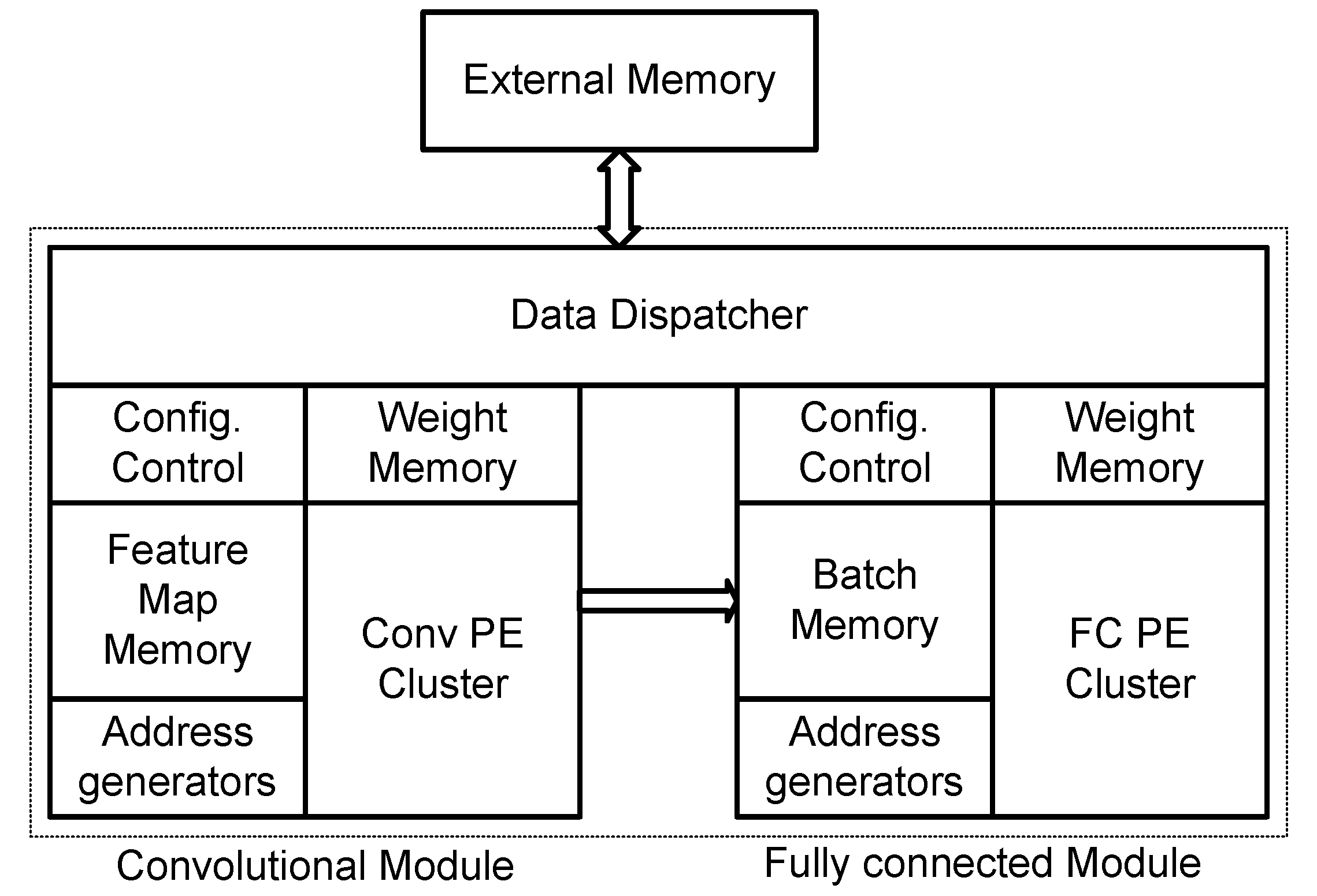
The baseline architecture was designed to allow the execution of large CNNs in low density FPGAs, that is, with low memory and computational resources. It has two main modules executing in parallel, one dedicated to convolutional layers and another to fully connected layers, as shown in Figure 1. This separation allows different optimization techniques to be applied independently to convolutional and fully connected layers.

Each module executes one layer at a time. Since each layer may have a particular number of maps and kernels, the modules have a set of configurable registers to set them for each specific layer. Thus, before executing a particular layer, the module is configured with the specific characteristics of the layer, namely number of kernels, size of kernels, source and destination addresses of activations and kernels, the existence of a pooling layer and fixed-point format.

The input image and the intermediate feature maps are stored in on-chip memory to be processed. If the on-chip memory is not enough, the image or the IFM is divided and processed in pieces. The output feature maps are stored in external memory and then reloaded for the next layer. This feature of the architecture permits the execution of larger CNNs in FPGAs with scarce on-chip memory resources.

The convolutions of convolutional layers and dot-products of fully connected layers are all done by clusters of processing elements (PE) that explore several levels of parallelism and have local memory to store kernels of weights. Pooling and activation function run in a central module shared by all PEs.

Running a CNN in the architecture works as follows:

• Each module is configured according to the layer features.
• The image or the input feature maps are loaded to the on-chip memory.
• Kernels are loaded into the local memories of the PE cluster.
• PE clusters execute the convolutions and dot-products.
• The results are sent to the pooling and activation module.
• The new activations are stored in external memory.
• Go to Step 3 if more kernels need to be loaded.
• The whole process repeats for each layer.

The configuration of the main modules and of the data dispatcher is executed by a processor. The processor configures the architecture according to the features of the layers to be executed and configures the direct memory access (DMA) blocks of the data dispatcher to read the feature maps and the kernels from external memory and write the feature maps back to external memory.

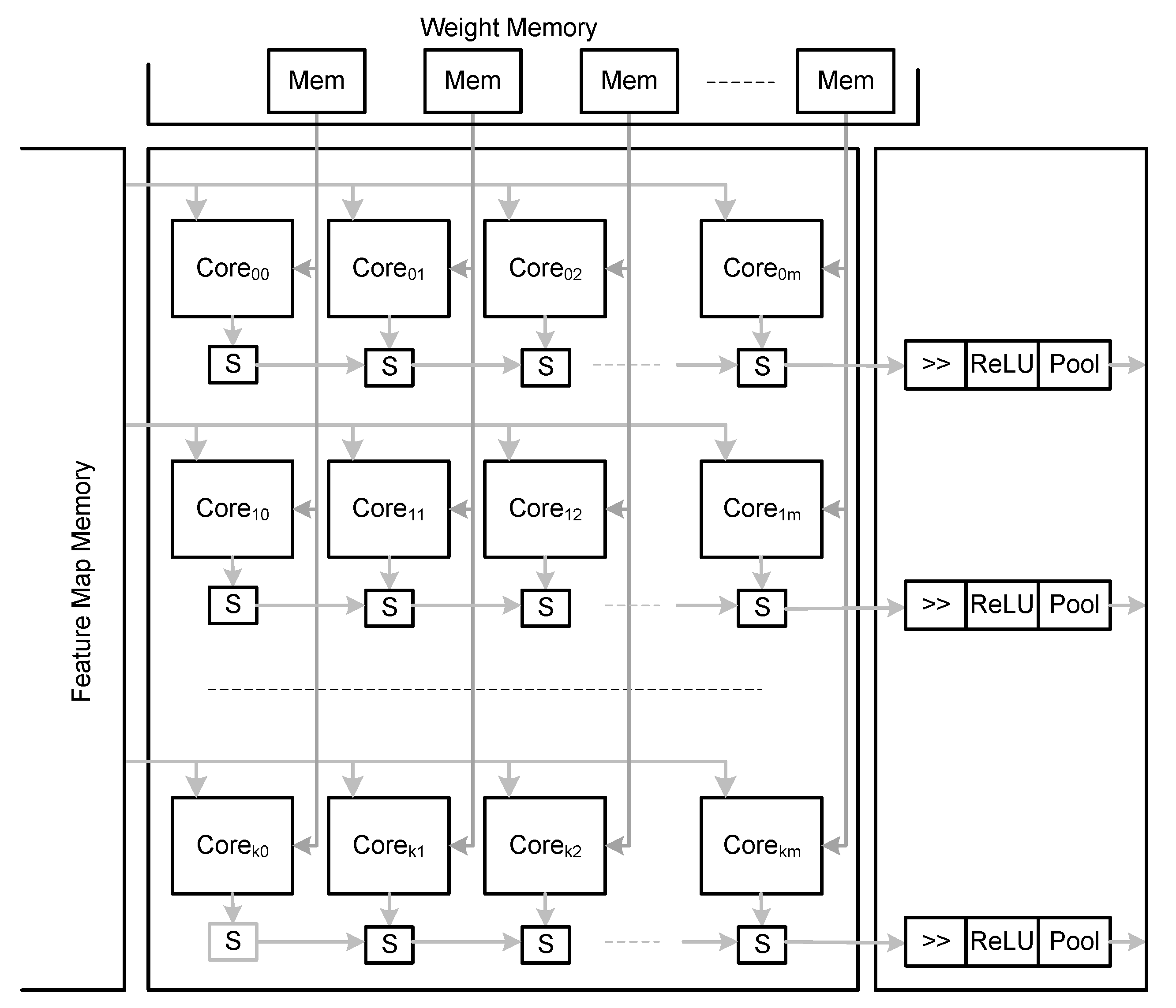
4.1. PE Clusters

The PE cluster for convolutions consists of a matrix of cores, as illustrated in Figure 2.

Cores of a column share a local memory used to store weights. The weights stored in the local memory are broadcasted to all cores of the column. A line of cores shares the same port of the feature map memory. Activations read from a port of the feature map memory are broadcasted to the cores of the line. The number of cores per line equals the number of kernels processed in parallel and the number of cores per column equals the number of ports of the feature map memory. The baseline architecture is statically configurable in the number of cores per line and per column.

Since all cores of a column receive the same kernel, they all contribute to the calculation of a single OFM (intra-output parallelism). Cores in the same line receive different kernels and therefore each produces a different OFM. The more cores there are in a line the more OFM are generated in parallel (inter-output parallelism).

The PE cluster of fully connected layers has the same structure of the cluster for convolutions but the number of lines of cores in the cluster is now determined by the batch size. In the fully connected layers the kernels have the same size of the IFM, which is the same as having a single IFM. Each kernel is applied to the whole IFM and produces a single activation. The intra-output parallelism is explored only when batch of OFM of the last convolutional layer is considered. Several OFM of the last convolutional layer can be stored before running the first fully connected layer. In this case, the same kernel can be reused for several batched OFM reducing the memory bandwidth requirements at the cost of some more on-chip memory to accumulate OFM.

Any core calculates dot products between activations and weights with a multiply-accumulate unit. MAC units are implemented for fixed-point activations and weights. Multiplication results are accumulated in the MAC units without bit loss. The final accumulation is sent to the central unit to be shifted according to the fixed-point scale factor of the layer, and truncated and pooled when the layer is followed by a pooling layer.

To explore dot-product parallelism, the core implements parallel MAC units to process multiple multiplications between activations and weights read in a single memory access. The baseline architecture considers 8-bit fixed-point data and 64-bit memory accesses. Therefore, each core processes and accumulates eight multiplications in parallel.

4.2. Feature Map Memory

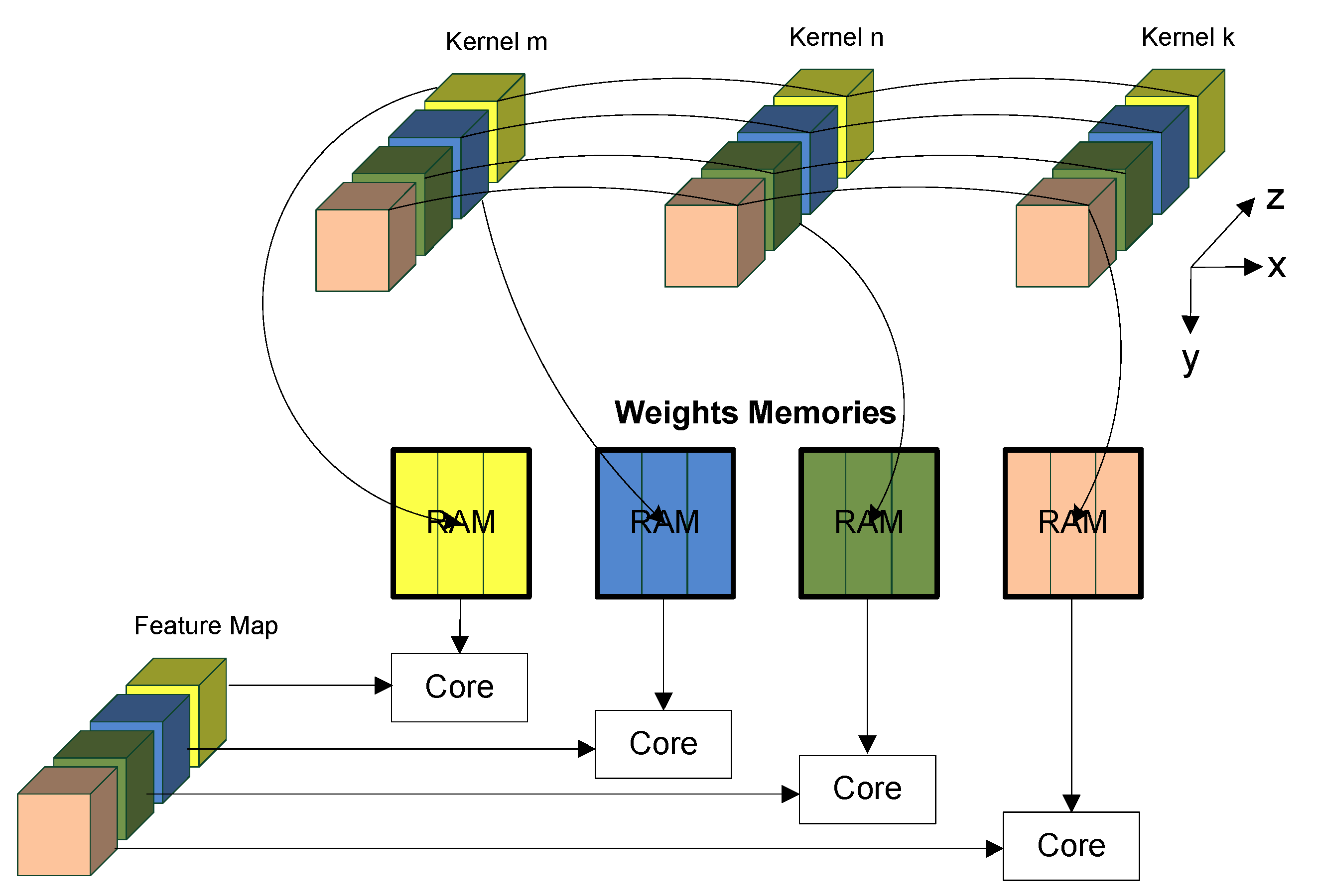
A major optimization feature of the baseline architecture is how convolutions are calculated. To be independent of the convolution window size and take advantage of kernel parallelism, the architecture considers 3D convolutions with activations and weights read as long vectors and multiply-accumulated in a long dot-product.

Each activation of an output feature is obtained from the dot product between a 3D kernel $x_k\times y_k\times z_k$ and the corresponding activations of the IFM of size $x_p\times y_p\times z_p$, where $z_p$ is the number of IFMs (see Figure 3).

As can be observed in Figure 3, both kernel and activations are read along the z-axis, followed by dimension x and then y. The weights of the kernel are all read sequentially from the memories of weights since they are stored in this order. The activations are read in sequence from the FMM (Feature Map Memory) but after $x_k\times z_k$ activations it has to jump to the next $y_k$ adding an offset to the address of the input feature memory being read. For a layer without stride or followed by pooling, the offset is $x_p\times z_p$. Formally, the dot product to calculate each step of the convolution is given by Equation (1).

$$D{P}_{conv}=\sum _{i=0}^{i=y_k-1}\sum _{j=0}^{j=x_k{z}_k-1}{W}_{i{x}_k{z}_k+j}\times P_{startAddr+i{x}_p{z}_p+j}$$

(1)

where startAddr is the address of the first activation of the block of the input feature map being convoluted. This operation is used to convolute a kernel with the set of input feature maps sliding the 3D kernel along the feature maps. If a layer is followed by a pooling layer, the output activations of the pooling window are pooled and only the pooling result is stored in the FMM. The advantage of the proposed method is that it keeps the performance efficiency of the 3D convolution independent of the size of the convolution window. Previous solutions required some kind of padding or filter serialization.

Considering a 3D input feature map of size $x_p\times y_p\times z_p$, a kernel of size $x_k\times y_k\times z_k$, a pooling window of size $x_{pool}\times y_{pool}$ and a stride of size s, the convolution of a kernel, $kl$, with the 3D input feature map is given by Algorithm 1.

Algorithm 1: Convolution with a 3D kernel.

$poolFunction$ is the function to be used in the pooling operation, such as maximum or average. The $startAddr$ function specifies the initial address of the feature memory map block to be convoluted with the 3D kernel. It depends on the size of the input feature map, the pooling size and the stride value. Given the first memory address where the feature map is stored, $initialAddr$, the $startAddr$ function is given by:

$$startAddr=initialAddr+k\times z_p+l\times z_p\times x_p+m\times z_p\times s+r\times z_p\times x_p\times s$$

The $startAddr$ function is generated by the address generators associated with the feature map memory.

Sending and receiving activations to and from the fully connected layers is simpler since there are no convolutions, only a long dot-product. Data from the batch memory are read and written only once for each kernel. When there is IFM batching, the batch memory consists of several separated memories, one for each map batch. The read and write addresses are common for all memories. The output activations from the cores are also shifted and truncated, such as in the convolutional layers, before being written back to memory. Batch memories are dual port to allow reading from the fully connected cores and writing of the next map batches.

5. Improved Architecture for CNN Inference

The baseline architecture was modified to support zero-skipping and dynamic pruning of activations in the convolutional layers and weight pruning in the fully connected layers.

5.1. Zero-Skipping and Dynamic Pruning of Activations

The baseline architecture reads several blocks of activations and multiplies them with the weights of kernels. If some of these activations are zero, then we have multiplications by zero. To avoid them, only non-zero activations should be considered.

The first consideration is to decide how the feature maps are stored. Two different cases may be considered: one that stores the complete feature map, including zeros, and then only the non-zero activations are considered for calculation and one in which only the non-zero activations are stored. Considering that the sparsity of a feature map is not too high (50% on average for known networks), storing only the non-zero elements requires extra index information, which for low sparsity is a high overhead. Besides, in this case, determining the correct indexes to read the activations according to the behavior of the send/receive activations module of the feature map memory is a complex task. Therefore, the first option was adopted, that is, we store the whole map, including zeros. For those networks with a high sparsity, storing compressed feature maps brings advantages about memory storage and bandwidth requirements. How to adapt the proposed architecture for these cases is out of scope of this paper and is left for future work.

When we read a block of activations, some of them may be zero. Thus, we cannot send the whole block to be multiplied by a block of weights as in the baseline architecture. For each non-zero activation, the correspondent weight is read from the weights memory and multiplied. In the baseline architecture, each local memory stores one kernel of weights and, therefore, since a specific weight must be read for each non-zero activation, it is not possible to explore dot-product parallelism with this structure. However, if we partition the kernel and the activations by multiple memories, then we can explore dot-product parallelism since several weights of a single kernel can be multiplied by activations in parallel (see Figure 4).

Instead of storing the whole kernel in a single memory, which only permits reading one weight at a time, kernels can be partitioned and stored in separate memories. The same partition is applied to the memory of activations so that multiple activations can be read in parallel.

Inter-output parallelism is applied by storing several different kernels in the same memory, that is, each memory position contains weights with the same index from different kernels. Hence, each activation is multiplied by weights of different kernels contributing to different dot-products, that is, to different output feature maps. The proposed optimized architecture also considers intra-output parallelism, where multiple activations of a single output feature map are generated in parallel. The partition of the feature map memory follows the same structure of the baseline architecture. However, while, in the baseline architecture the weights memory is the same for all cores in a column, in the optimized architecture, it cannot share the kernels among cores in the same column since activations from different ports of the feature map memory may have different indexes and, therefore, require access to different weights of the kernel. The weights memory must have multiple ports, one for each port of the feature map memory. Since the FPGA memories only have at most two parallel ports, data have to be replicated using more memories.

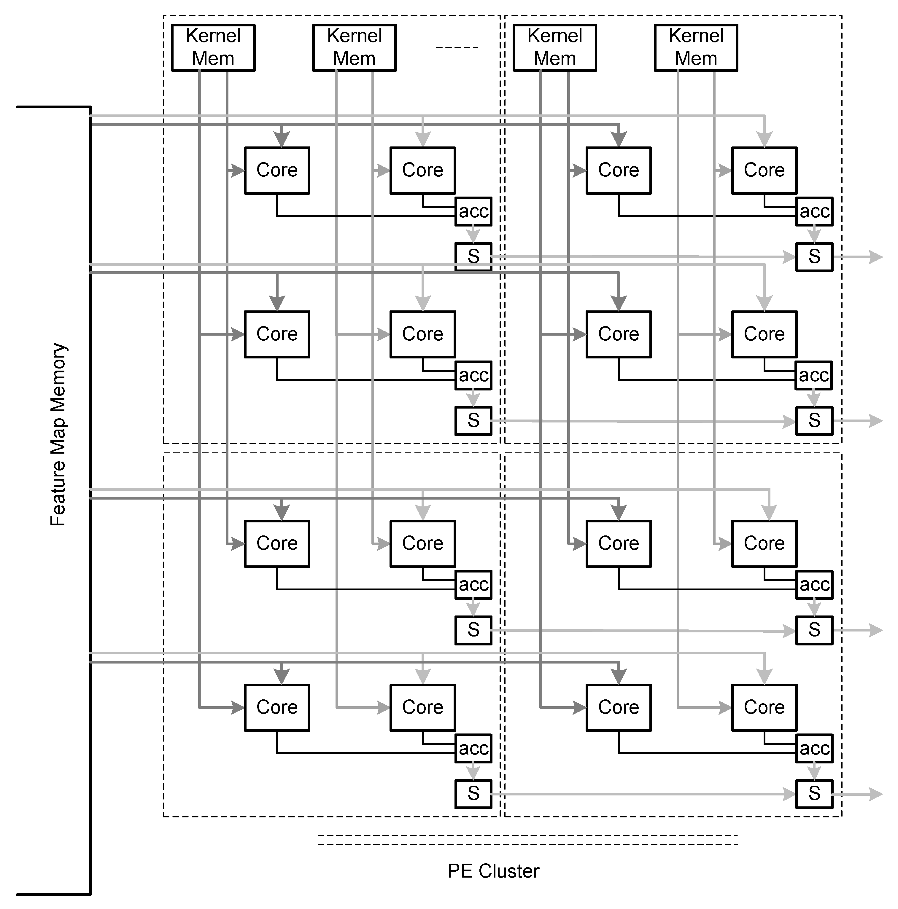
The structure of the PE cluster for the convolutional layers now has a slightly different structure compared to the cluster of the baseline architecture (see Figure 5).

The output of cores belonging to the same kernel are accumulated. In the configuration illustrated in Figure 5, kernels are partitioned into two memories but more partitions can be considered to expose more parallelism. Dual port weight memories feed data to two lines of cores that are connected to two ports of the feature map memory. The structure is scalable and can be replicated to include more cores to process the same kernels, different kernels and different ports of the feature map memory.

As stated above, to increase the intra-output parallelism, the kernels have to be replicated and consequently more on-chip memory is necessary. To reduce this memory requirement, local memories used to store the weights can operate at higher frequencies to feed more cores. Therefore, we considered another implementation of the architecture where the operating frequency of local memories is twice the frequency of the cores. With this dual-rate operation, a single dual-rate dual-port memory can feed four cores in a single cycle at the frequency of the cores (see Figure 6).

With more on-chip memories and memory bandwidth available, it is possible to increase the number of cores of the cluster, as long as there are resources available. The operating frequency of the cores may have to be reduced compared to their operating frequency in the baseline architecture, to guarantee half of the operating frequency of the on-chip memories.

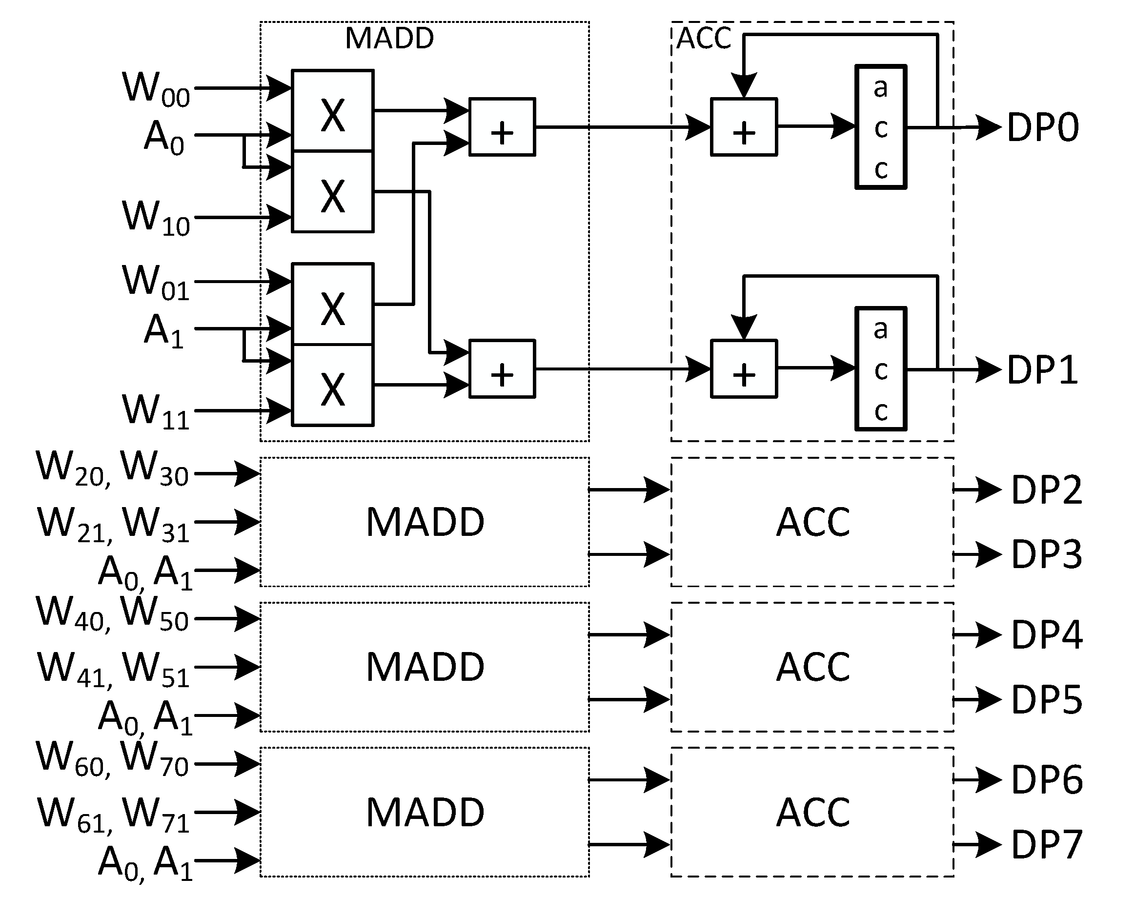
Each core in the zero-skipping architecture implements n parallel dot-products, where n is the number of partial kernels stored in each weight memory. An implementation of the core with n = 8 is illustrated in Figure 7).

The diagram in the figure illustrates the core considering a dot product parallelism of two. In this case, eight dot products, $D{P}_0..D{P}_7$, are calculated between a vector of two activations $A=[A_0,A_1]$, and eight vectors of two weights each, $W0=[W_{00},W_{01}]$, $W1=[W_{10},W_{11}]$, $W2=[W_{20},W_{21}]$, $W3=[W_{30},W_{31}]$, $W4=[W_{40},W_{41}]$, $W5=[W_{50},W_{51}]$, $W6=[W_{60},W_{61}]$, $W7=[W_{70},W_{71}]$.

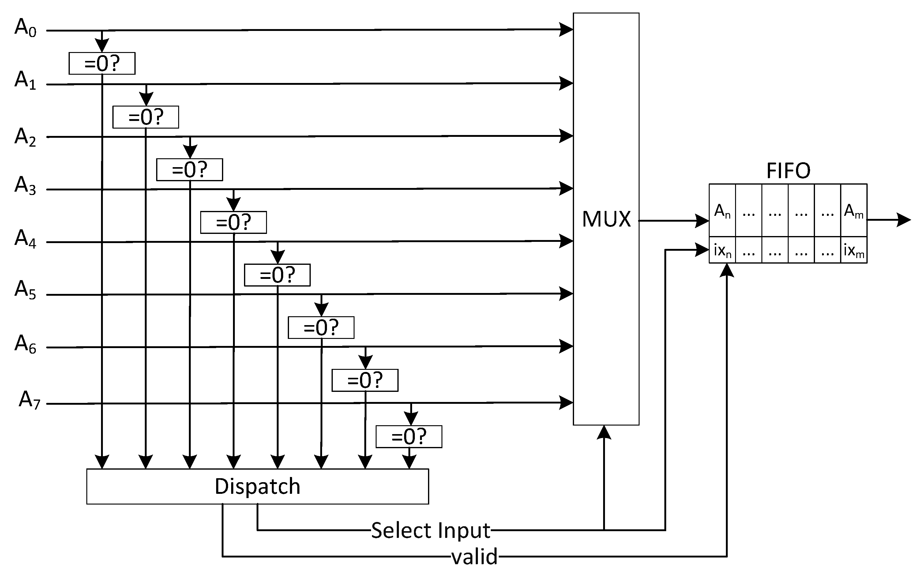
The reading process of activations in the zero-skipping architecture is similar to the one used in the baseline, except that activations must be dispatched in series. In the baseline architecture, a block of eight activations is read from the feature map memory and sent in parallel to the cores to be processed with the weights. In the zero-skipping architecture, each core processes only one activation at a time. Thus, the module still reads eight activations in a clock cycle but then only sends one non-zero activation per cycle. Zero activations are discarded (see Figure 8).

The circuit receives the eight activations, detects zero activations and then sends non-zero activations to the output FIFO together with an index relative to the activation position in the vector of eight activations.

A final modification of the convolutional cluster has to do with the dynamic pruning of activations. The pruning is made by the same module responsible for fixed-point scaling, activation function and pooling. All activations received from the PE cluster are compared to a fixed threshold. If it is lower than the threshold, the activation is zeroed.

5.2. Pruning of Weights in Fully Connected Layers

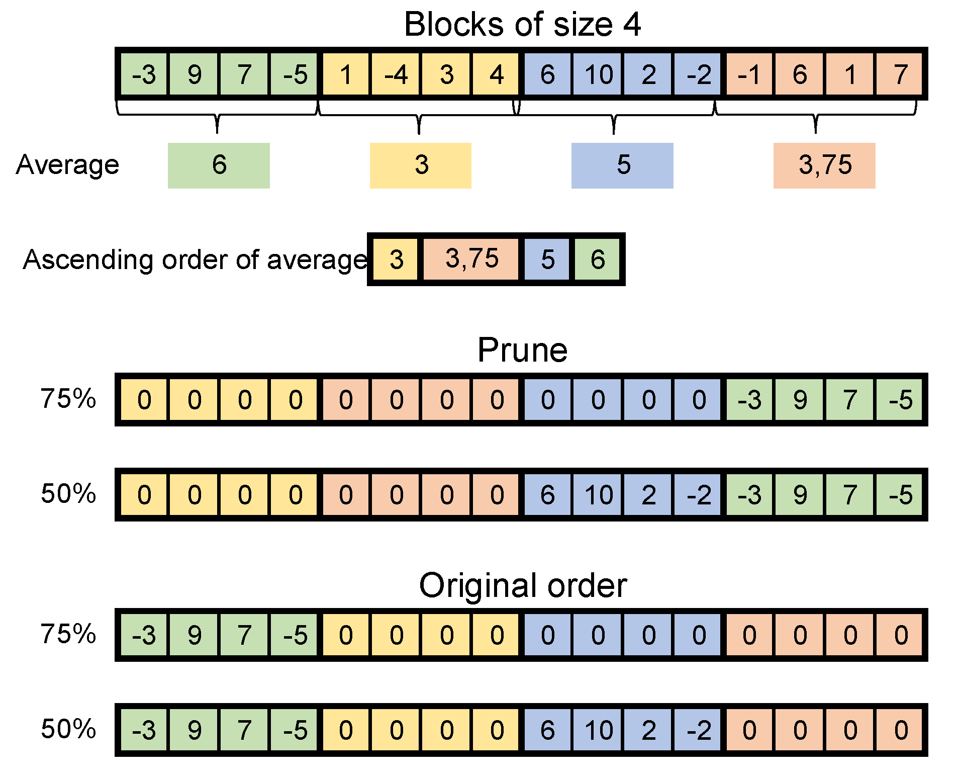
Pruning of weights reduces the required memory to store kernels but introduces sparsity in the kernels of weights and an overhead associated with the index information of the sparse vector of weights. The pruning reported in the literature (see, for example, [32]) in some layers are over 90%, which introduces a large sparsity in the kernel. To improve the hardware implementation and the performance of pruned networks, we adopt the block pruning technique, which performs a coarse pruning with blocks of weights. The method reduces the index overhead data and permits to efficiently use the parallel MACs of the processing units.

The technique prunes blocks of weights (similar to what is done in [33]) instead of single weights (see example in Figure 9).

The method determines the average magnitude of a block of weights, sorts them and then the blocks with the lowest average magnitude are pruned limited by a pruned percentage. The remaining blocks are stored as a sparse vector where each position contains the block of weights and the index of the next block.

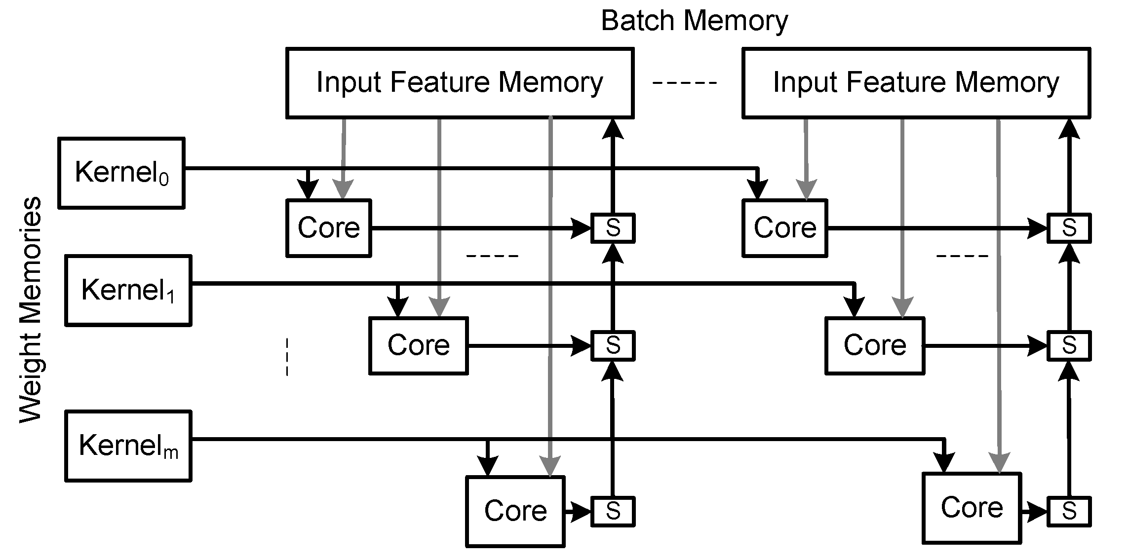
Considering this technique, the fully connected cluster has one local memory for each sparse kernel of weights and one local memory for each feature map instance (see Figure 10).

Each kernel memory requires one port from the input feature memory. Considering memories with at most two independent ports, the input feature memory must be replicated to supply activations to more than two kernel memories. The implementation of batch only requires one input feature memory for each batch since the kernels are shared by all batches. The cores are identical to those used in the baseline architecture.

6. Designing with the Proposed Architecture for Best Performance

The convolutional and the fully connected clusters work in parallel in a pipelined fashion. To obtain the best throughput, the delays of both PE clusters should be as close as possible. The execution times of the clusters depend on the number of cores, which depends on the available hardware resources, and the external memory bandwidth. In the following sections, we describe a performance and an area model of the architecture that helps the designer obtaining the architecture for best performance.

6.1. Performance Model

The execution time of the complete CNN, $Texe{c}_{CNN}$, is the sum of the execution time of convolutional layers, $Texe{c}_{CL}$, fully connected layers, $Texe{c}_{FCL}$, and the time to load the image to be inferred, $Tcom{m}_{image}$,

$$Texe{c}_{CNN}=Tcom{m}_{image}+\sum _{i=1}^{i=CL}Texe{c}_{C{L}_i}+\sum _{i=1}^{i=FCL}Texe{c}_{FC{L}_i}$$

(2)

where $CL$ is the number of convolutional layers and $FCL$ is the number of fully connected layers.

The execution throughput, $Th{r}_{CNN}$, of the architecture is given by

$$Th{r}_{CNN}=\frac{1}{max(Tcom{m}_{image}+{\sum }_{i=1}^{i=CL}Texe{c}_{C{L}_i},\frac{{\sum }_{i=1}^{i=FCL}Texe{c}_{FC{L}_i}}{batchSize})}$$

(3)

The batch size equals the number of cores in a column, $FCcoreC$, of the FC cluster. This throughput is in fact an average throughput since the batch technique generates $FCcoreC$ results for each execution of the FC layers.

The time to read the image from external memory depends on the image size, $imag{e}_{size}$ (bytes), and the memory bandwidth to external memory allocated to the convolutional module, $B{W}_{CL}$ (bytes/s), as follows:

$$\begin{array}{c}\hfill Tcom{m}_{image}=\frac{imag{e}_{size}}{B{W}_{CL}}\end{array}$$

(4)

The time to execute a convolutional layer depends on the time to load the input feature maps and the kernels and the time to execute the convolutions.

The time to load data from external memory depends on the size of the input feature maps, $IF{M}_{size}$, the number of 3D kernels, $nKernel$, the size of the 3D kernel, $kerne{l}_{size}$, and the external memory bandwidth. The size of the image and feature maps determines the number of times the kernels have to be reloaded. As stated above in the description of the baseline architecture, if any of these do not fit in the feature map memory the inputs have to be partitioned and processed separately. Therefore, the weights have to be read from external memory as many times as the number of image or IFM partitions.

To reduce the time to load the input data of the layer, layer computation and kernel loading can overlap, that is, while a set of kernels is being process, the next set of kernels can be loaded, as long as the local memories of the PE clusters are large enough to hold two kernels. In addition, the output activations are written to external memory during the layer execution.

Considering these aspects, the time to load all data associated with a convolutional, $dCommCL$, layer is given by:

$$\begin{array}{cc}\hfill dCommCL=\frac{IF{M}_{size}+\frac{IF{M}_{size}}{FM{M}_{size}}\times (nKernelP\times kerne{l}_{size})}{B{W}_{CL}}& \mathrm{with}\mathrm{overlap}\hfill \end{array}$$

(5)

$$\begin{array}{cc}\hfill dCommCL=\frac{IF{M}_{size}+\frac{IF{M}_{size}}{FM{M}_{size}}\times (nKernel\times kerne{l}_{size})}{B{W}_{CL}}& \mathrm{without}\mathrm{overlap}\hfill \end{array}$$

(6)

where $FM{M}_{size}$ is the size of the feature map memory and $nKernelP$ is the number of kernels supported by the on-chip memories.

The number of cycles to execute a convolutional layer, convCycle, is determined by the number of 3D convolutions to be executed, $nConv$, the size of kernels, $kerne{l}_{size}$, and the characteristics of the PE cluster, namely the number of cores, $convCore$, the number of parallel multiply-accumulations of each core, nMAC, the operating frequency of the architecture, $freq$, and the expected fraction of zeros in a layer that are not calculated, zeroEff (see Equation (7)).

$$\begin{array}{c}\hfill convCycle=\frac{nKernel\times nConv\times kerne{l}_{size}}{convCore\times nMAC}\times zeroEff\end{array}$$

(7)

From these equations, the total execution time of a layer is given by Equation (8).

$$\begin{array}{c}\hfill Texe{c}_{CL}=\frac{convCycle}{freq}+dCommCL\end{array}$$

(8)

Considering the FC layers, the execution time depends on the time to load the input batches and the kernels and the time to execute the dot products. The time to load the input batches depends on the size of each batch (equal to the size of the output feature map of the last convolutional layer and also equal to the size of the fully connected kernels), $kerne{l}_{size}$, the number of batches, $batc{h}_{size}$, the number of 3D kernels nKernel, and the external memory bandwidth allocated to the fully connected module, $B{W}_{FCL}$. In the fully connected module, it is assumed that the batch memory is enough to hold all batches. In addition, layer computation and kernel loading can overlap, as long as the local memories of the PE clusters are large enough to hold two kernels. Hence, the time to load all data associated with a fully connected layer, $dCommFCL$, is given by:

$$\begin{array}{cc}\hfill dCommFCL=\frac{IF{M}_{batc{h}_{size}\times kerne{l}_{size}}+FCcoreL\times kerne{l}_{size}\times \frac{100-prune}{100}}{B{W}_{FCL}}& \mathrm{with}\mathrm{overlap}\hfill \end{array}$$

(9)

$$\begin{array}{cc}\hfill dCommFCL=\frac{IF{M}_{batc{h}_{size}\times kerne{l}_{size}}+nKernel\times kerne{l}_{size}\times \frac{100-prune}{100}}{B{W}_{FCL}}& \mathrm{without}\mathrm{overlap}\hfill \end{array}$$

(10)

where $FCcoreL$ is the number of cores in a line of the fully connected PE cluster and prune is the percentage of pruning.

The number of cycles to execute a fully connected layer, FCCycle, is determined by the number of kernels and their sizes, the characteristics of the fully connected PE cluster, namely the number of cores in each line of the fully connected cluster, $FCcoreL$, the number of parallel multiply-accumulations of each core, nMAC, and the pruning percentage, prune (see Equation (11)).

$$\begin{array}{c}\hfill convCycle=\lceil \frac{nKernel}{FCcoreL}\rceil \times \frac{kerne{l}_{size}}{nMAC}\times \frac{100-prune}{100}\end{array}$$

(11)

From these equations, the total execution time of a fully connected layer is given by Equation (12).

$$\begin{array}{c}\hfill Texe{c}_{FCL}=\frac{FCCycle}{freq}+dCommFCL\end{array}$$

(12)

The performance model just described does not include the time to configure the layers because the configuration time is negligible compared to the execution of the CNN model.

6.2. Area Model

The area model estimates the computational and the on-chip memory resources. The total computational area, $A_{comp}$, is given by:

$$\begin{array}{c}\hfill A_{comp}=A{C}_{ctrl}+A{C}_{dispatch}+convCoreL\times convCoreC\times A{C}_{Ccore}+\end{array}$$

(13)

$$\begin{array}{c}\hfill FCcoreL\times FCcoreC\times A{C}_{FCcore}+A{C}_{CTRLconv}+A{C}_{CTRLfc}\end{array}$$

(14)

where $A{C}_{ctrl}$ is the area of the system controller, $A{C}_{dispatch}$ is the area of the data dispatch module, $A{C}_{CTRLconv}$ is the area of the address generators and controller of the convolutional module, $A{C}_{CTRLfc}$ is the area of the address generators and controller of the fully connected module, $A{C}_{Ccore}$ is the area of the convolutional core and $A{C}_{FCcore}$ is the area of the FC core.

The total on-chip memory resources, $A_{mem}$, is given by

$$\begin{array}{c}\hfill A_{mem}=A{M}_{dispatch}+A{M}_{fmm}+A{M}_{batch}+convCoreL\times A{M}_{Ccore}+FCcoreL\times A{M}_{FCcore}\end{array}$$

(15)

where $A{M}_{dispatch}$ is the memory size of the data dispatch module, $A{M}_{fmm}$ is the memory size of the feature map memory, $A{M}_{batch}$ is the batch memory size of the fully connected module, $A{M}_{Ccore}$ is the local memory size of the convolutional cluster, and $A{M}_{FCcore}$ is the local memory size of the FC cluster.

6.3. Model Based Design

The number of cores of the proposed architecture is statically configurable and depends on the available resources. Given a specific CNN to run, the designer determines the best configuration of cores and the architecture is generated. During execution, the architecture cannot be modified. Both clusters of cores of the proposed architecture run in parallel with a pipeline structure. Hence, to obtain a balanced pipeline, the execution times of both must be equal, that is:

$$\begin{array}{c}\hfill Texe{c}_{CL}=Texe{c}_{FCL}\end{array}$$

(16)

This condition is constrained by the available on-chip memory, $OCM$, the available computation resources, $COMP$, and the available external memory bandwidth, $BW$. The available bandwidth must be distributed according to the communication requirements of each cluster. An approximation is to determine the ratio between the data communication of convolutional layers, $convComm$, and the data communication of the FC layers, $fcComm$, and then distribute the bandwidth with the same ratio.

7. Results

We tested the architecture with a regular CNN: AlexNet. All architectures were implemented with Vivado 2018.3 targeting a ZedBoard with a ZYNQ XC7Z020 (Artix-7 FPGA with a dual ARM Cortex-A9 CPU). The programmable logic has four 64-bit High-Performance (HP) ports with direct access to external memory working at 150 MHz with a total bandwidth of 4.8 GByte/s. We tested the real data transfer with these ports. The four HP ports were configured for 64 bits connected to a dedicated DMA and then DMAs were configured for reading the external memory. The total memory bandwidth achieved was around 3.3 GByte/s and this is the bandwidth considering during the design of the architecture. The configuration and control of the architecture was performed with the ARM processor in a bare metal solution. The baseline architecture and the optimized architecture without dual-rate memories run at 200 MHz. The optimized architecture with dual-rate memories runs at 160 MHz and the memory reads operate at 320 MHz. Power results were obtained with Vivado Power Analysis tool.

AlexNet was trained with 8-bit fixed-point quantization achieving a Top-1 accuracy of 55.1%. Several architectures with different combinations of optimizations were implemented. In all case studies, optimizations were applied with less than 1% loss in accuracy compared to the baseline architecture:

• Base is the baseline architecture with 8-bit fixed-point quantization without zero-skipping nor pruning.
• BaseP is the baseline architecture with 8-bit fixed-point quantization with static pruning.
• arqZP is the optimized architecture with zero-skipping and static pruning.
• arqZDP is the optimized architecture with zero-skipping, dynamic pruning and static pruning.
• arqZP-dual is the optimized architecture with zero-skipping, static pruning and dual-rate memories.
• arqZDP-dual is the optimized architecture with zero-skipping, static and dynamic pruning and dual-rate memories.

For all architectures, the performance and area results were obtained when running the inference step of AlexNet (see

Table 1. Results of the architectures running the inference of AlexNet in a ZYNQ XC7Z020 FPGA.

	Base	BaseP	arqZP	arqZDP	arqZD-dual	arqZDP-dual
Conv_Cores	112	112	24	24	28	28
MACs/core	8	8	32	32	32	32
FC_Cores	5	1	2	2	2	2
Batch	5	1	2	2	2	2
BW_CL(%)	0.25	0.5	0.75	0.75	0.5	0.5
LUTs	47082	48,454	41,758	42,561	47,832	48,635
BRAMs (4 KBytes)	110	110	134	134	119	119
DSPs	212	212	192	192	214	214
Images/s	201	249	308	351	284	309
Measured performance (GOPs)	291	360	446	509	412	464
GOPs/kLUTs	6.2	7.4	10.7	11.9	8.6	9.5
GOPs/DSPs	1.4	1.7	2.3	2.7	1.9	2.2
GOPs/BRAMs	2.6	3.3	3.3	3.8	3.5	3.9
GOPs/W	137	170	235	254	195	216

).

The fastest solution is the solution with single rate memory, with zero-skiping and static and dynamic pruning, $arqZDP$. The solution improves the performance of the baseline architecture by about 75% and 40% over a pruned architecture, that is, the zero-skipping and dynamic pruning techniques improves a pruned architecture by a factor of 35%.

The single rate architectures have better performance than the dual-rate solutions with less computational resources. However, the single rate architectures require more on-chip memory as expected. The dual-rate technique increases the total on-chip memory bandwidth but requires more computational resources to achieve the same performance since the operating frequency of the cores is lower than that considered in the single rate architectures. These facts can be extracted from the performance versus area metrics, GOPs/kLUTs and GOPs/BRAMs. The single rate solutions have the best performance/kLUTs ratio, while the dual-rate solutions have the best memory efficiency.

Whether to use a single or a dual rate architectures depends on the ratio between the memory and computing resources. If the bottleneck is the on-chip memory resources, then the dual-rate solution is the best solution. Otherwise, if the bottleneck is the available computation resources, then it is better to consider the single rate solution since it works at a higher frequency.

We compared the best proposed architecture with previous works (see

Table 2. Performance comparison of the proposed architecture with previous works running AlexNet in the low density FPGA ZYNQ7020.

ZYNQ 7020
Work	Data Format	Freq (MHz)	Images/s	Acc.
[38]	$16\times 16$	100	14	55.9
[20]	$16\times 16$	125	19	55.9
[19]	$16\times 16$	200	60	55.9
[21]	$8\times 8$	214	59	53.9
This work	$8\times 8$	200	351	55.1

).

Most previous works on ZYNQ7020 consider activations and weights represented with 16 bits. From these, Gong et al. [19] used weight pruning and image batch. The advantage of using 16 bits instead of 8 bits is the higher network accuracy. Our architecture improves the throughput attained by Gong et al. [19] about $5.8\times$ with a small loss in accuracy (0.8%). Compared to Guo et al. [21] who used 8-bit data, our architectures improves the throughput by $5.8\times$ with better accuracy.

To demonstrate the scalability of the proposed architecture, the arqZDP architecture was mapped in a Xilinx SoC ZC706 Evaluation Kit with a XC7Z7045 FPGA (Kintex-7 FPGA with a dual ARM Cortex-A9 CPU). The programmable logic has four 64-bit High-Performance (HP) ports with direct access to external memory working at 150 MHz with a total bandwidth of 4.8 GByte/s. The real data transfer of a ZC706 board is 4 GBytes/s. The architecture runs at 250 MHz in the Kintex-7 technology (see results in

Table 3. Results of the architectures running the inference of AlexNet in a ZYNQ XC7Z045 FPGA.

	BaseP	arqZDP	arqZDP-dual
Conv_Cores	512	128	112
MACs/core	8	32	32
FC_Cores	5	16	16
Batch	5	16	16
BW_CL(%)	0.5	0.9	0.9
LUTs	191,338	185,920	193,976
BRAMs	222	490	320
DSPs	768	704	862
Images/s	794	967	928
Measured performance (GOPs)	1150	1401	1344
GOPs/kLUTs	6.1	7.5	6.9
GOPs/DSPs	1.5	2.0	1.6
GOPs/BRAMs	5.6	2.7	3.9
GOPs/W	125	156	145

).

The single rate architecture with zero-skipping is still the fastest solution and improves the pruned baseline architecture by 22% and its slightly faster than the dual-rate architecture. The result was expected since the ratios between LUTs, DSPs and BRAMs of the ZYNQ7045 is similar to that of the ZYNQ7020. It is also interesting to note that ZYNQ7020 is more power efficient than ZYNQ XC7Z7045.

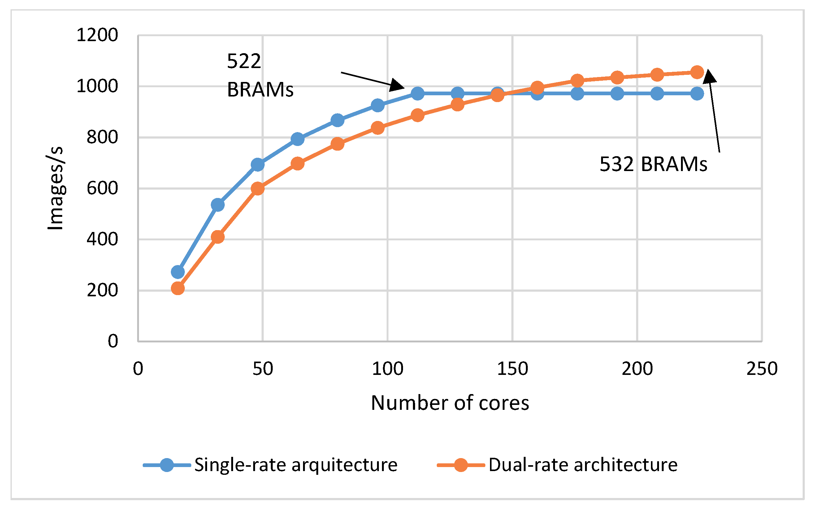
The best architectural option depends on the ratio between computational and on-chip memory resources. The performance breakthrough design point was estimated based on the performance and area models considering a maximum on-chip memory with the same size of the ZYNQ7045 (see Figure 11).

The performance breakthrough point is at around 150 cores, when the dual-rate architecture becomes faster than the single-rate solution. The increase in performance of the dual-rate architecture from this point on is not so evident because the execution becomes limited by the external memory bandwidth. Without this limitation, the scalability of the architecture would permit an almost linear increase in performance until reaching the parallelization limits.

The best architecture was compared with previous works implemented on a ZYNQ7045 for the same or smaller representations that consider other optimizations (see

Table 4. Performance comparison of the proposed architecture with previous works running AlexNet in ZYNQ7045 FPGA.

	[23] Baseline	[23]	[39]	This Work
Data format	$8\times 8$	[8, 2] bits	[4, 7] bits	$8\times 8$
LUTs	86,262	103,505	176,192	185,920
BRAMs	303	498	–	522
DSPs	808	550	900	704
BW	10.8	3.3	–	4.0
Freq	200	200	150	250
Images/s	340	856	854	967
GOPs	493	1240	1238	1401
GOPs/kLUTs	5.7	11.9	7.0	7.6
GOPs/DSPs	0.6	2.2	1.4	2
GOPs/BRAMs	1.6	2.5	–	2.7
TOP-1 accuracy	54.6%	52.6%	52%	54.7%

).

The works in [23,39] consider data size reduction of weights. Reducing the size of weights allows the reduction of required memory and the size of computation units. The first column considers a fixed data size of 8 bits, as the proposed architecture. In this case, our solution has a performance $2.8\times$ better with a smaller memory bandwidth. The baseline architecture from [23] was quantized with 8 bits in the first and last layers, 2 bits in convolutional layers and 1 bit in fully connected layers. Our solution is still faster than this proposal by about 13%; it is 2% more accurate but uses more resources. It is important to note that zero-skipping can be applied to hybrid quantized networks without any accuracy loss. In addition, the architectures proposed in [23,39] were only implemented in a medium density FPGA. Its pipelined structure limits its implementation in low density FPGAs. Our proposal can be implemented in any FPGA.

The area efficiency of our proposals is smaller than the compared works, since the proposed work deals with a larger data format and consequently the arithmetic units are larger. Besides, the other proposals implement pipelined structures with a module tailored for each layer, but require more memory to store weights for all layers and a complex access pattern to read the feature maps stored in external memory. This memory requirement limits its applicability to low density FPGAs.

8. Conclusions

This work describes an optimized architecture for the inference execution of CNN. The architecture targets low density FPGAs, that is, with low on-chip memory and low computational resources. To improve performance and reduce hardware, zero-skipping and weight pruning (static and dynamic) were applied with 8-bit fixed-point representation.

Compared to state-of-the-art works over the same FPGA devices, we were able to improve the throughput about $5.8\times$ in a ZYNQ7020 with less than 1% accuracy degradation. To show the scalability of the solutions, the architectures were designed for a ZYNQ7045. The improvements are smaller, compared to state of the art but still $1.13\times$. Besides the achieved performance, the results show that it is possible to run large networks in a low density FPGA with acceptable performance with small accuracy degradation.

Since the size of data has a great impact over the performance of the solution, future work will consider the integration of data size reduction techniques with the optimized architecture proposed in this work.