Magnetic Loss Analysis in Coaxial Magnetic Gears

Abstract

This paper proposes a procedure for computing magnetic losses in coaxial magnetic gears. These magnetic structures are made of permanent magnets and ferromagnetic poles in relative motion transferring torque between two shafts in a contactless way. The loss computation in magnetic materials is crucial to define the system performance. The flux distribution inside the iron parts is computed by means of the finite element method and a model of iron losses taking into account the rotational nature of the flux loci is applied. The procedure highlights where the major loss sources are present and gives the opportunity to evaluate some corrective measures to reduce their effects. Particular attention is devoted to the 2D modeling in presence of permanent magnets segmentation.

1. Introduction

Magnetic transmission is becoming an attractive technology for different industrial sectors where the matching between two rotating parts having different characteristics in terms of rated speed and torque is required. In particular, magnetic gears are encountering a growing interest in applications on electric and hybrid vehicles and wind turbines [1,2,3].

A magnetic gear comprises an inner and an outer rotor typically having surface mounted permanent magnets and a middle rotor made of ferromagnetic steel segments. The ferromagnetic steel segments modulate the magnetic field in order to allow the electromechanical interaction between the different rotors giving rise to the torque transmission. The principles of operation of the magnetic gears are better detailed in [4,5,6]. Thanks to the absence of contacts between the rotors, magnetic gears overcome several limitation presented by the classical mechanical gears such as mechanical friction and consequent wear, necessity of lubrication and maintenance, while they offer additional remarkable benefits: For instance, the inherent overload protection and self re-engaging when the overload torque is removed [7]. Thus, magnetic gears could be considered for substituting mechanical gearboxes when reliability and maintenance are key factors.

In order to assess the torque transfer in steady state conditions and to evaluate the dynamic behavior in transient settings, it is extremely important to model all the aspects of the energy conversion chain [8]. The one of magnetic loss evaluation is particularly difficult because the magnetic locus has a rotational shape in all of the iron regions. Previous papers assess power loss by measurement only [9,10]. In [11] only losses due to the eddy currents are taken into account. In [12], iron losses are considered and approximatively estimated through a Steinmetz approach.

In this paper a loss model tailored for rotational loci is adopted. This model is coupled with a simulation of the magnetic gear performed through finite element method. The results provide indications on the behavior of the power loss for each part of the machine.

The paper is organized as follows. The first part focuses on the machine modeling for the analysis through the finite element method. Both 2D and 3D formulations are introduced in Section 2. The results provided by the two models are compared in order to assess the validity of the 2D model for the loss computation. In Section 2.3 a method to take into account the effects of permanent magnets segmentation in the 2D model is presented and investigated. The used method for the loss computation is introduced in Section 3. The results of the power loss computation are presented and discussed in Section 4. Finally, the key results and contributions of the work are summarized in Section 5.

2. Magnetic Gear Model

The magnetic gears usually present a limited axial dimension as well as their standard mechanical counterpart. Moreover, the presence of the intermediate rotor constituted by the iron poles gives rise to a wide air gap and a consequent high reluctance path for the magnetic flux of the permanent magnets. 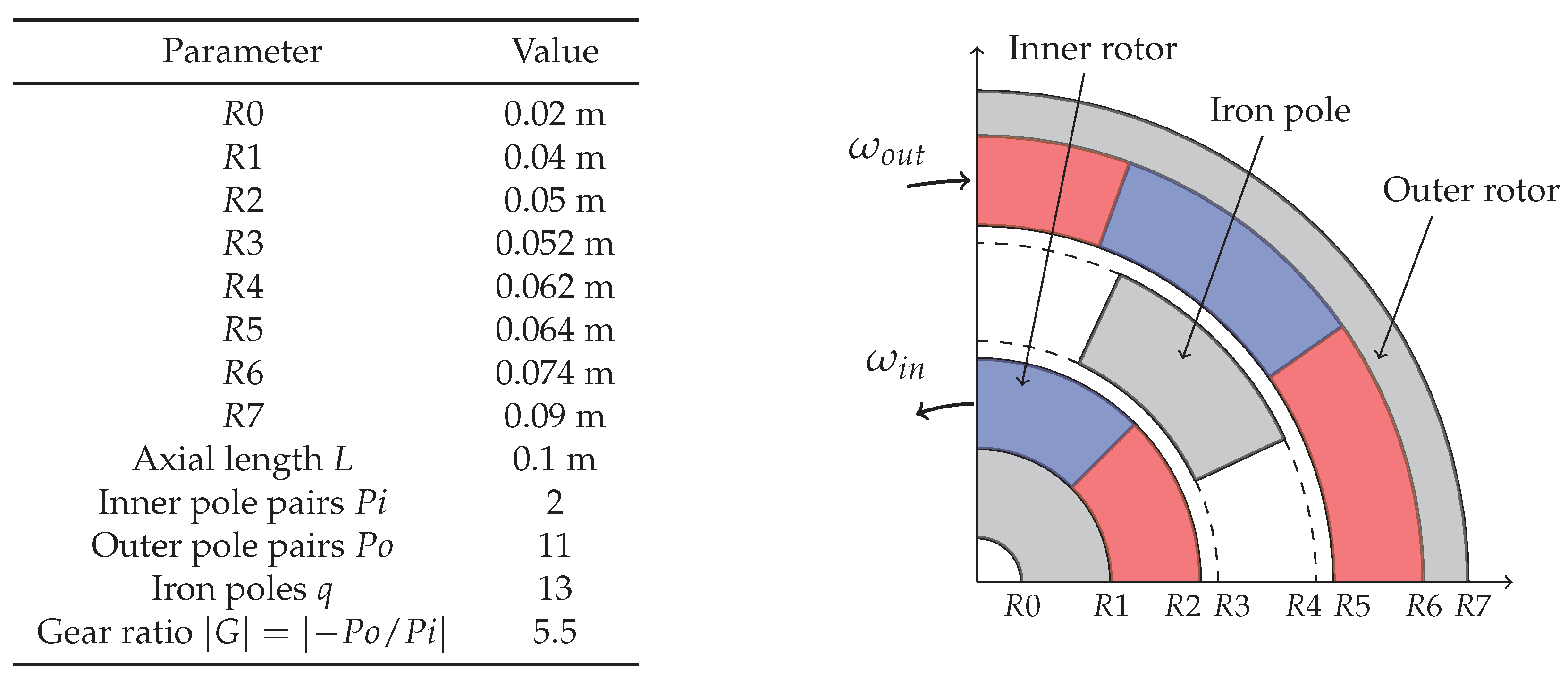According to these considerations, it is not easy to assert a priori if a 2D model of the machine can provide accurate enough results as typically happens for the classical electric rotating machines [13]. For this reason, a preliminary analysis has been carried out in order to compare the results in terms of magnetic flux distribution for a 3D and a 2D finite element model. The analysis is conducted considering the reference magnetic gear sketched in Figure 1. The magnets are considered to be made of NdFeB with conductivity $\sigma =0.65\mathrm{MS}/\mathrm{m}$ and residual magnetic flux density $B_{\mathrm{r}}=1.2\mathrm{T}$ while the iron poles and the yokes are considered made of non-oriented Fe-(3.2 wt %)Si sheet with thickness $d=0.356\mathrm{mm}$, electrical conductivity $\sigma =2.04\mathrm{MS}/\mathrm{m}$ and saturation polarization $J_s=2.01\mathrm{T}$.

2.1. 2D Model

The equations applied within the gear domain are the quasi-static Maxwell laws. In this paper, the magnetic field, flux density and current density will be referred as $\mathbf{H}$, $\mathbf{B}$ and $\mathbf{J}$.

Considering iron lamination, high permeability domains are modeled neglecting the eddy currents effects but considering the iron non-linearities $\mathbf{H}=\nu \left(\right|\mathbf{B}\left|\right)·\mathbf{B}$, where $\nu$ is the material reluctivity. The linear material law $\mathbf{B}=\mu ·\mathbf{H}+{\mathbf{B}}_{\mathbf{r}}$ is adopted for the permanent magnets (PMs), where $\mu$ is the magnet permeability and ${\mathbf{B}}_{\mathbf{r}}$ is the residual flux density. The current density term ${\mathbf{J}}_{\mathrm{e}}$ in the studied case is only constituted by eddy currents since there are no source terms due to windings. In the 2D case, the problem geometry allows the eddy currents to close at infinity if the current density integral over the cross section V of each magnet is not zero. In this case the overall value of the current density has to be constrained to be zero on each permanent magnet region by imposing the additional condition ${\int }_V{\mathbf{J}}_{\mathbf{e}}\mathrm{d}V=0$ for each permanent magnet. The $\mathbf{A}$ formulation in the ith PM is:

$$\left\{\begin{array}{c}\nabla \times (\nu \nabla \times \mathbf{A})=-\sigma {\displaystyle \frac{\partial \mathbf{A}}{\partial t}}-\sigma {\displaystyle \frac{V_{\mathrm{PM}}^i}{L}}{\mathbf{e}}_{\mathbf{z}}+\nabla \times \left(\nu {\mathbf{B}}_{\mathbf{r}}\right)\\ {\displaystyle {\int }_V{\mathbf{J}}_{\mathbf{e}}\mathrm{d}V}={\displaystyle {\int }_V\left(-\sigma {\displaystyle \frac{\partial \mathbf{A}}{\partial t}}-\sigma {\displaystyle \frac{V_{\mathrm{PM}}^i}{L}}{\mathbf{e}}_{\mathbf{z}}\right)\mathrm{d}V}=0\end{array}\right.$$

(1)

where $\mathbf{A}=\left(0,0,A_z\right)$, $\sigma$ is the magnet conductivity, L is the machine length, $-\sigma \frac{V_{\mathrm{PM}}^i}{L}{\mathbf{e}}_{\mathbf{z}}$ is the additional current density term and $V_{\mathrm{PM}}^i$ is the equivalent voltage drop across the $i^{th}$ PM that ensures the net zero current property. The formulation of Equation (1) has been implemented in Comsol Multiphysics software.

2.2. 3D Model and Comparison

The formulation adopted for the 3D modeling is standard, based on the magnetic vector potential $\mathbf{A}$ and the scalar electric potential V on the conductive permanent magnet regions, while the scalar magnetic potential is adopted in the current-free regions [14].

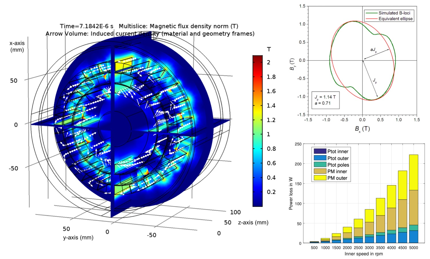
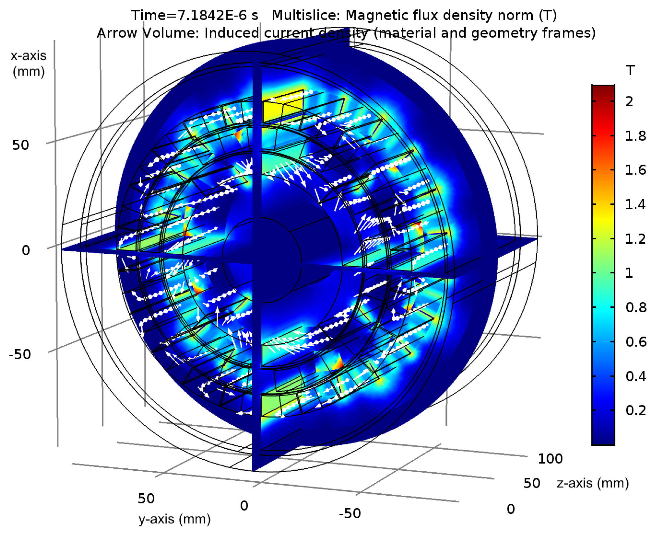
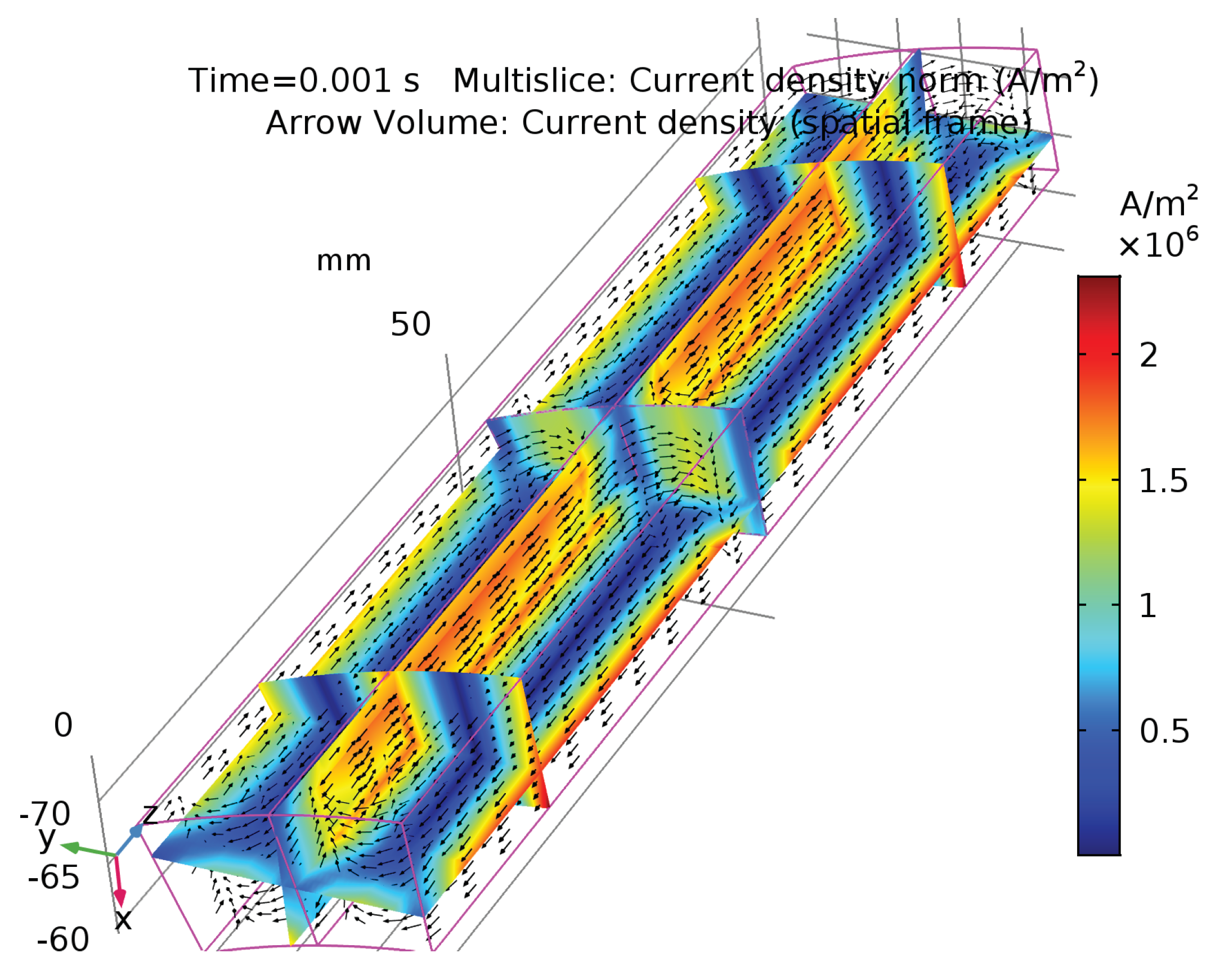
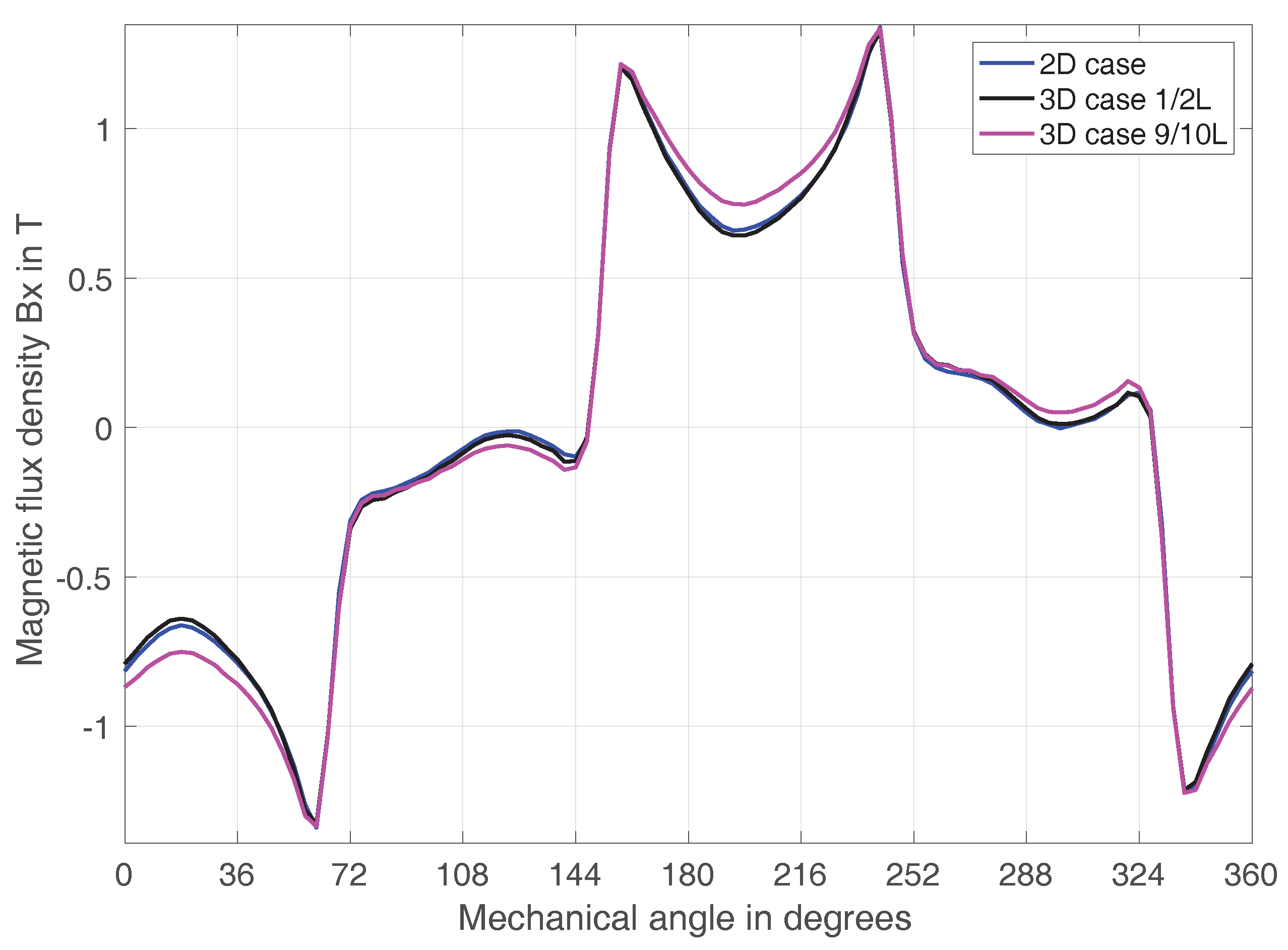
An example of magnetic flux density norm and the induced eddy currents of the 3D model is shown in Figure 2: Since the machine is not periodic, the whole geometry needs to be modeled, leading to a problem that is computationally intensive. These results computed in different sections of the machine are compared with the ones provided by the 2D model for its three main gear parts.

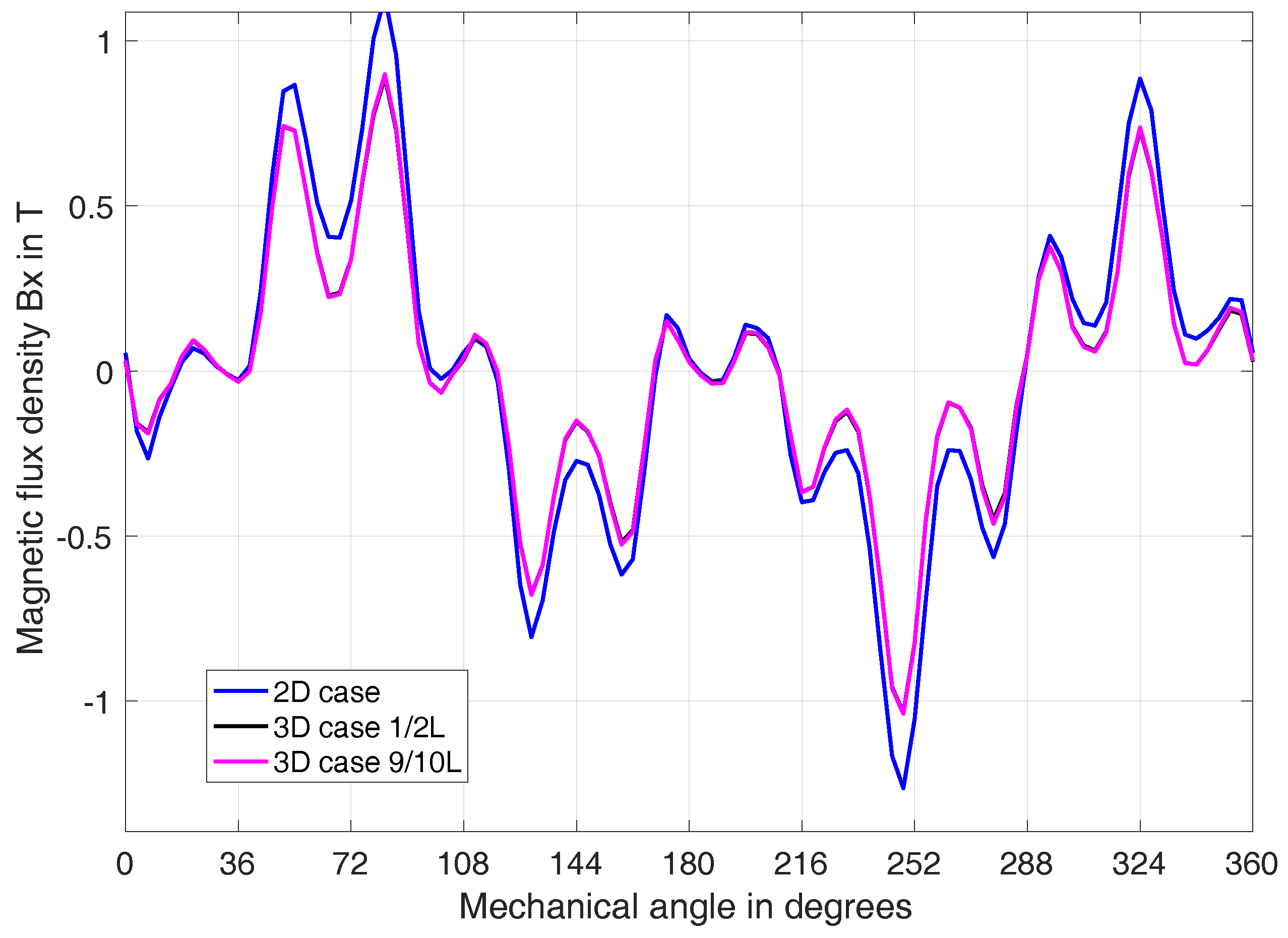
Figure 3, Figure 4 and Figure 5 show the comparisons of the flux density values along arcs taken inside the inner rotor, outer rotor and (non-linear) iron poles, respectively. In each plot three curves are displayed, one for the 2D case and the others for the 3D case where the query points lie on two slices located at $z=L/2$ (in the middle of the axial length of the machine) and $z=9L/10$ (close to the machine edge). Some unphysical peaks are visible in Figure 5. These peaks are due to the rather coarse 3D model mesh which had to be used in order to limit the computational requirements: the 3D model has 542,000 degrees of freedom (DOFs), while the 2D model has 40,000 DOFs. For both cases the time step is adaptive based on the backward differentiation method.

The comparison shows anyway a good match between 2D and 3D simulations, especially as far as the main quantities are concerned. In

Table 1. Flux density norm comparison between 3D and 2D simulations.

Slice	Norm Ratio |ΔB|
$z=L/2$	$13.6\%$
$z=9L/10$	$18.3\%$

the norm of the difference vector

$$|\Delta \mathbf{B}|={\displaystyle \frac{\Vert {\mathbf{B}}_{3\mathrm{D}}-{\mathbf{B}}_{2\mathrm{D}}\Vert }{\Vert {\mathbf{B}}_{3\mathrm{D}}\Vert }}$$

(2)

is reported, where $\mathbf{B}$ is a vector containing the flux density norm in all query points. The difference vector is higher if the slice is close to the machine edge rather than the machine center, since some flux lines close in the air. However, the 2D approximation is still satisfactory. These considerations suggest that the loss estimation can be effectively computed, thus the loss estimation is based on the flux density computed from 2D simulations.

2.3. Permanent Magnets Segmentation

As typically done in the domain of the electric rotating machines, also for the magnetic gears the magnetic transmission efficiency can be considerably increased by means of the segmentation of the PMs. The segmentation aims to lower the overall PMs conductivity reducing the related eddy current losses and it is commonly done both along the circumferential and the axial direction. Clearly, the segmentation introduces three-dimensional effects that cannot be directly evaluated by using a 2D model. Among the previous works that addressed this issue, ref. [15] proposes to study the effects of the circumferential segmentation through the adoption of analytical models by which the loss decay rate can be computed as a function of the PMs segments number, avoiding the 3D segmentation modeling. By following this approach, it is proven that the power loss decays quadratically with the number of circumferential segments.

A similar approach is here proposed in order to take into account both the effects of circumferential and axial segmentation. The method consists in the adoption of equivalent conductivities ${\sigma }_{\mathrm{PMin}}$ and ${\sigma }_{\mathrm{PMout}}$, for the inner and outer rotor respectively, that are fractions of the original conductivity of the PMs material. The value of the equivalent conductivities is derived from the comparison with the 3D model. The results of this comparison are reported in

Table 2. Comparison of the permanent magnets (PMs) losses at ${\omega }_{\mathrm{in}}=5000\mathrm{rpm}$ with no segmentation and with circumferential (C) or axial (A) segmentation.

Model	Inner Rotor PMs Segmentation	Outer Rotor PMs Segmentation	${\mathit{\sigma }}_{\mathbf{PMin}}$	${\mathit{\sigma }}_{\mathbf{PMout}}$	${\mathit{P}}_{\mathbf{PMin}}$ (W)	${\mathit{P}}_{\mathbf{PMout}}$ (W)
3D	No	No	$\sigma$	$\sigma$	230	560
3D	2C.	2C.	$\sigma$	$\sigma$	220	160
3D	2A	2A	$\sigma$	$\sigma$	209	490
3D	2A + 2C	2A + 2C	$\sigma$	$\sigma$	205	155
3D	2A + 3C	2A + 3C	$\sigma$	$\sigma$	190	77
3D	2A + 14C	2A + 3C	$\sigma$	$\sigma$	87.5	77
2D	No	No	$\sigma /1.2$	$\sigma /1.52$	252	620
2D	2C	2C	$\sigma /1.6$	$\sigma /5.5$	221	165
2D	2A	2A	$\sigma /1.8$	$\sigma /1.9$	205	488
2D	2A + 2C	2A + 2C	$\sigma /1.95$	$\sigma /6$	206	155
2D	2A + 3C	2A + 3C	$\sigma /2.28$	$\sigma /11.7$	187	78
2D	2A + 14C	2A + 3C	$\sigma /4.5$	$\sigma /11.7$	87	78

. In this evaluation, the PMs Joule losses are computed considering different directions of segmentation and number of segments for an inner rotor speed ${\omega }_{\mathrm{in}}=5000\mathrm{rpm}$. In the 3D model, all the PMs segments are considered as insulated parts.

The physical effects of the segmentation with two axial segments and two circumferential segments are shown in Figure 6 and Figure 7 for outer permanent magnets and inner permanent magnets respectively. These figures show that the segmentation is much more effective for the outer PMs while the losses are lowered by a smaller factor for the inner PMs. In the case of the outer rotor, shown in Figure 6, the eddy current is evenly distributed in the segments. Conversely, Figure 7 shows that in the inner permanent magnets the eddy currents distribution locally concentrates in correspondence of the stationary pole pieces. In this case, the loss reduction is less effective as the adopted segmentation of the inner magnets gives rise to segments wider than the concentration regions.

By collecting the results reported in Table 2, it is possible to obtain the behavior of the PMs losses as a function of the number of circumferential segmentations shown in Figure 7. For convenience, the analyzed points are interpolated through a fitting function in order to better point out the losses trend. Figure 8 indicates that, despite the circumferential segmentation allows to strongly decrease the PMs losses, it starts to be less effective after a certain number of segments.

On the base of the discussed results, the overall loss evaluation is carried out in the following by considering a magnetic gear having 2 axial segmentations and 14 circular segmentations for the inner magnets, 2 axial segmentations and 3 circular segmentations for the outer magnets. This kind of segmentation gives rise to comparable segments surface for inner and outer PMs. In the 2D model, this means to consider an equivalent conductivity of the inner rotor PMs ${\sigma }_{\mathrm{PMin}}=\sigma /4.5$ and an equivalent conductivity of the outer rotor PMs ${\sigma }_{\mathrm{PMout}}=\sigma /11.7$. Hence, the latter are the values of PMs conductivity adopted for the loss computation.

3. 2-Dimensional Loss Model

The formulation of a comprehensive two-dimensional magnetic hysteresis model of magnetic sheets by which the loss might be calculated under arbitrary polarization loci (alternating, circular, elliptical, etc.) and time behavior has been accomplished to little extent so far. However, a rational approach to the 2D magnetic losses and their frequency dependence can be pursued in non-oriented (NO) steel sheets following the method and the tools proposed in [16,17,18] based on the statistical theory of loss of Bertotti [19]. This method is based on the concept of loss separation, by which the total loss W is expressed as the sum of the hysteresis $W_{\mathrm{hyst}}$, excess $W_{\mathrm{exc}}$, and classical $W_{\mathrm{class}}$ components, i.e.,

$$W=W_{\mathrm{hyst}}+W_{\mathrm{exc}}+W_{\mathrm{class}},$$

(3)

and the connection with their unidirectional (scalar) counterpart by an equivalent ellipsoid.

Following this approach, the hysteresis loss for a given elliptical flux locus is expressed as:

$$W_{\mathrm{hyst}}\left(J_p,a\right)\simeq W_{\mathrm{hyst}}^{\left(ALT\right)}\left(J_p\right)+W_{\mathrm{hyst}}^{\left(ALT\right)}\left(a{J}_p\right)\left(R_{\mathrm{hyst}}\left(J_p\right)-1\right)$$

(4)

where $R_{\mathrm{hyst}}=W_{\mathrm{hyst}}^{\left(ROT\right)}/W_{\mathrm{hyst}}^{\left(ALT\right)}$ is the experimental ratio between the hysteresis losses obtained under circular and alternating polarization, $J_p$, expressed as $J_p=B_p-{\mu }_0{H}_p$, is the peak polarization measured along the major axis of the ellipse, and a is the ratio between minor to major axis lengths. If $a=0$ only alternating loss is present while $a=1$ means purely rotating loss. Figure 9 shows the experimental behavior of $W_{\mathrm{hyst}}^{\left(ROT\right)}$, $W_{\mathrm{hyst}}^{\left(ALT\right)}$ and the ensuing ratio $R_{\mathrm{hyst}}\left(J_p\right)$ versus $J_p/J_s$ for the adopted steel (NO Fe-(3.2 wt%)Si sheet, thickness $d=0.356\mathrm{mm}$, $\sigma =2.04\mathrm{MS}/\mathrm{m}$, $J_s=2.01\mathrm{T}$). The experimental data are retrieved from [20]. It is worth noting that, as demonstrated in [21], the ratio $R_{\mathrm{hyst}}\left(J_p\right)$ can be assumed as generally valid for any ferromagnetic material at different sheet thicknesses and lamination types.

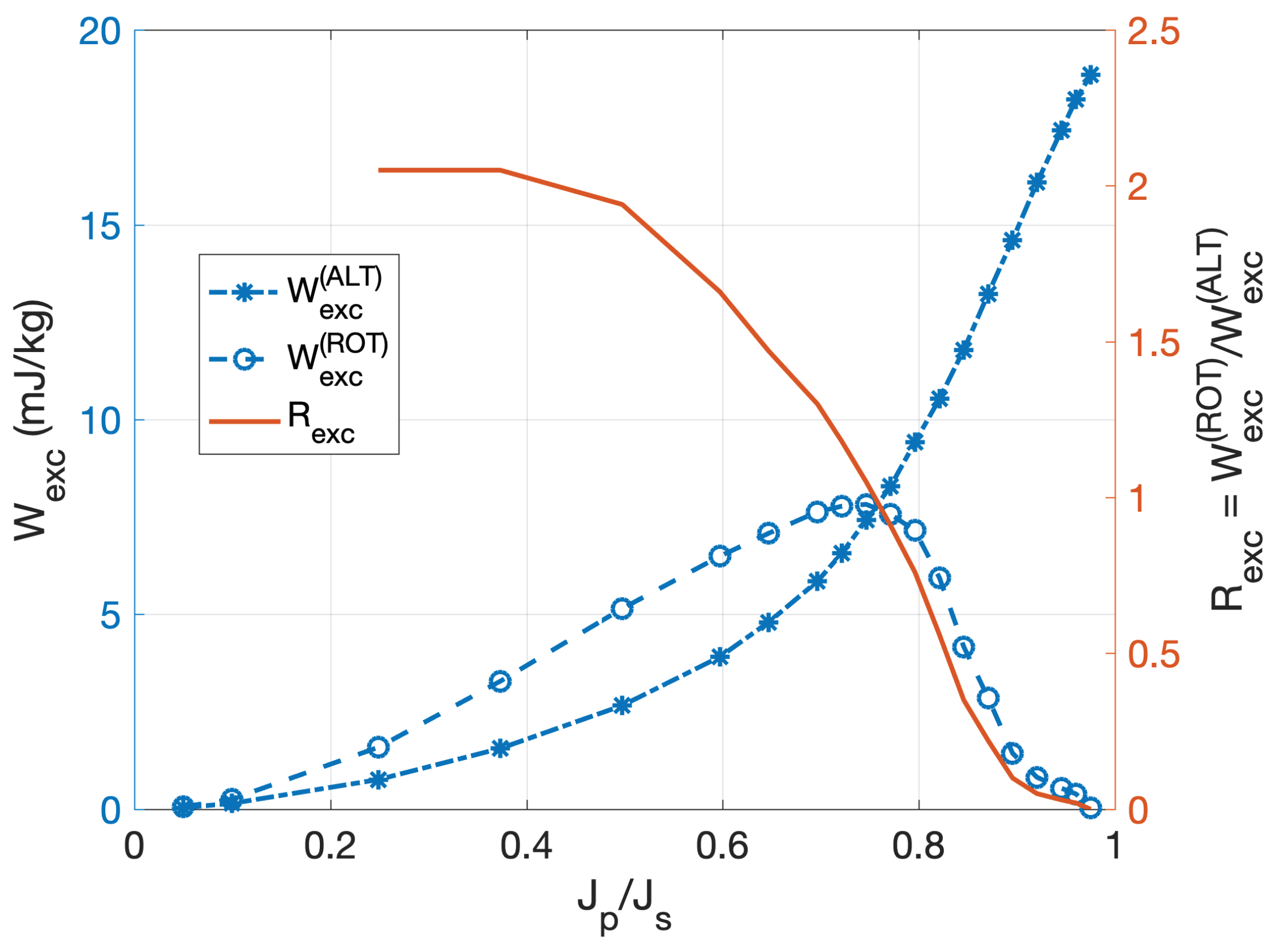
The excess loss is expressed as:

$$\begin{array}{c}{W}_{\mathrm{exc}}(J_p,a,f)\simeq g\left(a\right){\displaystyle \frac{\sqrt{f}}{\sqrt{f_0}}}·\left\{W_{\mathrm{exc}}^{\left(ALT\right)}(J_p,f_0)+W_{\mathrm{exc}}^{\left(ALT\right)}(a{J}_p,f_0)\left[{\displaystyle \frac{R_{\mathrm{exc}}\left(J_p\right)}{g\left(1\right)}}-1\right]\right\}\hfill \end{array}$$

(5)

where $W_{\mathrm{exc}}^{\left(ALT\right)}(J_p,f_0)$ is the excess loss obtained under alternating conditions at peak polarization $J_p$ and at the reference frequency $f_0=50\mathrm{Hz}$, $R_{\mathrm{exc}}\left(J_p\right)$ is the experimental ratio, at a given frequency, between the excess loss obtained under circular and alternating polarization and the function:

$$g\left(a\right)=\frac{\sqrt{2\pi }}{8.76}{\int }_0^{2\pi }{\left({\sin }^2\left(\phi \right)+a^2{cos}^2\left(\phi \right)\right)}^{3/4}\mathrm{d}\phi$$

(6)

The function $g\left(a\right)$ calculated for circular polarization $(a=1)$ is $g\left(1\right)=1.8$. Figure 10 shows, for the same material, the experimental behavior of $W_{\mathrm{exc}}^{\left(ROT\right)}$, $W_{\mathrm{exc}}^{\left(ALT\right)}$ and their ratio $R_{\mathrm{exc}}\left(J_p\right)$ versus $J_p/J_s$ [20]. It is worth noting that the ratio $R_{\mathrm{exc}}\left(J_p\right)$ is to a good extent independent of the frequency. The effect of time harmonic distortion on excess loss is here neglected as, in this specific case, it results in a marginal part of the total loss [22].

The classical loss, under negligible skin effect, at frequency f is obtained as:

$$W_{\mathrm{class}}={\displaystyle \frac{\sigma d^2}{12}}{\int }_0^{1/f}\left[{\left(\frac{\mathrm{d}{B}_x}{\mathrm{d}t}\right)}^2+{\left({\displaystyle \frac{\mathrm{d}{B}_y}{\mathrm{d}t}}\right)}^2\right]\mathrm{d}t$$

(7)

where $B_x\left(t\right)$ and $B_y\left(t\right)$ are the induction components along x and y axis respectively.

The previous formulas are used to evaluate the losses in the iron poles. As the loci of magnetic flux density are not always elliptical due to harmonic distortion and geometrical effects, a simulated ellipse equivalent to the actual one is generated for every point in the pole keeping as fixed the peak of the polarization and the area of the locus. On this equivalent locus, the parameter a is computed. An example of this simulated ellipse is reported in Figure 11.

4. Losses vs. Speed

Similarly to the electric rotating machines, the power loss depends on the rotational speed and also on the load angle ${\theta }_{\mathrm{L}}$ (i.e., the phase shift between the first harmonic of the rotating magnetic fields generated by the inner and the outer rotor, respectively):

$${\theta }_{\mathrm{L}}={\theta }_{\mathrm{in}}-{\theta }_{\mathrm{out}}·\left(-{\displaystyle \frac{Po}{Pi}}\right)={\theta }_{\mathrm{in}}-{\theta }_{\mathrm{out}}·G.$$

(8)

In this section, the results relative to the maximum torque capability are shown. A great part of the iron loss has to be attributed to iron poles as they are subject to high flux densities that, as shown in the previous section, show rotational behavior. The iron yokes are interested by the superposition of fields with periodicity $Pi$ and $Po$, hence rotational loci are also expected even if the area enclosed by the loop is smaller than the one of the iron poles and a DC bias is present. The loci frequency in the gear components, at ${\omega }_{\mathrm{in}}=5000\mathrm{rpm}$, ${\omega }_{\mathrm{poles}}=0\mathrm{rpm}$, ${\omega }_{\mathrm{out}}=-909.09\mathrm{rpm}$, reads:

$$\left\{\begin{array}{c}{f}_{\mathrm{poles}}={\displaystyle \frac{{\omega }_{\mathrm{in}}}{60}}Pi\hfill \\ f_{\mathrm{in}\mathrm{yoke}}={\displaystyle \frac{{\omega }_{\mathrm{in}}}{60}}q\hfill \\ f_{\mathrm{out}\mathrm{yoke}}={\displaystyle \frac{{\omega }_{\mathrm{in}}}{60}}{\displaystyle \frac{Pi·q}{Po}}\hfill \end{array}\right.\stackrel{}{\to }\left\{\begin{array}{c}{f}_{\mathrm{poles}}=167\mathrm{Hz}\hfill \\ f_{\mathrm{in}\mathrm{yoke}}=1083\mathrm{Hz}\hfill \\ f_{\mathrm{out}\mathrm{yoke}}=197\mathrm{Hz}\hfill \end{array}\right..$$

(9)

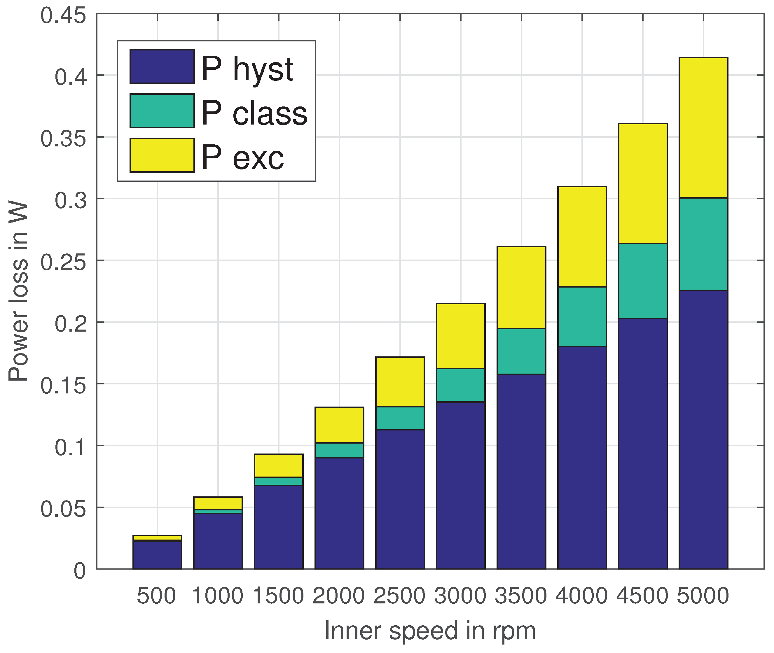
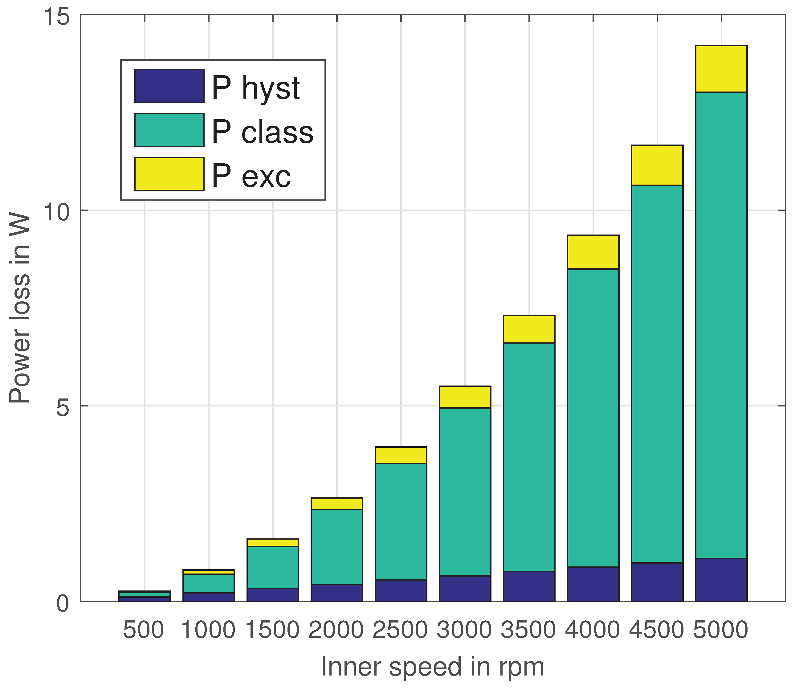
Figure 12 shows the losses components in the inner yoke versus the inner rotational speed. The classical Steinmetz frequency dependency applies to the plot: The hysteresis loss grows linearly with the rotational speed, the classical component quadratically and the excess component as ${\omega }_{\mathrm{in}}^{1.5}$. The hysteresis loss is the predominant term with lamination thickness $\delta =0.356\mathrm{mm}$.

Figure 13 shows the losses components in the outer yoke and the same considerations of Figure 12 applies. The absolute loss value differs by two orders of magnitude in comparison to the previous case. This happens because of the bigger iron volume and because the inner rotor magnetic field has a strong influence on the outer loci while, on the contrary, a great part of the flux lines of the outer rotor magnets close on the iron poles without affecting the inner yoke.

Figure 14 shows the losses in the iron poles: the eddy current loss is the predominant one, while the hysteresis and excess relative contributes are lower than in the inner and outer yoke cases. This is due to the change in the loss mechanism: because of the reduced volume, the flux density in the iron poles is higher than the yokes. At these $J_P$ values, according to Figure 9 and Figure 10, the loss contributions drop due to the rotational component of flux density and this explains the smaller contributions of excess and hysteresis loss.

As a final evaluation, Figure 15 shows the total losses on inner and outer yokes, iron poles and permanent magnets. The inner yoke losses are negligible while the PMs losses are not, since their value is higher than the one of the iron losses in ferromagnetic part.

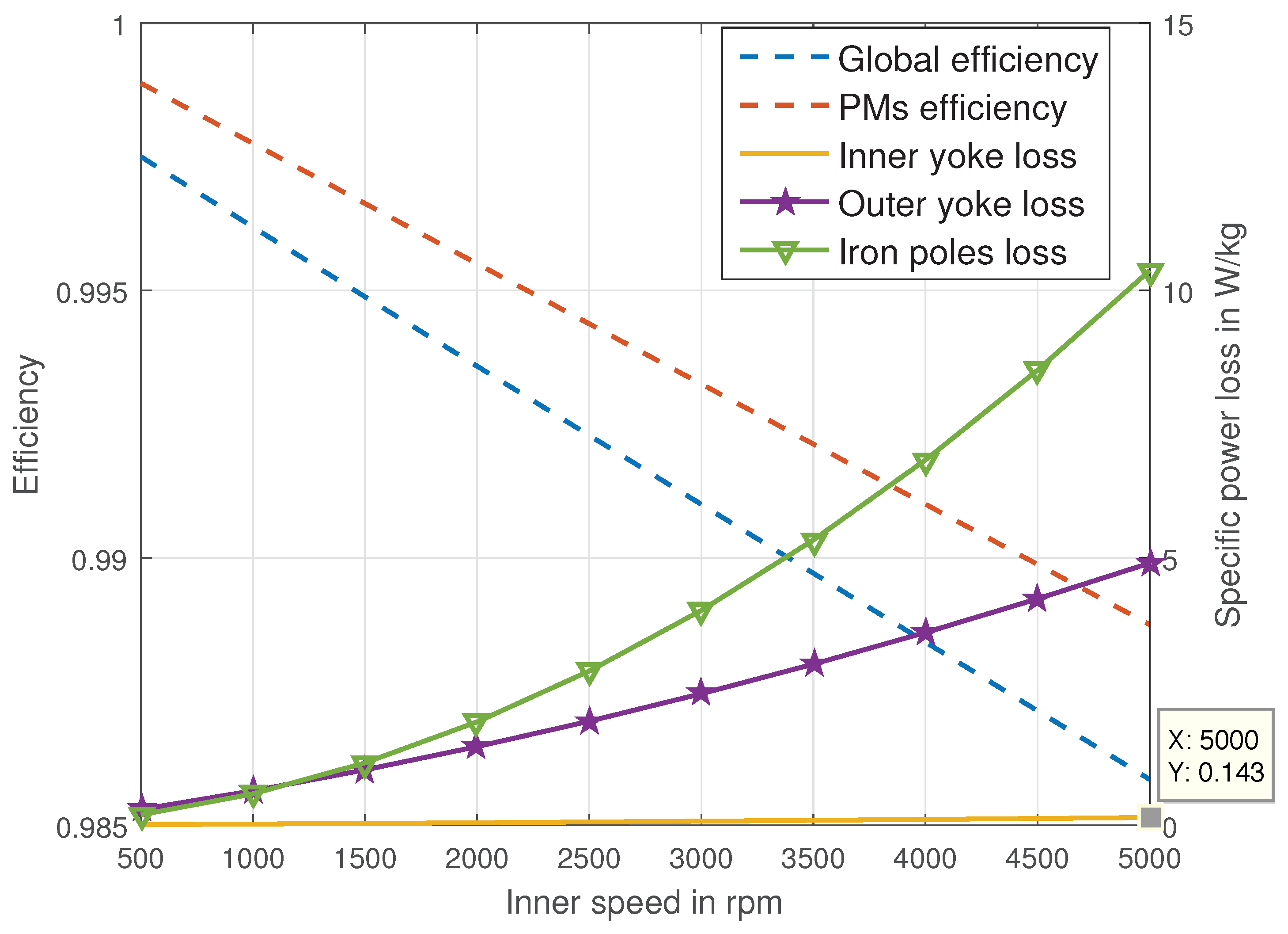
Finally, Figure 16 shows the global efficiency plot, the PMs efficiency (i.e., the ratio between power loss in PMs and transferred mechanical power) contribution and the specific power losses in the iron domains. The highest specific loss is obtained in the iron poles. This high specific loss has to be expected in any case as the iron poles are the elements subject to the highest magnetic induction at the highest harmonic content.

5. Conclusions

This paper has presented a model for the losses estimation in magnetic transmission. The magnetic gear is modeled through the finite element method and the equations for the loss calculation with rotational flux loci are discussed. The comparison between 3D and 2D simulations confirmed that the 2D modeling can provide effective results indicating that the edge effects of the machine can be neglected. A simplified method allowed to take into account the effect of PMs segmentation also in the 2D model by using two equivalent conductivities for inner and outer rotor permanent magnets.

The efficiency and losses plots have been shown for different speeds at the maximum load capability. The results indicate that the maximum specific iron losses are located in the iron poles as they are interested by induced current density showing the higher rotational component. These preliminary evaluations, as well as the final results, indicated that the PMs segmentation represents an effective way to further increase the transmission efficiency. It is proven that, for an equal number of segments for outer and inner PMs, this technique is more effective in the outer rotor according to the wider area covered by the inner rotor magnets. Moreover, the results have shown that the circumferential-segmentation is more effective than the axial one.