Article

On Inferring Intentions in Shared Tasks for Industrial Collaborative Robots

Institut de Robòtica i Informàtica Industrial, CSIC-UPC, Llorens i Artigas 4-6, 08028 Barcelona, Spain
*
Author to whom correspondence should be addressed.
Electronics 2019, 8(11), 1306; https://doi.org/10.3390/electronics8111306
Submission received: 29 September 2019 / Revised: 30 October 2019 / Accepted: 1 November 2019 / Published: 7 November 2019
(This article belongs to the Special Issue Cognitive Robotics & Control)

Abstract

:
Inferring human operators’ actions in shared collaborative tasks plays a crucial role in enhancing the cognitive capabilities of industrial robots. In all these incipient collaborative robotic applications, humans and robots not only should share space, but also forces and the execution of a task. In this article, we present a robotic system that is able to identify different human’s intentions and to adapt its behavior consequently, only employing force data. In order to accomplish this aim, three major contributions are presented: (a) a force based operator’s intention recognition system based on data from only two users; (b) a force based dataset of physical human–robot interaction; and (c) validation of the whole system with 15 people in a scenario inspired by a realistic industrial application. This work is an important step towards a more natural and user-friendly manner of physical human–robot interaction in scenarios where humans and robots collaborate in the accomplishment of a task.

1. Introduction

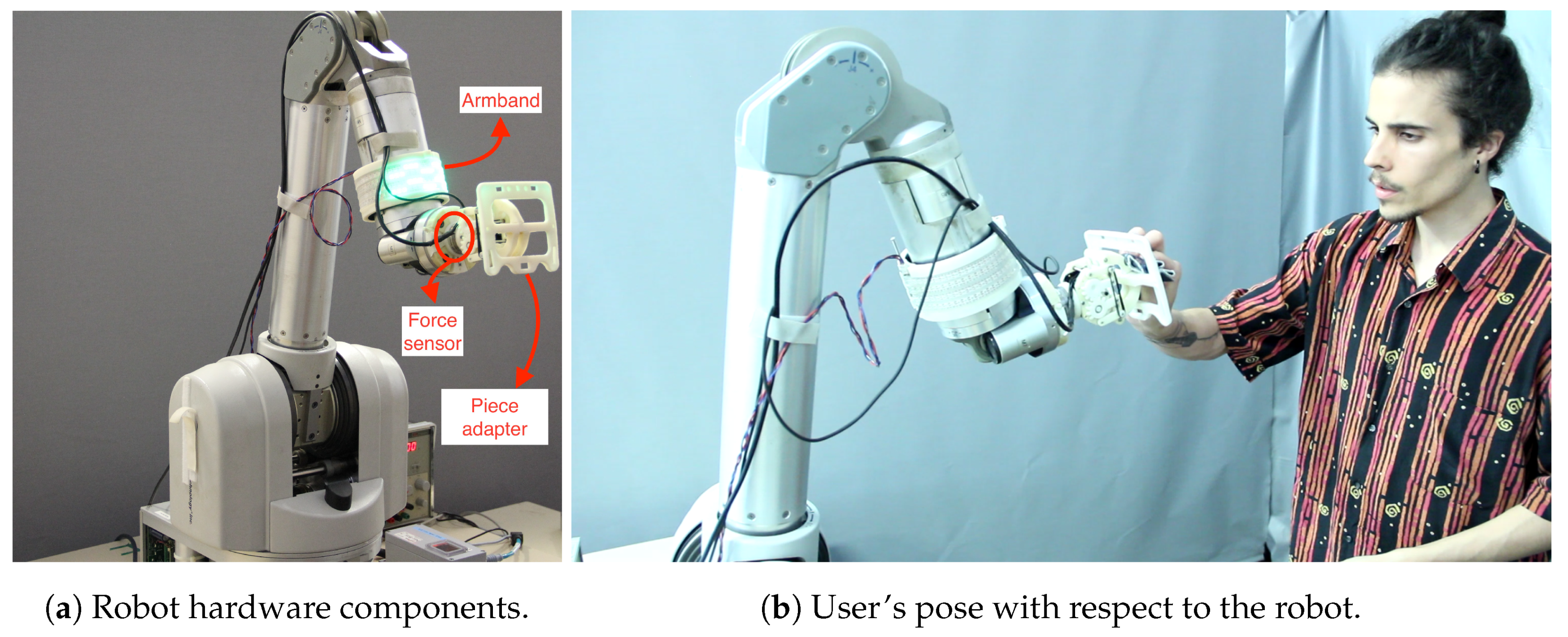
Currently, there is a rising trend towards smart factories where all the involved entities cooperate and communicate with each other. This is often referred to as Industry 4.0 or the fourth industrial revolution. Settling this aim for the industrial robotics sector would require freeing robots from their current work cells, closer to operators, compromising human safety [1,2]. In the interest of overcoming those safety issues, over the last few years, collaborative robots or cobots have emerged [3,4,5]. These robots are specifically designed for direct interaction with a human within a defined collaborative workspace [6]. Collaborative robots have meant great progress towards a safer coexistence of operators and industrial robots. Nevertheless, scenarios where humans and robots exchange forces and share the execution of a task require the use of robots equipped with complex cognitive capabilities [7]. Bauer et al. [8] proposed five levels of cooperation between robots and humans (see Figure 1). The authors stated that most of the current real applications of industrial robots are based on the cooperation levels coexistence and synchronized [9,10]. Driven by the lack of applications where more complex levels of cooperation are addressed, we propose a scenario based on the fifth level, collaboration. Figure 2 depicts the proposed setup, where a human and a robot exchange forces while sharing the execution of a task inspired by a realistic industrial scenario.
In a real industrial environment, operators tend to suffer from injuries related to the usual repetitive tasks involved in their daily duties. In our scenario, it is important to reduce as much as possible very mechanical movements and let the users interact with the robot through more natural kinds of gestures. Moreover, the cooperation between the human and the robot during repetitive physical human–robot interactions should be fluent [1,6]. Based on our experience, one second is the maximum amount of time for an efficiently responsive human–robot collaboration. In industrial surroundings, there is much heterogeneous contextual information that can have an effect on or modify the progress of a task. In future work, we would like to benefit from using that contextual information. Therefore, it would be desirable that our machine learning approach be able to cope with not only temporal sequences, but also other types of environmental variables. To sum up, natural interaction, fast prediction, and contextual variables will play a relevant role for the data gathering and the selection of the most appropriate approach.
The main contributions presented within this work are:
  • Force based operator’s intention inference. We implemented two different approaches, and both were thoroughly evaluated and compared. Finally, one of them was selected and used during the validation with users. Inference time and the possibility of including contextual information were considered for the comparison. The first approach consisted of a k-nearest neighbor classifier, which uses as the metric dynamic time warping. In this case, the time series data are directly fed to the classifier. The second approach was based on dimensionality reduction together with a support vector machine classifier. The reduction was performed over the concatenation of all force axes of the raw time series.
  • Force based dataset of physical human–robot interaction. Due to the lack of similar existent datasets, we present a novel dataset containing force based information extracted from natural human–robot interactions. Geared towards the inference of operators’ intentions, the dataset comprises labeled signals from a force sensor. We aimed to generalize from a few users to several. Therefore, our dataset was only recorded with two users. Indeed, this is compliant with industrial environments in which the system should be used by new operators, preferably with no need for retraining.
  • Validation in a use-case inspired by a realistic industrial collaborative robotic scenario. The performance of the selected approach was evaluated in an experiment with fifteen users, who received a short explanation of the collaborative task to execute. The goal of the shared task was to inspect and polish a manufacturing piece where the robot adapted to the operator’s actions. To generalize, recall that the model was trained with data from only two users, while it was evaluated against other fifteen users.
The remaining content of the paper is structured as follows. Section 2 provides an analysis of the current state-of-the-art related to the topic covered in this document. The data acquisition process and dataset specifications are introduced in Section 3. In Section 4, we explain the implementation, evaluation, and comparison of the two approaches to the force based operator’s intent inference. The validation of the proposed system is presented in Section 5, and the conclusions and future work are discussed in Section 6.

2. Related Work

In this work, we are primarily interested in exploring force based industrial collaborative robotic tasks, that is those in which the physical interaction plays an essential role in the accomplishment of the task. In particular, it is of great interest for us to carry out a twofold research of: (a) applications where humans physically interact with robots; and (b) datasets containing force based information extracted from human–robot interaction scenarios.
In the literature, several works have presented applications where humans and robots physically interact. However, it is difficult to find recent works where, as in ours, the physical interaction plays a major role in the execution of a shared task. Indeed, in most of the cases, the force exchange between humans and robots is ignored or undesired. Hence, we analyzed two groups of works: (a) those in which the physical interaction is ignored or undesired; and (b) those in which the robot uses the force based information to adapt its state. Regarding the first group of works, Cherubini et al. [11] discussed a collaborative scenario where a human and a robot shared the task of Rzeppa homokinetic joint insertion. In this case, even though there was an exchange of force, unlike in our work, the robot just remained stiff and did not use the force based information to adapt its state. Maurtua et al. [12] described a set of experiments aimed at measuring the trust of workers on fenceless human–robot industrial collaborative applications. In all the experiments, the force was undesired; thus, the robot stopped when an external force was detected. De Gea Fernández et al. [13] described another industrial situation in which two robotic arms collaborated with an operator. The robots avoided the physical interaction with the human as long as possible, and when a physical interaction occurred, they remained in a compliant mode so that the force was ignored. Raiola et al. [14] addressed the problem of learning virtual guiding fixtures, analogous to the use of a rule when drawing, in human–robot collaboration. Even though there was physical interaction during the task execution, the robot did not use the force based information while guiding the human. In the work presented by Munzer et al. [15], a human and a robot performed sub-tasks of a shared task: wooden box assembling. The robot and the human shared forces, and the robot was able to adapt to the situation, but not using the force, just using vision, or being explicitly asked to do it by voice commands or instructions using a graphical interface. Some recent works presented cases in which robots adapted their behavior based on the physical interaction between humans and robots. Peternel et al. [16] proposed to estimate human fatigue to adapt how much a robot is helping in human–robot collaborative manipulation tasks: sawing and surface polishing. Rozo et al. [17] proposed a framework for a user to teach a robot collaborative skills from demonstrations. Specifically, they presented an approach that combined probabilistic learning, dynamical systems, and stiffness estimation, to encode the robot behavior along with the task. Hence, the method allowed a robot to learn not only trajectory following skills, but also impedance behaviors. Unlike in our work, in these two works, the adaptation was done at the low-level control of the robot by a hybrid force/impedance controller, while we did it at the symbolic level of the task. A scenario where a human and a robot physically interact through a handover of an object was discussed by Mazhar et al. [18]. Force signals were used to identify different phases of the sequence of actions. When a force threshold was exceeded, the system interpreted that the robotic hand should close to grasp the object during the handover. Zhao et al. [19] presented an operator’s intention recognition approach inspired by a collaborative sealant task. The intentions, rather similar to ours, were also used to adapt the state of the robot, just as in our work. However, the interactions they proposed were simplistic as the classes could be discriminated between them with thresholds in the force. In our work, we recorded two different datasets, one that was similar to theirs, containing simpler mechanical movements, and another one that included more natural human–robot interactions. The latter was used during the experiments. Gaz et al. [20] presented a new robot control algorithm aimed at being used in a scenario where a robot grasps a piece while the operator polishes it. The proposed collaborative task was the same we used, but they considered only two robot modes: (a) stiffness, while the user polishes’ and (b) compliance, while the user modifies the orientation of the end effector. Unlike in our work, there was no classification of the user’s intentions; the force was directly applied to different parts of the robot: (a) a force sensor fastened to the robot’s wrist; and (b) the rest of the robot’s joints. Losey et al. [21] presented a comprehensive review of intent detection and other aspects within the context of shared control for physical human–robot interaction. Especially interesting was how this paper was structured, talking about three aspects covered in our work: (a) user intent recognition; (b) shared control between humans and robots; and (c) methods to inform the human operator about the robot’s state.
In the literature, there are datasets extracted from robotics scenarios in which either the human–robot interaction is not physical or the force based tasks do not include interaction with humans. The former correspond to social robotics scenarios, where the most common means of interaction is not physical, but verbal. Those datasets usually contain video, speech (audio and transcripts), robot joint-sate, physiological data (e.g., bio-signals), or subjective data in the form of questionnaires [22,23,24,25,26]. On the other hand, it is possible to find some datasets containing force/torque data extracted from robotic scenarios in which robots and humans do not interact. Yu et al. [27] presented a dataset in the context of pushing tasks where a robot pushed an object along a specific surface. For each combination of an object’s shape and a surface’s material, these data contained forces in the pusher and poses of both the object and the pusher. Another interesting dataset involving forces was introduced by De Magistris et al. [28], where the authors presented a force-signal dataset used to learn peg-in-hole robot tasks. The dataset comprised force/torque and pose information for multiple variations of convex-shaped pegs. It was used to train a robot to insert polyhedral pegs into holes. Huang et al. [29] presented a dataset containing force/torque signals and poses of an end effector tool. Data were recorded from humans performing a set of different motions making use of the same tool that the robot would use, enabling the transference of knowledge. Datasets containing information about physical and force based human–robot interaction would be useful for collaborative robots to learn different task-dependent knowledge. Nevertheless, to the best of our knowledge, there is no available dataset containing force/torque data that comes from the physical human–robot interaction during a shared task.

3. Force Based Dataset of Physical Human–Robot Interaction

In this section, we provide all the relevant information related to the dataset (http://doi.org/10.5281/zenodo.3522205) used along the evaluations presented in this work. The dataset consisted of force/torque signals resulting from the physical human–robot interaction during the performance of a collaborative task, polishing a piece. The dataset was geared to teach robots to identify and predict humans’ intentions during the proposed shared task. In the upcoming paragraphs, we first introduce the industrial collaborative scenario in which we used the dataset. Then, we explain the different sorts of operator intents we wanted to infer. Finally, we analyze the specifications of the dataset and how the data was collected. Note that we assume that the dataset was properly gathered and that it does not contain any outliers.

3.1. The Industrial Collaborative Robotic Scenario

In this work, we consider a realistic industrial scenario inspired by a manufacturing line of car emblems. We focus on one sub-process where the emblems are to be coated, and they must be totally clean and polished. Currently, the plant operator picks, inspects, and polishes the emblems, to finally place them into another location where they are coated. The objective is that a robot and the human share the task collaboratively. We have redesigned the process so the robot is in charge of the picking and placing tasks, while the operator still inspects and polishes the emblem. Once the robot posed the piece in front of the operator, the human could perform different actions over the emblem while the robot should infer those actions and adapt to them. In this scenario, the principle means of human–robot interaction was force based. The interaction should be natural for the human, and the reaction time of the robot should ensure a fluent and efficient collaboration. Note that it was not within the scope of this work to tackle how the robot grasps and places the emblems. Instead, we focused on how the robot, while offering the emblem, can infer the operator’s intent and adapt its state appropriately.

3.2. Types of Operator Intents

Once the robot was offering the emblem to the user, we considered three different operator’s intents: (a) polishing, (b) moving the robot, and (c) grabbing the object. Analogously, there were three different states of the robot w.r.t. them: (a) increasing stiffness (named “hold”), (b) decreasing stiffness (“move”), and (c) releasing the object (“open gripper”). In the first action, the operator should be able to do the main objective of the task, polishing the emblem. When applying this sort of force, the robot should be stiff. Otherwise, the polishing action would not succeed. The second operator’s intent was regarding ergonomics in industrial scenarios. The operator could get tired of polishing the pieces in the same pose or there could be another operator with different corporal dimensions and/or abilities. Hence, this time, the force should be done to move the robot to a more comfortable pose. Finally, we also contemplated the case in which the human wanted to grab the object (emblem), pulling it from the robot’s gripper. In this case, the robot should open the gripper to release the piece. These three actions should be performed naturally, and since they have a fundamental effect on the progress of the shared task, the robot should be able to react to them. It is worth mentioning that they were chosen considering the shared task from the scenario proposed in Section 3.1.

3.3. Dataset Specifications

The dataset was recorded using an ATI Multi-Axis Force/Torque Sensor Mini40 SI-20-1, which was fastened to the wrist of the robot, the basis of the end effector (see Figure 2a). We used the default configuration of the sensor, and the measurements were taken at a frequency of 500 Hz.
Every sample contained a single sort of interaction, from the beginning to the end of the physical contact. It is worth mentioning that the gathered data samples were not of the same length, ranging from half a second to three seconds long. In the dataset, the shorter samples were padded with zero values at the end of the temporal sequences so that all of them had the same length. The dataset contained six different files per each of the three classes, which corresponded to the six axes of the force sensor. Each file was named using the force/torque axis and the class label; hence, users could read the samples included in each file and label them appropriately.
Although we aimed to infer force based human intentions from natural and therefore ambiguous human–robot interactions, we first evaluated our method with less human based intentions, but more distinguishable mechanical interactions. The mechanical dataset was used as a baseline to check if the machine learning algorithms we studied could solve a simplified version of the problem we faced. Meanwhile, the natural dataset was employed to evaluate (see Section 4) and validate (see Section 5) the proposed approach to infer humans’ intentions. In the mechanical dataset, each class followed distinct movement patterns, which produced completely different force signals. Therefore, the samples of each of the intentions/classes were distinguishable from each other. On the contrary, in the natural dataset, the movement patterns between classes were much more similar to each other; meaning there was more ambiguity among samples of different classes, which made classifying more complicated. In Section 4.5, we evaluate how the chosen machine learning approach (see Section 4.4) performed when it was individually trained and tested with each of the datasets.
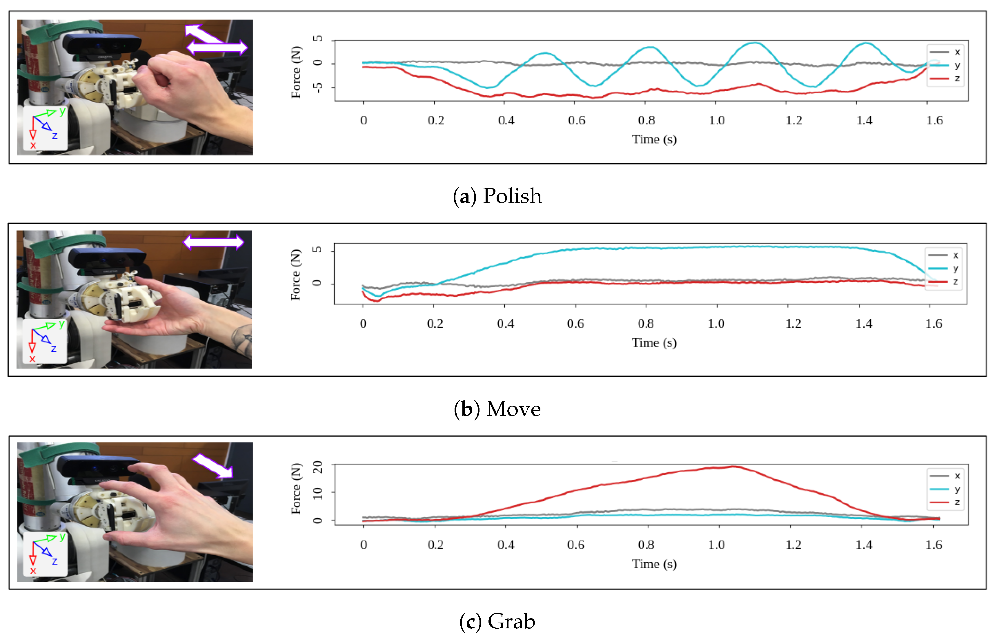
Since it was expected to be easier to classify, the mechanical dataset only contained 600 samples. Recall that we had three classes, and we used two users; thus, each user performed 100 samples of each class. The physical contact was always done following restricted patterns for each intention/class. Figure 3 depicts both, the different axes in which the operator was supposed to apply the force and the corresponding force signals we detected using the sensor. For the polishing intention, we moved periodically only in the axis Y, and we pushed towards the robot, the negative Z-axis (Figure 3a). In order to move the robot, we moved just in one direction for each sample and only in the Y-axis (Figure 3b). Finally, to grab the object, we pulled the robot’s end-effector towards ourselves, the positive Z-axis (Figure 3c).
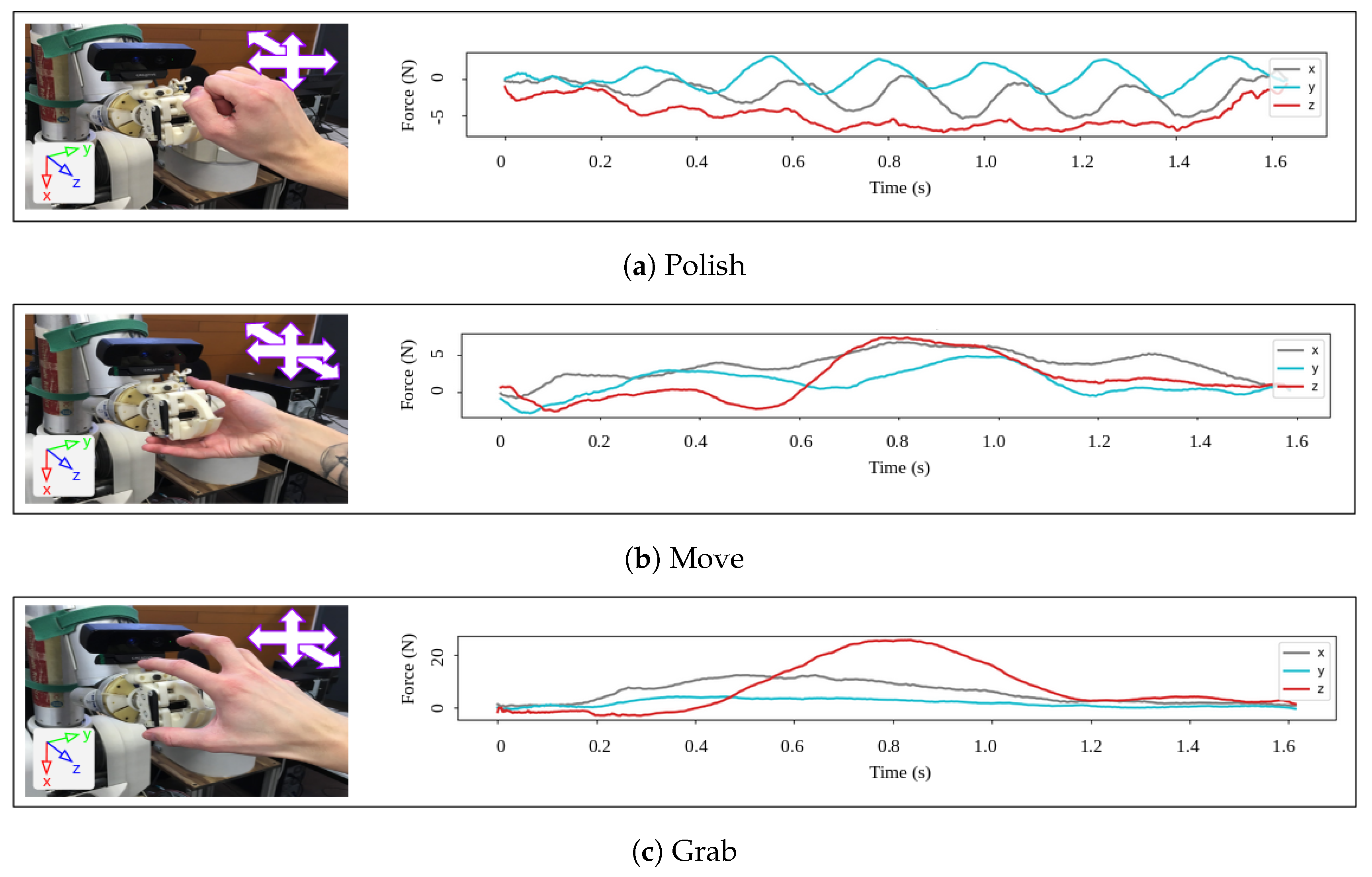
Unlike with the mechanical dataset, the natural dataset contained more samples, 900. Recall that we had three classes, and we used two users; thus, each user performed 150 samples of each class. In this case, the physical contact for each intention/class could be done following several natural patterns, which increased the ambiguity between classes. In Figure 4, it is possible to see the different axes in which the operator was supposed to apply the force and the corresponding force signals we detected using the sensor. For instance, the intention of polishing could now be done by describing circles and also using the X-axis (Figure 4a). The patterns to move the robot now included any of the directions of the three spatial axes (Figure 4b). Finally, the operator could now try to grab the object pulling, but not only towards the exact direction of the Z-axis (Figure 4c).
It is worth discussing the visual differences between the signals of both datasets. In the mechanical dataset, signal forces looked different when we considered the entire time series, but also after 0.4 s of signals. Forces occurred in isolated axes for each of the operator’s actions/intents, and ambiguity between classes was kept to a minimum. Hence, it was possible to discriminate between classes with a reduced amount of force information. This was not the case for the natural dataset. Of course, signals from different classes were still distinct if we considered the whole temporal sequence. Nevertheless, unlike with the mechanical dataset, we could not be so sure about the label of each of the signals after only 0.4 s. Please, recall that, although for illustrative purposes, the figures only show the linear forces, our classification process used both torque and linear signals. Together with the dataset, we also provide some Python code to run our proposed approaches and use the data (http://doi.org/10.5281/zenodo.3522205). Therefore, other people can learn how to use the dataset on their own.

4. Force Based Operator’s Intention Inference

In order to infer humans’ intents, we have evaluated the performance of two approaches using the natural dataset. We compared them and chose one, which was used during the validation carried out in Section 5. Finally, the chosen approach was also used to analyze the differences between the natural and mechanic datasets. These results are part of the experimental findings presented in our work. One of the approaches, kNN + DTW, was based on a classifier that directly used the raw sensor data to perform the inference, whereas the other one, GPLVM + SVM, used a lower dimensional representation of the data. Recall that we sought a natural human–robot interaction, a fast reaction of the robot, and if possible, an approach that dealt with heterogeneous industrial contextual data.

4.1. Evaluation Setup for the Proposed Approaches

The performance of the proposed approaches was evaluated following the considerations explained in this section. Cross-validation without replacement was applied ten times, and the data were randomly split into training (75%) and test (25%) sets. The chosen metric to evaluate the performance was the F1-score, which captures both the precision and the recall of the test.
In order to fulfill the requirement of a profitable robot reaction, the prediction time should be short enough so that the proposed methods apply to our realistic scenario. For that reason, we did not consider all the samples, but smaller portions of them (windows), which contained only their initial information. In total, five different window’s sizes were evaluated: 0.1, 0.2, 0.5, 0.7, and 1 s (see Figure 5). The intuition is that the larger the sampling window, the higher would be the chances to classify the human’s intention properly, but the longer the operator would need to wait until the robot reacts to the interaction. Therefore, we aimed to find a trade-off between the prediction time and the classification performance. Our experience said that 1 s was a convenient amount of prediction time for an efficient and feasible human–robot collaboration. Thus, longer inference time would be undesirable. Note that the total prediction time would include both the sampling window’s size and the time the approach needs to infer the label of the sample.

4.2. Raw Data Based Classification

In this approach, using the data obtained from the sensor directly, the classification was done utilizing a k-Nearest Neighbors (kNN) classifier with Dynamic Time Warping (DTW) [30] as the metric. In particular, we used k = 1 . While being a simple method, 1NN + DTW’s performance seems to be hard to beat by other approaches in time series classification problems [31].

4.2.1. Implementation Details of the Raw Data Based Classification

Dynamic time warping is a time dependent algorithm used to measure similarity between two temporal sequences that may vary in speed. For instance, similarities in polishing could be detected using DTW, even if the operator polishes faster or slower than on other occasions. DTW is a computationally-intense technique, with quadratic time and memory complexity. However, there are some ways to accelerate computation. In our case, we used the library Fast DTW [32]. DTW is meant to be utilized for univariate time series, which was not our case since we had six sensor axes. From the literature, we know at least two obvious approaches to tackle this and generalize DTW for multi-dimensional time series: dependent and independent DTW (see Figure 6) [33]. The kNN classifier was taken from the scikit learn library [34]. Since default implementations of both kNN and Fast DTW do not allow working with multi-dimensional time series, it was necessary to adapt the libraries we used. Apart from those modifications, we used the values set by default.

4.2.2. Evaluation of the Raw Data Based Classification

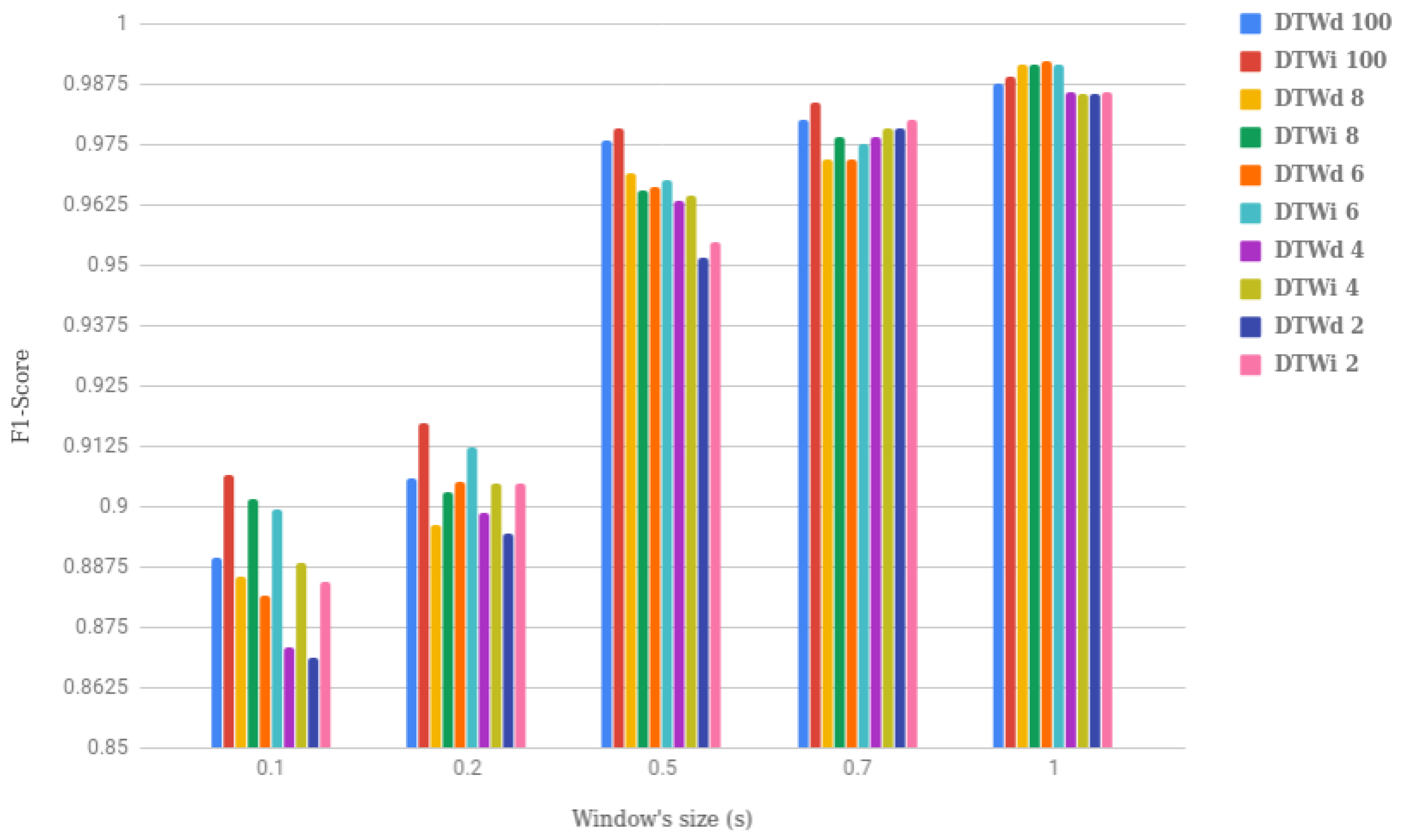
The proposed method, 1NN + DTW, was evaluated for each of the window sizes previously defined, concerning the classification performance and the inference time per sample. Recall that two different implementations of multi-variate DTW were used, dependent and independent, DTWd and DTWi, respectively. Due to the lazy learning nature of the kNN classifier, we also evaluated how the length of the samples fed to the classifier affected the inference time. In particular, we sub-sampled the measurements of the windows to smaller portions. We considered five different lengths, which were expressed as the percentage of the window’s length that remained after the sub-sampling: 100% (no sub-sampling), 8%, 6%, 4%, and 2%. Figure 7 and Figure 8 show the results of the evaluation.
There are many conclusions that could be drawn by analyzing the information shown in Figure 7 and Figure 8. In the first place, the bigger the window, the better the performance; see the evolution of F1-score in Figure 7. It is also true that the growth of the window’s size resulted in an increment of the inference time per sample (see Figure 8). This is reasonable since the kNN algorithm is a lazy learner. Any time a new sample is to be classified, the similarity between that sample and the rest of the training samples is computed. Hence, the longer the samples, the more time it takes to compute the similarity, prolonging the whole inference process.
The best F1-score result (99.24%) was obtained for the case of using DTWd with the window size of one second and sub-sampling of 6% of the total window’s size (see the orange bar in Figure 7). The inference time per sample for this same case was above half a second (0.7 s), which can be seen looking at the same bar in Figure 8. Therefore, the total operator’s intent inference time would be around 1.7 s, which is above the one second we sought, so this was not a valid alternative.
Fortunately, reducing the window’s size, while helping to reduce the inference time, did not decrement the performance too much. As can be seen in Figure 7, from windows bigger than 0.5 s, the value of the F1-score was always above 95%. The best F1-score value for that window was around 97.5%, which was a really good result. It corresponded to the case of using all the data within the window’s size together with DTWi (red bar). Nevertheless, if we used that configuration for the approach, the time needed to infer the operator’s intent would be above seven seconds, once again undesirable.
We needed to find the most convenient combination of: the DTW version, sampling window size, and whether sub-sampling was needed or not. Indubitably, we discarded the case in which sub-sampling was not applied, since the inference time (blue and red bars in Figure 8) was always above the desired one. Any case that used the one second window could also be dismissed, since the performance was not much better than for the case of using 0.5 or 0.7 s windows. Hence, we focused on the 0.5 and 0.7 s windows, in which there was not any combination that, at the same time, performed better and faster than the rest. Nonetheless, should we choose one case, we would select a case in which the trade-off between inference time (0.8 s) and performance (97.99%) was rather good. This case corresponded to DTWi, a window of 0.7 s, and sub-sampling of the data to 2% of the window’s size (pink bar in Figure 7).

4.3. Feature Based Classification

In this section, we propose a twofold machine learning approach to infer the human operator’s intentions. First, we reduced the dimensionality of the data using an unsupervised method: Gaussian Process Latent Variable Model (GPLVM) [35]. Then, we used a Support Vector Machine (SVM) classifier, which was trained using the lower dimensional representation of the data. GPLVM is a non-linear dimensionality reduction method that can be considered as a multiple-output GP regression model where only the output data are given. The inputs are unobserved and treated as latent variables; however, instead of integrating out the latent variables, they are optimized. By doing this, the model gets more tractable, and some theoretical grounding for the approach is given by the fact that the model can be seen as a non-linear extension of the linear Probabilistic PCA (PPCA) [36]. Note that in this case, the temporal sequences are just considered as long feature vectors, so that the temporal relation between subsequent signal measurements is not explicitly considered. However, dimensionality reduction has proven to be an effective technique in time series analysis, in which data are remarkably high dimensional [37,38,39].

4.3.1. Implementation Details of the Feature Based Classification

The implementation of the proposed method, GPLVM + SVM, relied on two existing libraries: the GPy library [40] for the dimensionality reduction and the scikit learn library for the SVM classifier [41]. In the case of the latter, we used the default values for all the parameters. However, concerning GPLVM, it was necessary to set some parameters: kernel, optimizer, and the maximum number of optimization steps. Firstly, we chose a kernel that was a combination of the Radial Basis Function (RBF) kernel together with a bias kernel. The RBF kernel was selected because it is one of the most well known kernels for non-linear problems. We added the bias kernel to enable the kernel function to be computed not only in the origin of coordinates. Secondly, for the optimization process, we used one of the optimizers already implemented in GPy, limited-memory Broyden–Fletcher–Goldfarb–Shannon (BFGS) [42]. We chose this optimizer because, unlike others included in the library, it was quite stable concerning the number of optimization steps needed to converge. Finally, the maximum number of optimization steps was set to 5000, which in most cases was enough for the optimization to converge.
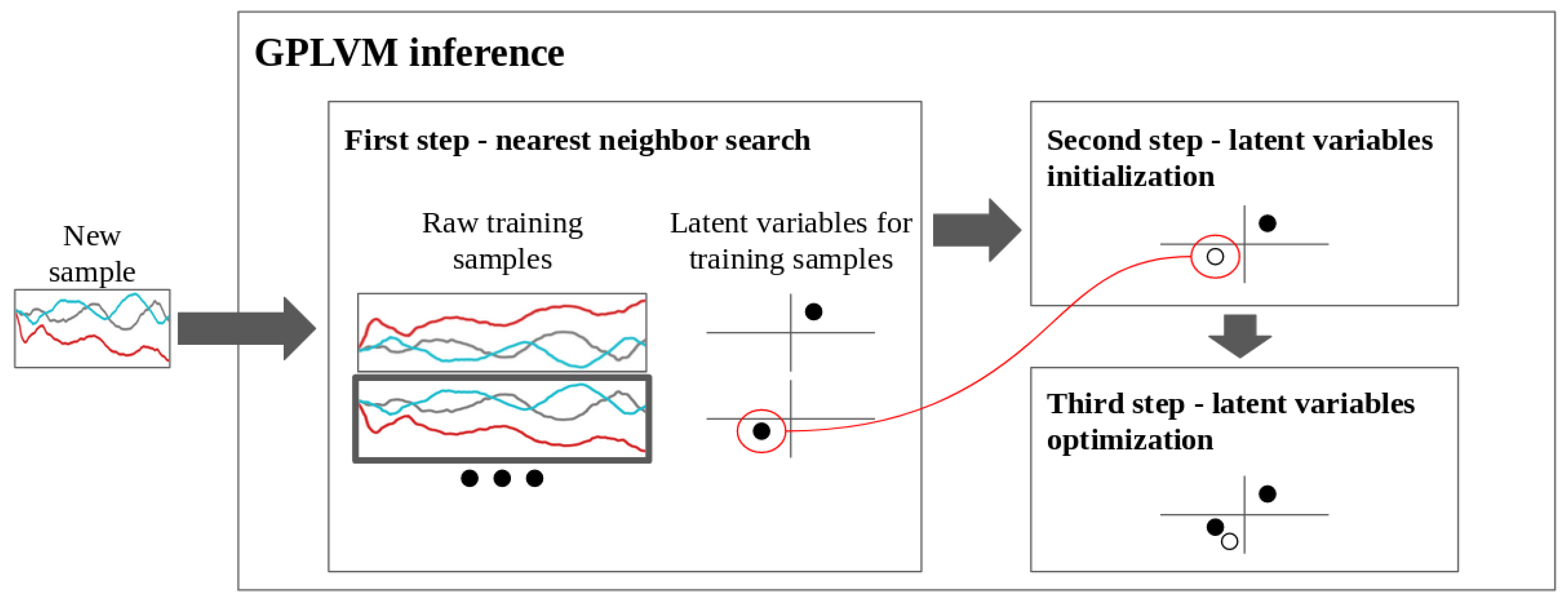
The implementation of the GPLVM algorithm allowed us to use two different types of latent variable inference: with the optimization step (GPLVM-op) and without the optimization step (GPLVM). For us, the most relevant difference between them was that the inference with optimization took more time, but it would be more correct in theory and would lead to more accurate results. Nevertheless, as we will see in Section 4.3.2, the inference with optimization did not always ensure better performance. Once an already optimized GPLVM received a new sample to infer its latent variables, the global inference process was divided into three steps. The first step, nearest neighbor search, was focused on finding which of the training samples was the most similar to the new sample. This was done by computing the similarity between the new sample and all the training samples employing the Euclidean distance. The second step, latent variables’ initialization, consisted of setting the value of the inferred latent variables to the values of the latent variables of the nearest neighbor found in the previous step. Finally, during the third step, latent variables’ optimization, the value of the initialized latent variables was refined through optimization. Figure 9 depicts the global pipeline of the inference process detailed above.

4.3.2. Evaluation of the Feature Based Classification

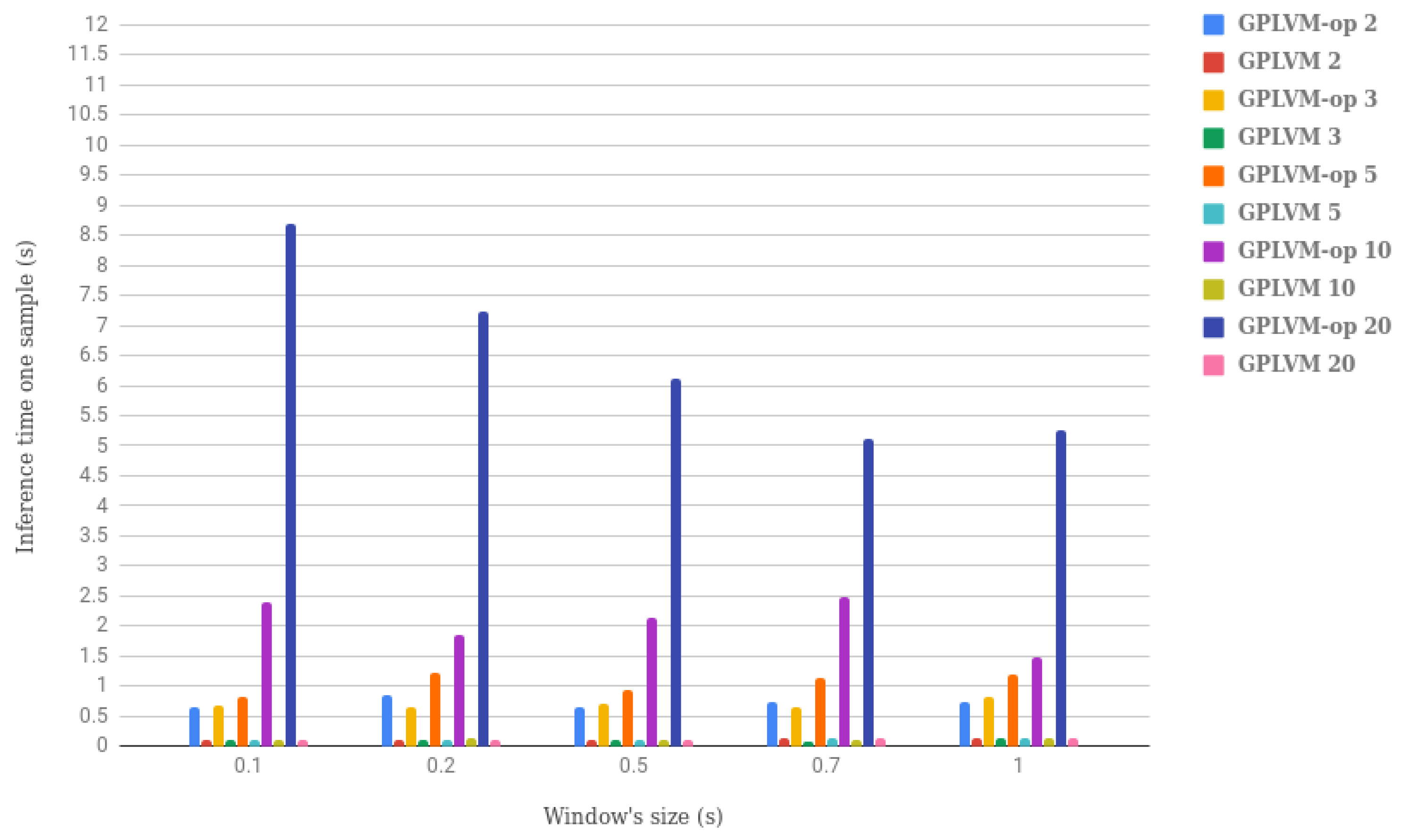
The proposed method, GPLVM + SVM, was evaluated for all the different already mentioned window sizes about both the classification performance and the inference time per sample. A priori, we did not know which size of the latent space would produce a good performance. Therefore, different sizes of latent space were also evaluated: 2, 3, 5, 10, and 20 latent variables. Besides, the two types of GPLVM were evaluated as well: optimized (GPLVM-op) and non-optimized (GPLVM). Figure 9 depicts the global modular structure of the GPLVM inference process. Figure 10 and Figure 11 show respectively the results of both the F1-score and the inference time with respect to the different window sizes and the GPLVM methods used.
Evaluating in detail the results depicted in such figures, probably, the most evident conclusion is the effect of the optimization during the inference step in the GPLVM. The inference time per sample was always longer when GPLVM inference was optimized. Indeed, that time grew accordingly to the number of latent variables (see Figure 11). Another interesting finding was that the inference time per sample, when there was no optimization, remained quite short and stable no matter the window’s size nor the number of latent variables (see Figure 11). Hence, in terms of inference time, GPLVM without optimization was preferred. Moreover, as can be seen in Figure 10, the performance score between both optimized and not optimized versions was negligible. This fact reinforced the previous result, allowing us to conclude that the non-optimized version of GPLVM was the most convenient alternative.
Focusing on Figure 10, it is observable that the more latent variables we used, the better was the result. Specifically, for the cases in which we used two and three latent variables (specially two), the performance (F1-score) was usually much poorer. The best result in terms of performance, an F1-score of 99.33%, corresponded to the GPLVM version without optimization, the window of 1 s, and 20 latent variables. The inference time per sample was around 0.15 s, so the total inference time was 1.15 s, slightly superior to the one second we set as desirable. Thus, we decided to reduce the window’s size to 0.7 s. In this case, the best alternative was to use 10 latent variables and, again, the non-optimized GPLVM. This resulted in losing a bit of quality in the performance, from 99.33% to 98.14%, not noteworthy, but decreasing the time from 1.15 to 0.85 s, fulfilling our requirements.

4.4. Raw Data Based vs. Feature Based Classification

In this section, we compare only the best combination of parameters for each of the two studied methods. Finally, we selected one of them to be used during the experimental validation proposed in Section 5. Recall that at the beginning of this work, we stated some requirements that the selected approach should fulfill. The human and the robot should interact naturally, and the robot adaptation should last one second at most. Furthermore, in the future, we aim to consider the contextual information of the industrial processes surrounding the proposed collaborative task. Hence, it would be desirable that the method to infer the human’s intention could deal with heterogeneous data, not only temporal sequences.
The selected combination in the case of 1NN + DTW ensured an inference time of 0.8 s and a performance score of 97.99%, which was rather good. It corresponded to using independent DTW, a window of 0.7 s, and sub-sampling of the data to 2% of the window’s size (see Section 4.2.2 for more detail). When using GPLVM + SVM, the selection was GPLVM without optimization, a window of 0.7 s, and 10 latent variables. This approach resulted in an F1-score of 98.14% and an inference time of 0.85 s (see Section 4.3.2 for more detail). As we can see, the quantitative differences between the two alternatives were negligible. Therefore, to provide more useful insights into the comparison between 1NN + DTW and GPLVM + SVM, we analyzed them using more qualitative measures. They were extracted from the hands-on experience acquired along the developed work and were meant to ease the selection procedure.
  • Ease of implementation: Both methods were relatively simple to implement and use. Conceptually and algorithmically, 1NN + DTW was a simple machine learning technique; only the versions of DTW for multivariate data presented a bit of difficulty. GPLVM was theoretically more complex, and reaching a profound understanding of the mathematical background of this technique would require effort. However, the GPy library eased the use of GPLVM without the need to dig too much into the theoretical details.
  • Data visualization: GPLVM allowed us to project the sequential data samples into just a few latent variables and then visualize the data distribution in either 2D or 3D. This can be useful to analyze the dataset easily, and it was something that could not be done using 1NN + DTW.
  • Generalization to other scenarios: This aspect is rather important for us because in the future, we would like to include heterogeneous environmental variables in the learning pipeline. Examples of contextual variables are: if the grasped object is heavy or not and if the user is inside the workspace or not. In this case, these two variables are binary and could be added to the feature vector of each sample to learn some environmental aspects related to safety. GPLVM could be used to reduce the dimensionality of temporal sequences to just a few features. Then, other contextual variables could be concatenated to the resulted feature vector, and SVM would be used to learn not only the physical interactions but also the contextual information. 1NN + DTW, however, cannot deal with other data apart from sequential. It would be necessary to use a second kNN model with another metric (e.g., Euclidean) and then apply ensemble learning techniques.
Based on the previous analysis, we selected GPLVM + SVM. In particular, we proposed to use GPLVM without optimization during the inference, a sampling window of 0.7 s, and 10 latent variables. The first reason was that we thought GPLVM’s generalization capabilities could help us in future works. In robotics, especially in industrial environments, data are presented in heterogeneous ways: sequential data, digital, etc. Let us consider one of the examples proposed in the generalization paragraph. If the object the robot grasps is too heavy, we could just add a “1” to the feature vector of latent variables and train the SVM classifier with the new extended vector. Therefore, it could be learned that even when the inferred human’s intention is grabbing the object, the robot must never open the gripper if the object is too heavy. Of course, if we consider only one environmental variable, the easiest way to tackle this event would be to add a conditional statement to the control code of the robot. However, if the number of those variables increases, machine learning methods could help. Furthermore, GPLVM allowed us to visualize the distribution of the data we worked with, which could be especially useful if the dataset were enlarged by other people, and we wanted to see how the different datasets related to each other.

4.5. Comparison of Natural and Mechanical Datasets

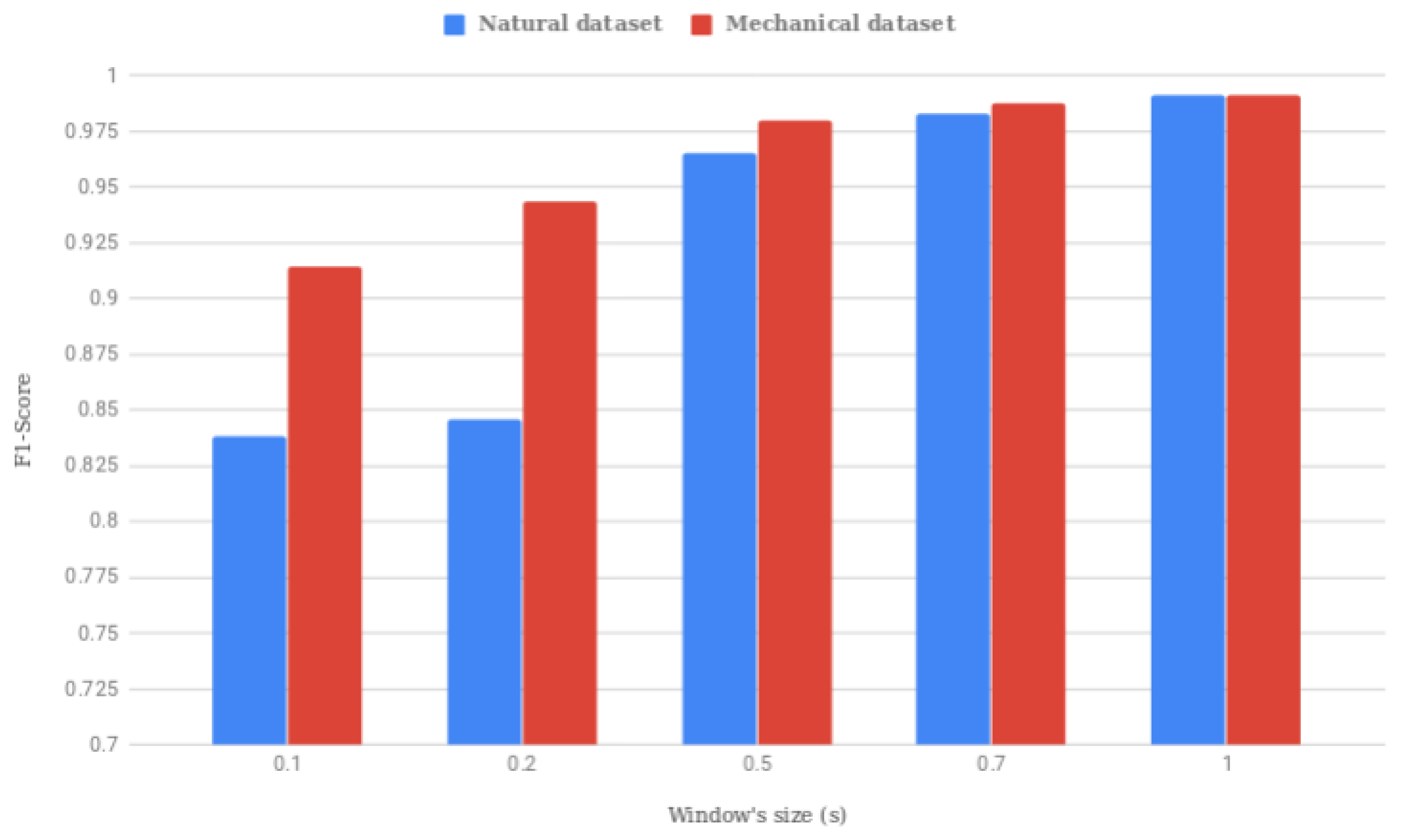
In this section, we evaluate and compare the performance of the chosen approach, GPLVM + SVM, using both datasets, the natural and the mechanical. We assumed that the mechanical dataset would show a good performance even with a small sampling window sizes. Given that, we wanted to analyze if the proposed method, for the sampling window of 0.7 s, could work similarly well, not only with the mechanical, but also with the natural dataset. Recall that we chose to use the non-optimized GPLVM inference and 10 latent variables. Although the selected sampling window’s size was 0.7, during this section, we tested the approach against the usual five sizes we used along the rest of the document. As was done previously, we used cross-validation without replacement ten times, and the data were randomly split into training (75%) and test (25%) sets.
Figure 12 depicts the F1-score values obtained from the evaluation of GPLVM + SVM against both datasets. This bar diagram shows that indeed, our previous assumption was true. In general, using the mechanical dataset, we obtained better results than with the natural data. Specifically, when the window’s size was 0.2 s, the F1-score was even close to 95%. However, we also observed that for the window chosen for our validation with users, 0.7 s, the differences between the performance using any of the datasets were minimal. Therefore, the proposed approach worked quite well even when the dataset contained more natural samples of physical human–robot interaction.

5. Validation: Inferring Operator’s Intent in a Realistic Scenario

To validate the selected approach, GPLVM + SVM, we set up an experiment in which several users individually collaborated with a robotic arm according to the industrial scenario of polishing car emblems. The validation was conducted using fifteen healthy individuals within an age range of 18 to 35. Users were selected among people who had knowledge about the robotics domain and had been in contact with robots before. We did not include people with reduced mobility or any cognitive disability, which could affect the perception of the robot’s behavior, endangering the users’ integrity. Each of the users received an individual explanation, no more than five minutes, about how they were expected to interact with the robot. This included both general information about the system and particular notions about the expected movements for each of the three classes/intentions. Nevertheless, the users were not allowed to train before the evaluation began, because we wanted to evaluate if there was an adaptation of the user to how the system inferred the different intentions. Users were also informed about their rights, possible risks, and were asked to sign an ethical approval specifically designed for this experiment. Note that we followed CSIC (Spanish National Research Council) ethical procedures and asked for ethical consent from the Human Subject Research Committee of CSIC before the validation was conducted.
Recall that the parameter combination for the chosen approach was: GPLVM without optimization, a sampling window of 0.7 s, and 10 latent variables. In this section, we give the flavor of the validation setup, and we evaluate and discuss the obtained results.

5.1. Setup

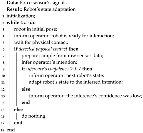
The validation setup was aimed at fulfilling the needs required by a human and a robot to collaborate on an industrial task in which the force exchange is not only present, but fundamental for the accomplishment of the task. Using the force based information, the robot should be able to identify the intent of the operator (Section 3.2) and to adapt its state/behavior to it. In order to provide a bi-directional communication, we equipped the robot with a force sensor, used to measure the interaction from the human to the robot, and an armband made of LEDs through which the robot informed the user of its internal state. The latter allowed us to display different patterns (see Figure 13). The finite state machine of the control of robot during the validation experiment is shown in Algorithm 1.
Algorithm 1: Finite state machine of the control of the robot during the validation.
Electronics 08 01306 i001
Recall that this scenario was inspired by a real industrial case in which an operator was meant to inspect and polish car emblems. Please refer to Figure 2a to see the different parts of the robot setup used. We can only show the adapter where the emblem is attached since emblems contain private commercial brand logos and cannot be shown due to confidentiality agreements. Another important aspect related to the setup is how the user is located with respect to the robot. We chose to pose the operator in front of the robot so that the physical interaction was comfortable. During the experiment, the operator will have a rag that would be used to polish. Figure 2b shows an example of the pose of a user while polishing. A video of the validation with users can be found at www.iri.upc.edu/groups/perception/SIMBIOTS.

5.2. Evaluation

Each user was asked to perform thirty trials randomly selected from the three operator’s intent/actions explained in Section 3.2. We made sure that among the thirty trials, ten corresponded to each of the three classes/intentions. Note that since trials were randomly arranged for each person, there could not be any bias in our evaluation due to the order of the trials. Both the ground truth and the inferred value were annotated for each user’s trial. In this section, we analyze the overall performance of the system (confusion matrix) and the overall adaptation of the users throughout the experimental validation.
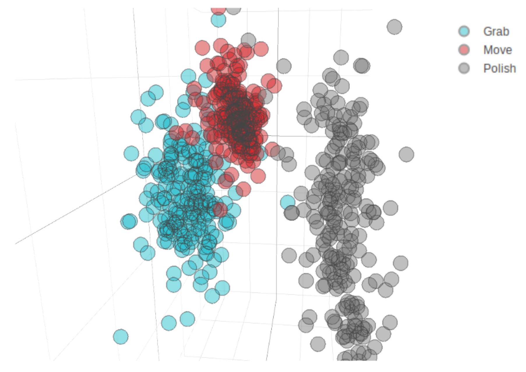
A confusion matrix of the performance of the system for each user was computed, then we calculated the final mean confusion matrix shown in Figure 14, which contained the average result for all users. The most obvious observation one can make is that the “move” intent was the easiest to identify. Indeed, the confusion matrix was not symmetric, and this class showed a large percentage of false positives, which was a symptom of a clear bias of the model in favor of this class. This can be better understood by looking at Figure 15. This figure shows the sample distribution in the three-dimensional space defined by the most significant/discriminating latent variables among the ten used. We can observe how the samples from the “move” class fell in the middle of the other two classes, which explains why there were many false positives, shared with the other two classes. However, given the bias in favor of this class and the higher proximity to the “grab” class, this latter was the class with the biggest number of false positives.
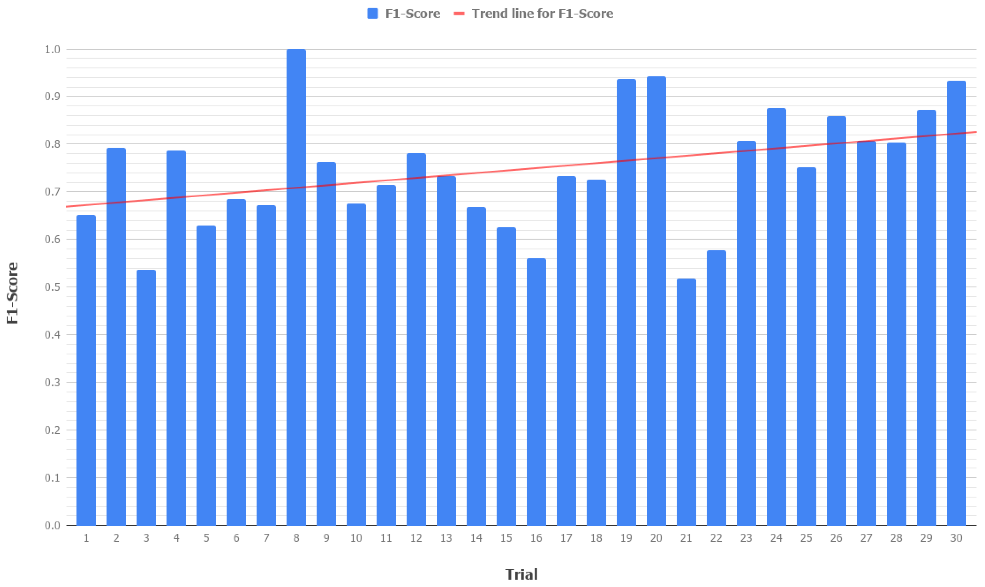
As stated before, we also studied if there was an adaptation of the users to the system, which would be observable in the performance of the system along the validation experiments. Recall that users only received a short explanation of the three classes and in which axes they could perform the movements for each action. There was ambiguity among classes, and users had a particular way to move for each action. Because of this, during the first trials, the system’s performance was poorer. When we talk of adaptation, we mean that the users understand which movements for each class ensure a better performance of the system. Note that this is possible because users could see the result of the inference.
We computed the average performance of the system for all the trials and users, and the result showed a positive slope of the trend line for the F1-score (Figure 16). We considered that once the trend line was above 0.8, users had already adapted. In our case, this corresponded to the last five trials of the experiment.

6. Conclusions

In this article, we presented our work on inferring operators’ intent throughout the execution of an industrial collaborative task in which a robot and an operator exchanged forces while sharing the accomplishment of the task. This work consisted of three major contributions: (a) force based operator’s intention inference; (b) force based dataset of physical human–robot interaction; and (c) validation of the whole system in a scenario inspired by a realistic industrial application. In our work, the physical interaction between the robot and the human not only existed, but also played a major role since it was the main source of information for the robot to infer the human’s intent. Were humans and robots to collaborate in industrial environments in the factories of the future, the main interaction would be physical. Hence, our work means a step forward to enhance humans’ and robots’ collaboration in real case studies with more natural and user-friendly interaction. In the future, we will consider exploring other model based representations of the inherent contextual knowledge of collaborative shared tasks, to extend our current system to a wider range of more complicated scenarios.

Author Contributions

Data curation, A.O.-A.; software, A.O.-A.; supervision, S.F. and G.A.; Writing—review & editing, A.O.-A., S.F. and G.A.

Funding

This work is supported by the Regional Catalan Agency ACCIÓthrough the RIS3CAT2016 project SIMBIOTS(COMRDI16-1-0017) and the Spanish State Research Agency through the María de Maeztu Seal of Excellence to IRI (Institut de Robòtica i Informàtica Industrial)(MDM-2016-0656) and the HuMoUR project TIN2017-90086-R (AEI/FEDER, UE).

Acknowledgments

Firstly, this work was possible thanks to the help of the users that were part of the validation phase, so we thank all of them for their contribution. We cannot forget the help provided by Marc Maceira, who was fundamental throughout the dataset gathering and also during the experiment with users.

Conflicts of Interest

The authors declare no conflict of interest.

References

  1. Michalos, G.; Makris, S.; Tsarouchi, P.; Guasch, T.; Kontovrakis, D.; Chryssolouris, G. Design considerations for safe human–robot collaborative workplaces. Procedia CIRP 2015, 37, 248–253. [Google Scholar] [CrossRef]
  2. Villani, V.; Pini, F.; Leali, F.; Secchi, C. Survey on human–robot collaboration in industrial settings: Safety, intuitive interfaces and applications. Mechatronics 2018, 55, 248–266. [Google Scholar] [CrossRef]
  3. Michalos, G.; Makris, S.; Spiliotopoulos, J.; Misios, I.; Tsarouchi, P.; Chryssolouris, G. ROBO-PARTNER: Seamless human–robot cooperation for intelligent, flexible and safe operations in the assembly factories of the future. Procedia CIRP 2014, 23, 71–76. [Google Scholar] [CrossRef]
  4. Tsarouchi, P.; Michalos, G.; Makris, S.; Athanasatos, T.; Dimoulas, K.; Chryssolouris, G. On a human–robot workplace design and task allocation system. Int. J. Comput. Integr. Manuf. 2017, 30, 1272–1279. [Google Scholar] [CrossRef]
  5. Wang, L.; Gao, R.; Váncza, J.; Krüger, J.; Wang, X.V.; Makris, S.; Chryssolouris, G. Symbiotic human–robot collaborative assembly. CIRP Ann. 2019, 68, 701–726. [Google Scholar] [CrossRef]
  6. Roy, S.; Edan, Y. Investigating joint-action in short-cycle repetitive handover tasks: The role of giver versus receiver and its implications for human–robot collaborative system design. Int. J. Soc. Robot. 2018, 1–16. [Google Scholar] [CrossRef]
  7. Someshwar, R.; Edan, Y. Givers & receivers perceive handover tasks differently: Implications for human–robot collaborative system design. arXiv 2017, arXiv:1708.06207. [Google Scholar]
  8. Bauer, W.; Bender, M.; Braun, M.; Rally, P.; Scholtz, O. Lightweight Robots in Manual Assembly—Best to Start Simply. Examining Companies’ Initial Experiences with Lightweight Robots; Fraunhofer IAO: Stuttgart, Germany, 2016. [Google Scholar]
  9. Someshwar, R.; Meyer, J.; Edan, Y. A timing control model for hr synchronization. IFAC Proc. Vol. 2012, 45, 698–703. [Google Scholar] [CrossRef]
  10. Someshwar, R.; Kerner, Y. Optimization of waiting time in HR coordination. In Proceedings of the 2013 IEEE International Conference on Systems, Man, and Cybernetics, Manchester, UK, 13–16 October 2013; IEEE: Piscataway, NJ, USA, 2013; pp. 1918–1923. [Google Scholar]
  11. Cherubini, A.; Passama, R.; Crosnier, A.; Lasnier, A.; Fraisse, P. Collaborative manufacturing with physical human–robot interaction. Robot. Comput. Integr. Manuf. 2016, 40, 1–13. [Google Scholar] [CrossRef]
  12. Maurtua, I.; Ibarguren, A.; Kildal, J.; Susperregi, L.; Sierra, B. Human–robot collaboration in industrial applications: Safety, interaction and trust. Int. J. Adv. Robot. Syst. 2017, 14. [Google Scholar] [CrossRef]
  13. de Gea Fernández, J.; Mronga, D.; Günther, M.; Wirkus, M.; Schröer, M.; Stiene, S.; Kirchner, E.; Bargsten, V.; Bänziger, T.; Teiwes, J.; et al. iMRK: Demonstrator for Intelligent and Intuitive Human–Robot Collaboration in Industrial Manufacturing. KI-Künstliche Intell. 2017, 31, 203–207. [Google Scholar] [CrossRef]
  14. Raiola, G.; Restrepo, S.S.; Chevalier, P.; Rodriguez-Ayerbe, P.; Lamy, X.; Tliba, S.; Stulp, F. Co-manipulation with a library of virtual guiding fixtures. Auton. Robot. 2018, 42, 1037–1051. [Google Scholar] [CrossRef]
  15. Munzer, T.; Toussaint, M.; Lopes, M. Efficient behavior learning in human–robot collaboration. Auton. Robot. 2018, 42, 1103–1115. [Google Scholar] [CrossRef]
  16. Peternel, L.; Tsagarakis, N.; Caldwell, D.; Ajoudani, A. Robot adaptation to human physical fatigue in human–robot co-manipulation. Autonomous Robots 2018, 42, 1011–1021. [Google Scholar] [CrossRef]
  17. Rozo, L.; Calinon, S.; Caldwell, D.G.; Jimenez, P.; Torras, C. Learning physical collaborative robot behaviors from human demonstrations. IEEE Trans. Robot. 2016, 32, 513–527. [Google Scholar] [CrossRef]
  18. Mazhar, O.; Ramdani, S.; Navarro, B.; Passama, R.; Cherubini, A. Towards real-time physical human–robot interaction using skeleton information and hand gestures. In Proceedings of the 2018 IEEE/RSJ International Conference on Intelligent Robots and Systems (IROS), Madrid, Spain, 1–5 October 2018; IEEE: Piscataway, NJ, USA, 2018; pp. 1–6. [Google Scholar]
  19. Zhao, R.; Drouot, A.; Ratchev, S. Classification of Contact Forces in Human-Robot Collaborative Manufacturing Environments. SAE Int. J. Mater. Manuf. 2018, 11, 5–10. [Google Scholar] [CrossRef]
  20. Gaz, C.; Magrini, E.; De Luca, A. A model based residual approach for human–robot collaboration during manual polishing operations. Mechatronics 2018, 55, 234–247. [Google Scholar] [CrossRef]
  21. Losey, D.P.; McDonald, C.G.; Battaglia, E.; O’Malley, M.K. A review of intent detection, arbitration, and communication aspects of shared control for physical human–robot interaction. Appl. Mech. Rev. 2018, 70, 010804. [Google Scholar] [CrossRef]
  22. Mohammad, Y.; Xu, Y.; Matsumura, K.; Nishida, T. The H3R explanation corpus human-human and base human–robot interaction dataset. In Proceedings of the 2008 International Conference on Intelligent Sensors, Sensor Networks and Information Processing, Sydney, NSW, Australia, 15–18 December 2008; IEEE: Piscataway, NJ, USA, 2008; pp. 201–206. [Google Scholar]
  23. Jayagopi, D.B.; Sheikhi, S.; Klotz, D.; Wienke, J.; Odobez, J.M.; Wrede, S.; Khalidov, V.; Nguyen, L.; Wrede, B.; Gatica-Perez, D. The Vernissage Corpus: A Multimodal Human-Robot-Interaction Dataset; Technical Report; Idiap Research Institute: Martign, Switzerland, 2012. [Google Scholar]
  24. Bastianelli, E.; Castellucci, G.; Croce, D.; Iocchi, L.; Basili, R.; Nardi, D. HuRIC: A Human Robot Interaction Corpus. In Proceedings of the Ninth International Conference on Language Resources and Evaluation, Reykjavik, Iceland, 26–31 May 2014; European Language Resources Association: Paris, France, 2014; pp. 4519–4526. [Google Scholar]
  25. Lemaignan, S.; Kennedy, J.; Baxter, P.; Belpaeme, T. Towards “machine-learnable” child-robot interactions: The PInSoRo dataset. In Proceedings of the IEEE Ro-Man 2016 Workshop on Long-Term Child-Robot Interaction, New York, NY, USA, 31 August 2016. [Google Scholar]
  26. Celiktutan, O.; Skordos, E.; Gunes, H. Multimodal human-human–robot interactions (mhhri) dataset for studying personality and engagement. IEEE Trans. Affect. Comput. 2017. [Google Scholar] [CrossRef]
  27. Yu, K.T.; Bauza, M.; Fazeli, N.; Rodriguez, A. More than a million ways to be pushed. A high-fidelity experimental dataset of planar pushing. In Proceedings of the 2016 IEEE/RSJ International Conference on Intelligent Robots and Systems (IROS), Daejeon, Korea, 9–14 October 2016; IEEE: Piscataway, NJ, USA, 2016; pp. 30–37. [Google Scholar] [Green Version]
  28. De Magistris, G.; Munawar, A.; Pham, T.H.; Inoue, T.; Vinayavekhin, P.; Tachibana, R. Experimental Force-Torque Dataset for Robot Learning of Multi-Shape Insertion. arXiv 2018, arXiv:1807.06749. [Google Scholar]
  29. Huang, Y.; Sun, Y. A Dataset of Daily Interactive Manipulation. arXiv 2018, arXiv:1807.00858. [Google Scholar] [CrossRef]
  30. Berndt, D.J.; Clifford, J. Using dynamic time warping to find patterns in time series. In Proceedings of the 3rd International Conference on KDD Workshop, Seattle, WA, USA, 31 July–1 August 1994; AAAI: Menlo Park, CA, USA; Volume 10, pp. 359–370. [Google Scholar]
  31. Bagnall, A.; Bostrom, A.; Large, J.; Lines, J. The great time series classification bake off: An experimental evaluation of recently proposed algorithms. Extended version. arXiv 2016, arXiv:1602.01711. [Google Scholar]
  32. Salvador, S.; Chan, P. Toward accurate dynamic time warping in linear time and space. Intell. Data Anal. 2007, 11, 561–580. [Google Scholar] [CrossRef] [Green Version]
  33. Shokoohi-Yekta, M.; Hu, B.; Jin, H.; Wang, J.; Keogh, E. Generalizing DTW to the multi-dimensional case requires an adaptive approach. Data Min. Knowl. Discov. 2017, 31, 1–31. [Google Scholar] [CrossRef]
  34. k-Nearest Neighbors Classifier (Scikit-Learn). Available online: https://scikit-learn.org/stable/modules/generated/sklearn.neighbors.KNeighborsClassifier (accessed on 1 November 2019).
  35. Lawrence, N.D. Gaussian process latent variable models for visualization of high dimensional data. In Advances in Neural Information Processing Systems; MIT Press: Boston, MA, USA, 2004; pp. 329–336. [Google Scholar]
  36. Tipping, M.E.; Bishop, C.M. Probabilistic principal component analysis. J. R. Stat. Soc. Ser. B Stat. Methodol. 1999, 61, 611–622. [Google Scholar] [CrossRef]
  37. Su, B.; Ding, X.; Wang, H.; Wu, Y. Discriminative dimensionality reduction for multi-dimensional sequences. IEEE Trans. Pattern Anal. Mach. Intell. 2018, 40, 77–91. [Google Scholar] [CrossRef]
  38. Villalobos, K.; Diez, B.; Illarramendi, A.; Goñi, A.; Blanco, J.M. I4tsrs: A system to assist a data engineer in time-series dimensionality reduction in industry 4.0 scenarios. In Proceedings of the 27th ACM International Conference on Information and Knowledge Management, Turin, Italy, 22–26 October 2018; ACM: New York, NY, USA, 2018; pp. 1915–1918. [Google Scholar]
  39. Seifert, B.; Korn, K.; Hartmann, S.; Uhl, C. Dynamical Component Analysis (DyCA): Dimensionality reduction for high-dimensional deterministic time-series. In Proceedings of the 2018 IEEE 28th International Workshop on Machine Learning for Signal Processing (MLSP), Aalborg, Denmark, 17–20 September 2018; IEEE: Piscataway, NJ, USA, 2018; pp. 1–6. [Google Scholar]
  40. GPy: Gaussian Process (GP) Framework in Python. Available online: https://sheffieldml.github.io/GPy (accessed on 1 November 2019).
  41. Support Vector Machine (Scikit-Learn). Available online: https://scikit-learn.org/stable/modules/generated/sklearn.svm.SVC (accessed on 1 November 2019).
  42. Liu, D.C.; Nocedal, J. On the limited memory BFGS method for large scale optimization. Math. Program. 1989, 45, 503–528. [Google Scholar] [CrossRef] [Green Version]
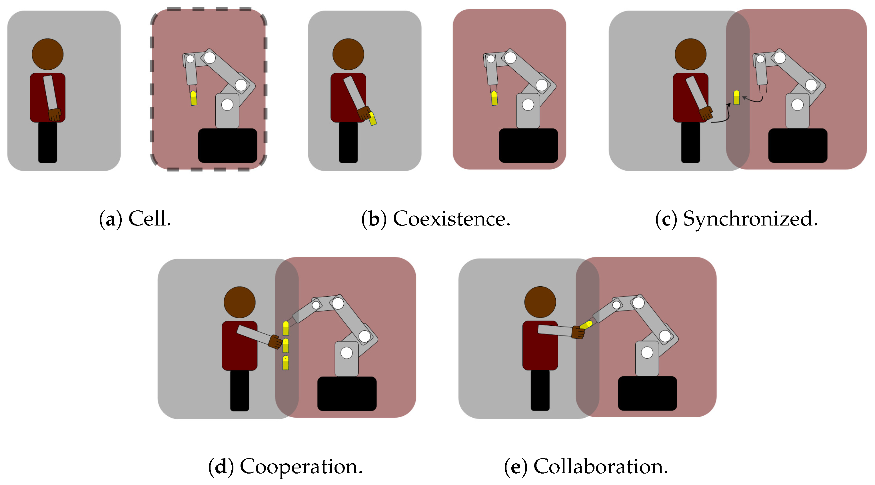
Figure 1. Human–robot cooperation levels in industrial environments. (a) The level cell involves no collaboration at all; the robot remains held inside a work cell. (b) Coexistence removes the cell, but humans and robots do not share the workspace yet. (c) Synchronized allows the sharing of the workspace, but never at the same time; humans and robots operate in a synchronized manner. (d) At the level cooperation, the task and the workspace are shared, but humans and robots do not physically interact. (e) The level collaboration considers full collaboration where operators and robots exchange forces.
Electronics 08 01306 g001
Figure 2. Proposed scenario inspired by an industrial collaborative robotic task in which the robot adapts its state to the human’s intention. (a) The force sensor is used to infer the human’s intention; the armband is used to inform the user about the robot’s internal state; and the piece adapter eases the grasping of the object. (b) While the robot holds the object, the human performs a frontal polishing of it.
Electronics 08 01306 g002
Figure 3. Mechanical dataset. Human movement patterns (left side) and appearance of the force signals produced by those patterns (right side). Observe how each class (ac) is quite distinguishable from the rest even after only 0.4 s. Making use of this dataset to train a model would allow predicting fast with enough confidence. Nevertheless, the movement patterns of the user would be too restricted, and the human–robot interaction would not be natural.
Electronics 08 01306 g003
Figure 4. Natural dataset. Human movement patterns (left side) and appearance of the force signals produced by those patterns (right side). Observe how each class (ac) is still similar to the rest even after 0.4 s. Due to the richness in movements, a model trained with this dataset would allow a natural human–robot interaction.
Electronics 08 01306 g004
Figure 5. Sampling windows evaluated to find an optimal classification-reaction time ratio. The windows correspond to: 0.1 s (cyan), 0.2 s (red), 0.5 s (green), 0.7 s (purple), and 1 s (orange). Recall that one second is our task limit time for achieving a suitable human–robot interaction.
Electronics 08 01306 g005
Figure 6. Dynamic Time Warping (DTW) for multi-dimensional time series: dependent (a) and independent (b) DTW. The former consists of computing the DTW similarity path of both dimensions (axis) at the same time. The latter is much simpler; normal DTW is computed separately on each dimension and their results added subsequently.
Electronics 08 01306 g006
Figure 7. F1-score values for the different types of raw data based classification (dependent and independent DTW), sampling window’s size (0.1, 0.2, 0.5, 0.7, and 1.0 s), and percentage of sub-sampling (where 100 means non-sub-sampling). The longer the sampling window, the better the classification performance. Observe how, for our task, a 0.5 s sampling window already provided a very good F1-score.
Electronics 08 01306 g007
Figure 8. Graphical representation of the values of the inference time per sample for the different types of raw data based classification (dependent and independent DTW), sampling window’s size (0.1, 0.2, 0.5, 0.7, and 1.0 s) and percentage of sub-sampling (where 100 means non-sub-sampling). The longer the window of data we consider, the longer the inference time. The total time to recognize the operator’s intent is the addition of the window’s size (horizontal axis) plus the inference time per sample (vertical axis).
Electronics 08 01306 g008
Figure 9. Global GPLVM inference process of the latent variables given a new sample in the higher dimensional space. First, the most similar training sample to the new sample is found using Euclidean distance. Second, the value of the latent variables of the most similar training sample (black dot in the first step) is used to initialize the inferred value (see the white dot in the second step). Third, the GPLVM model is optimized considering the new sample, which results in a refinement of the inferred latent variables. GPLVM with optimization includes the three steps; GPLVM without optimization stops after the second.
Electronics 08 01306 g009
Figure 10. F1-score values for the different types of feature based classification (optimized (op) and non-optimized GPLVM inference), sampling window’s size (0.1, 0.2, 0.5, 0.7, and 1.0 s), and number of latent variables (2, 3, 5, 10, and 20). Note that the bigger the number of latent variables, the better is the result, which also happens with the window size. Furthermore, observe that in some cases where the window’s size is very small (0.1 and 0.2 s), the shorter window outperforms the longer one by a small amount. This behavior is counter-intuitive, but possible due to the still negligible information contained within those small samples and the random selection of the training set.
Electronics 08 01306 g010
Figure 11. Graphical representation of the inference time per sample for the different types of feature based classification (optimized and non-optimized GPLVM inference), sampling window’s size (0.1, 0.2, 0.5, 0.7, and 1.0 s), and number of latent variables (2, 3, 5, 10, and 20). GPLVM-op leads to longer inference time than GPLVM, which also applies when the number of latent variables grows.
Electronics 08 01306 g011
Figure 12. Evaluation of the natural (blue) and the mechanical (red) datasets of the approach GPLVM + SVM without optimization and 10 latent variables. The mechanical data need less force information to classify with good quality. However, if the window of the force signal is large enough (more than 0.5 s), the model behaves similarly no matter whether the data are mechanical or natural.
Electronics 08 01306 g012
Figure 13. LED patterns used by the robot to communicate with the user using the robot’s armband. (a) Green pattern used to indicate when the robot is ready for physical interaction. (b) Red pattern indicating low classification confidence (<70%). Textual patterns showing the state of the robot when user intents are identified with high confidence: (c) “hold” (polish intent), (d) “move” (move intent), and (e) “open” (grab intent). The character “e” could not be expressed due to the four row armband matrix restriction.
Electronics 08 01306 g013
Figure 14. Normalized confusion matrix of the performance of the system during the validation with all users and trials. The matrix is non-symmetric, and the biggest portion of misclassified samples of the classes “grab” and “polish” are inferred as “move”, which indicates the existence of some bias in favor of the class “move”.
Electronics 08 01306 g014
Figure 15. Single perspective of the data visualization using the three most discriminating latent variables from the original ten. The distribution of the data in this lower space shows that the samples of the class “move” are rather close to the other two classes, which could be the reason why the model seems to be a bit biased in favor of this class.
Electronics 08 01306 g015
Figure 16. Average F1-score of the system for all the users along with the experiment’s trials. The positive slope of the trend line for the F1-score is an indicator of the adaptation of the users to the system. Please recall that none of the users followed the same sequential trial set since they were randomly generated.
Electronics 08 01306 g016