A Novel Nonlinearity Correction Algorithm for FMCW Radar Systems for Optimal Range Accuracy and Improved Multitarget Detection Capability

Abstract

Frequency-modulated continuous wave (FMCW) radars are an important class of radar systems, and they are quite popular because of their simpler architecture and lower cost. A fundamental problem in FMCW radars is the nonlinearity of the voltage-controlled oscillator (VCO), which results in a range of measurement errors, problems in multitarget detection, and degradation in synthetic aperture radar (SAR) images. In this paper, we first introduce a novel upsampling theory, then propose new algorithms to improve range accuracy and multitarget detection capability. These improvements are demonstrated both by simulations and actual lab experiments on a 2.4 GHz radar system. There are several techniques reported in the literature for VCO nonlinearity correction, but what makes the proposed approach different is that we focus on real-time processing on low-cost hardware and optimize the design subject to this constraint. We first developed an optimal upsampling theory which is based on almost-causal finite impulse response (FIR) filters. Compared to the sinc-based noncausal interpolation-based upsamplers, the proposed approach is based on using interpolation filters with few number of coefficients. Furthermore, interpolators are trained for a specific class of signals rather than a highly general signal set. Therefore, the proposed approach can be implemented on lower-cost hardware and perform quite well compared to more expensive systems.

1. Introduction

Compared to other types of radar systems, Frequency-modulated continuous wave (FMCW) radars can be built by simpler hardware and are commonly used in several different applications, including distance and velocity measurement, advanced driver assistance systems (ADAS), and synthetic aperture radar (SAR) imaging [1]. The key component in an FMCW radar is the voltage-controlled oscillator (VCO). The VCO output frequency is usually a nonlinear function of the input voltage, and this results in measurement errors and difficulty in separating targets. There are several known techniques to mitigate this problem. We first review some of the published research papers and discuss advantages/disadvantages of the proposed techniques. Later, we provide a more top-level discussion of known techniques and try to illustrate the novelty of the proposed method using a comparative analysis.

In [2], a 23 GHz phase locked loop design for FMCW radars is presented, and the linearity of the chirp signals is discussed from a chip design perspective. In this work, actual measurements of phase noise and chirp frequency errors are presented. However, the problem is addressed at the chip level, with a thorough discussion of different circuit design techniques to improve chirp linearity and to reduce VCO nonlinearity.

In [3], an FMCW radar operating at 1.9–3.7 GHz is presented. This work has a couple of similarities to our approach. First of all, it is a calibration-based technique, and an experimental verification is done by using “mini-circuit” discrete components. Nonlinearity correction is achieved by appyling a nonlinear control input to the VCO—more precisely, a fifth order control signal is used to produce linear frequency sweeps. In [3], the main focus was SAR imaging rather than automotive radars specific problems.

In [4], a pure simulation-based study was reported for nonlinearity correction of automotive radars. This approach is based on modeling the phase signal by a polynomial model, specifically, a cubic model. Although simulations with multiple targets are presented, a case of two closely spaced targets, e.g., a pedestrian walking in front of a bigger vehicle, was not simulated. Indeed, in [4], the ratio of target distances is always taken as two or larger in all simulations. This method is based on estimating the VCO nonlinearity and target distances at the same time. If the chirp signal is sampled at a very high rate, and we do have abundant information/samples, the proposed method is expected to have better performance. It is a computationally demanding technique, and the success rate is limited by the accuracy of the assumed model, and it is likely to have performance problems for closely spaced targets. In [5], an empirical mode decomposition (EMD)-based approach is introduced. The EMD method, also known as the Hilbert–Huang transform, is a heuristic decomposition technique. When there are two closely spaced targets, for example, a pedestrian walking in front of a vehicle, it may not detect two separate targets. Furthermore, there is no theoretical proof for the performance of the EMD method. However, simulation results presented in [5] illustrate that without modeling and calibration, it may sometimes work quite well. However, the same paper also has simulation examples where the performance is not that good.

In [6], another pure simulation-based work was presented. In this work, a nonlinear phase error was assumed to be measured or estimated from raw-data. In other words, a calibration-like procedure was used without an explicit polynomial model for the phase error. Basically, a table-based approach was adopted for storing the phase error information. Furthermore, as in [4], closely spaced targets were not simulated. In [7], a Cepstrum-based technique, called the homomorphic deconvolution, was proposed. Extensive simulation results were presented to demonstrate the effectiveness of the proposed approach. This method also requires a calibration procedure using a delay line.

Another related result is [8]. In this work, the phase error was approximated by a higher-order polynomial, but then instead of the regular fast fourier transform (FFT), a matched Fourier transform (MFT) approach was adopted. The computational complexity of this MFT approach grows quadratically with the number of samples, and this is a major drawback of this method. In this simulation-based paper, bandwidth was assumed as 5 GHz, but this high value is not easy to achieve around the frequencies considered. However, the sampling frequency of the beat signal was selected as 44.1 kHz, which is similar to the sampling frequencies adopted in our work. In [9], another calibration-based method was proposed. Compared to other known techniques, both amplitude and phase corrections were considered. Indeed, we have also observed some small fluctuation in the beat signal amplitude; however, its effect on the spectral analysis was quite small. Therefore, our proposed approach does not try to compensate for the amplitude fluctuations of the beat signal.

Another related result is [10]. This is basically a frequency domain technique, called the residual video phase removal. This is also a calibration-based technique and models the VCO frequency as a quadratic expression. Pure simulation results were presented at 10 GHz. In [11], VCO was modeled by a cubic expression, and a polynomial fit-based approach was proposed for nonlinearity correction. Basically, polynomial fit is again a kind of calibration procedure using a target at a known distance.

In [12], a nonlinearity correction algorithm that is based on time warping and an optimization using a spectral concentration measure was developed. This is also a simulation-based work, and a cubic phase nonlinearity was assumed. As is clearly stated in that paper, the proposed method was based on a grid search-based optimization, which can get computationally demanding for a dense grid. Hence, for real-time applications, it may have serious implementation difficulties. In [13,14], a higher-order instantaneous momentum (HIM)-based technique was introduced. However, as in [12], there are certain computational issues. First of all, it is an iterative technique. Furthermore, HIM expressions have combinatorial exponents, which are computationally expensive to evaluate, and they all have low noise immunity.

In [15], a direct digital synthesis (DDS)-based system was used together with a quadratic nonlinearity model and time resampling. The DDS method is a very powerful technique for generating single tone (frequency) sinusoidal signals, and the fundamental frequency was generated with very high precision. However, there is always some background noise in the DDS output. Furthermore, to generate a chirp signal of bandwidth, B, using DDS, the clock speed of the digital DDS equipment should be a couple of times higher than B. More importantly than all of these, to generate a chirp at a couple of GHz or higher levels, we still need an analog mixer, which will have its own noise and distortion.

In [16], a quadratic VCO model was assumed, but these parameters were estimated from specific corner reflectors in the area. Although there is no precalibration, there were certain reference targets in the environment with known location information. This was first used to estimate current VCO parameters, then these estimated parameters were used for image reconstruction. Basically, the use of corner reflectors with a known location info is a kind of autocalibration procedure, and without these specific reflectors, the method will not work properly. In [17], empirical mode decomposition (EMD) was used for UAV classification. This is also a nonmodel-based technique without a precalibration requirement. However, as in most heuristic techniques, we do not have a performance guarantee, and there are no reported performance data for two closely spaced targets and/or UAVs. In [18], an FMCW radar was used for vital signs monitoring. In this work, a quite different adaptive approach based on linear mean square (LMS) filtering was proposed. To reduce side lobes and hence improve the multitarget detection capability of the system, a windowing-based approach was adopted. More specifically, the Hanning window was used to preprocess data before the spectral analysis. In [19], we see again a circuit theory-based approach to improve chirp nonlinearity. In this work, a 23 GHz band radar design was considered, and the phase noise of the chirp generator circuit was measured. A quite different approach based on estimator design techniques was proposed in [20]. In this work, both the chirp rate and the initial chirp frequency were estimated from measurement data which were assumed to be corrupted by additive white Gaussian noise. However, a more idealistic second order VCO model was adopted, and performance analysis was done using only simulations. Finally, the authors of [21] included a discussion of other techniques and hardware acceleration-related aspects of the problem.

Table 1. Some of the known nonlinearity correction techniques.

Method Classification	References
Circuit level techniques	[2,19]
VCO control signal manipulation	[3]
No-calibration based	[4,5,17]
Nonmodel-based calibration	[6,7]
Model-based calibration	[8,9,10,11,16,20]
Computationally difficult	[12,13,14,18,22]
Time resampling	[15]

summarizes some of the known nonlinearity correction techniques.

Basically, we did not address the nonlinearity correction problem at the chip or circuit level; instead, we adopted a signal processing-based approach. The paper [3] is different than all of the others in the sense that, instead of using digital signal processing techniques with a sawtooth input to the VCO, VCO itself is driven by a nonstandard signal source to linearize its output frequency. However, it does have a calibration procedure, as in most of the methods reported in the literature. There are two interesting papers [4,5,17], which do not require calibration. However, their performance for closely spaced targets is either not that good or not fully investigated. Furthermore, we do not have theoretical proof for their performance. Most of the other techniques have some kind of calibration using a polynomial model and/or a look-up table. A few of these techniques are computationally quite demanding, using either a grid search or an iterative process.

The method proposed in the paper also has a calibration procedure; however, it is closer to the time resampling approach of [15]. In [15], a quadratic VCO model was assumed for time resampling. However, we propose a nonmodel-based approach to time resampling. More precisely, we considered optimal interpolators for time resampling. Compared to all of these techniques known in the literature, our fundamental difference is that we focus on methods which are optimized for real-time processing on low-cost hardware. The main motivation for this research direction was to find a solution which is better-suited for mass production of radars in autonomous vehicles.

Time-resampling techniques require estimation of the beat signal at different time instants using uniformly sampled beat signal data. One possibility is to use linear interpolation (“Standard” interpolation), but this may not be always very accurate. The other option is to use sinc function-based noncausal interpolators (Nyquist reconstruction); however, this approach may require a large number of filter coefficients. Furthermore, this technique requires first storing all beat signal data in a RAM array and then doing noncausal interpolation on this RAM array. This noncausal processing approach causes major problems in real-time applications. What is proposed in this paper is basically an optimal upsampling theory, and interpolating filters which are optimized (or trained) for a specific class of functions. The training class is a much “smaller” set compared to the band-limited or band-pass signals. Compared to the sinc-based noncausal interpolators, the proposed approach is based on using interpolation filters with a small number of coefficients. Indeed, all of the interpolation filters used in this paper need a maximum of two samples before and after the current sample, called the (–2,2) configuration. Because of this, the proposed algorithm can be implemented easily on a real-time system with limited buffering. Indeed, using any extra information available for the signals to be interpolated results in more accurate interpolators. The effectiveness of this approach is illustrated first on a simple case, and then later on FMCW radar systems using both simulations, and experimental data.

Time-resampling techniques require estimation of the beat signal at different time instants using uniformly sampled beat signal data. One possibility is to use linear interpolation (“Standard” interpolation), but this may not be always very accurate. The other option is to use sinc function-based noncausal interpolators (Nyquist reconstruction); however, this approach may require a large number of filter coefficients. Furthermore, this technique requires first storing all beat signal data in a RAM array and then doing noncausal interpolation on this RAM array. This noncausal processing approach causes major problems in real-time applications. What is proposed in this paper is basically an optimal upsampling theory, and interpolating filters which are optimized (or trained) for a specific class of functions. The training class is a much “smaller” set compared to the band-limited or band-pass signals. Compared to the sinc-based noncausal interpolators, the proposed approach is based on using interpolation filters with a small number of coefficients. Indeed, all of the interpolation filters used in this paper need a maximum of two samples before and after the current sample, called the (–2,2) configuration. Because of this, the proposed algorithm can be implemented easily on a real-time system with limited buffering. Indeed, using any extra information available for the signals to be interpolated results in more accurate interpolators. The effectiveness of this approach is illustrated first on a simple case, and then later on FMCW radar systems using both simulations, and experimental data.

Throught the paper, we use a couple of new concepts which are defined as follows: A linear shift invariant system with impulse response $h[·]$ is a compactly supported filter (CSF) if $\exists N_1,N_2\in \mathbb{Z}$ such that $h\left[k\right]=0$ if $k\notin [N_1,N_2]\cap \mathbb{Z}$. Note that this definition allows the filter h to be noncausal. A filter $h[·]$ which is equal to zero at all negative integers expect for finitely many points is called almost-causal. A CSF filter is both almost-causal and has finite impulse response. For true real-time implementation, causality is a must. However, if the application can tolerate a couple of sampling times delay compared to a true real-time implementation, CSF filters can be used for real-time processing, too.

This paper is organized as follows: In Section 2, we provide some background information about FMCW radars and present some preliminary experimental data on VCO nonlinearity to better illustrate the problem. In Section 3, we propose a new approach to upsampling theory. In Section 4, we explain the core idea proposed in this paper, which is the use of optimal upsampling interpolators for time resampling. In Section 5 and Section 6, we demonstrate the effectiveness of the proposed approach using both simulations and experimental measurements. In summary, we are able to get performance levels very close to “hardware resampling” without using additional hardware. Finally, in Section 7, we make some concluding remarks.

2. FMCW Radars and Preliminary Experimental Data on VCO Nonlinearity

A simplified block diagram of an FMCW radar system with a single antenna and directional coupler is shown in Figure 1. It is possible to have separate transmit and receive antennas without the directonal coupler, and more advanced systems may have multiple transmit and receive antennas to determine the target direction. The oscillator in the figure is a voltage-controlled oscillator (VCO) with output frequency depending on the input voltage, and this dependence is usually a nonlinear one. If the VCO has perfectly linear output frequency versus input voltage characteristics and $V_{\mathrm{tune}}$ is a sawtooth signal, the beat signal $s_b(t)$ will have “frequency” proportional to the target distance.

In this subsection, we provide some experimental data about the 2.4GHz VCO with part number ZX95-2536C+ (available from Mini-Circuits) and study the level of nonlinearity and its effects on range estimation. If the FMCW radar transmit signal is $s_t(t)=A(t)sin(2\pi {\int }_0^t{f}_T(q)dq)$ and we have a target at distance R, then beat signal will be $s_b(t)\approx A_b(t)sin(2\pi f_T(t)\tau +{\theta }_b)$ where $\tau =2R/c$, and c is the speed of light. Both $A(t)$ and $A_b(t)$ are low-frequency signals. In FMCW radars, the beat signal can be measured, and its frequency can be estimated using measured data. Furthermore, using the frequency estimate, one can easily predict the target distance R. However, if the VCO has a nonlinear characteristic, $f_T(t)$ will be a nonlinear function, and the beat signal will not be a pure sinusoid. In other words, the beat signal will have multiple frequency components, and the frequency estimation problem will be “ambiguous”. Furthermore, the spectrum of the beat signal will be spread over a wider frequency range with multiple larger side lobes, which will result in difficulties in multitarget detection. In the following table, we have the input voltage and measured output frequency values for the 2.4 GHz VCO ZX95-2536C+.

Table 2. Input voltage and measured output frequency table for the 2.4 GHz VCO ZX95-2536C+.

Input Voltage (V), ${\mathit{v}}_{\mathit{in}}$	Measured Output Frequency (MHz), ${\mathit{f}}_{\mathit{T}}(\mathit{t})$
0.00	2240
1.00	2314
2.00	2385
3.00	2456
4.00	2523
5.00	2577

was not extracted from the manufacturer’s datasheet; it was obtained by using a Keysight CXA Signal Analyzer N9000A with maximum input frequency of 3 GHz.

It is clear that this table represents a nonlinear behavior. In Figure 2, we show a measured beat signal for this particular VCO. To get the best possible experimental data for the single target case, we used a coaxial cable-based delay line which guarantees single reflection. Theoretically, the beat signal must be a single tone sinusoidal signal; however, the measured beat signal’s instantaneous frequency and amplitude are time-varying, and both quantities decrease from the beginning of the chirp to the end, as seen in Figure 2.

Because of the ambiguity in the frequency of this beat signal, we will have errors in the range estimation. Furthermore, the spectrum of such beat signals has larger side lobes, which will cause difficulties in multitarget detection. For a more detailed analysis of the measured data, see Section 6.

For a nonlinear VCO, the phase of the beat signal will not be a linear function of time. There is a linearization technique called time resampling discussed in Section 4, which is based on sampling the beat signal at a nonuniform rate so that the phase will be a linear function of the sample index. However, true nonuniform sampling requires complicated hardware and is usually avoided. Instead, the same effect is emulated either by sampling the beat signal uniformly at a much higher rate, which requires more expensive hardware, or using interpolation filters on uniformly sampled data measured at moderate sampling rates. Depending on how these interpolation filters are designed, we can get varying results.

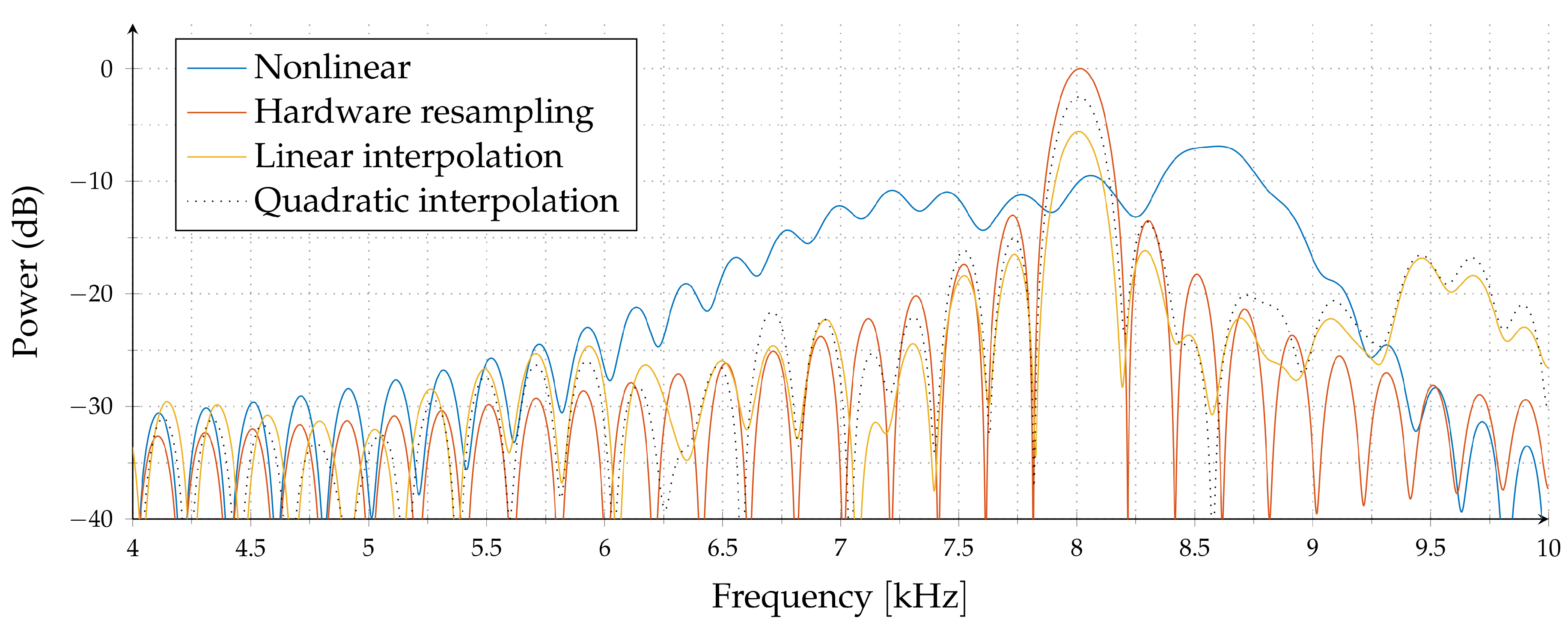
In Figure 3, we have a nonlinear VCO simulation for $f_T(t)=f_0+(t/T_{\mathrm{m}})f_{\mathrm{sweep}}-0.1{(t/T_{\mathrm{m}})}^3{f}_{\mathrm{sweep}}$, where $f_0=2.2\mathrm{GHz}$, $f_{\mathrm{sweep}}=0.4\mathrm{GHz}$ and $T_{\mathrm{m}}=5\mathrm{ms}$ is the chirp duration. The blue line is the spectrum of the beat signal without any correction. Note that the peak location and, hence, the range estimate has about 10% error. The red line is the spectrum for true hardware resampling, i.e., sampling the beat signal nonuniformly. The orange and dotted lines correspond to the spectrum of linear and quadratic interpolation of a uniformly sampled beat signal for a moderate sampling rate of $20\mathrm{kHz}$. Compared to true nonuniform sampling, we observed weaker main lobes, and more side lobes in linear and quadratic interpolators.

In Section 6, we demonstrate that the algorithms proposed in this paper have performance levels very close to true hardware resampling. Indeed, the spectrum obtained using the proposed optimal interpolation filters is almost the same as the spectrum obtained by at least 50 times higher sampling rate with linear interpolation. This is basically the most significant contribution of this paper.

In the following section, we focus on the optimal interpolation filter design problem.

3. A New Approach to Upsampling Theory

In this section, we introduce a new upsampling theory, which we call optimal upsampling. The standard upsampling theory is based on the theory of perfect reconstruction of band-limited or band-pass signals [24]. To upsample by a factor of $L\in {\mathbb{Z}}^{+}$, the first step is the expansion procedure, where $(L-1)$ zeros are added after each sample. The next step is called interpolation, where the ideal low-pass filter with a cut-off angular frequency of $\pi /L$ is used. Because of this filter being noncausal, and not compactly supported, truncation is necessary. However, it is known that the sinc function dies rather slowly, and several terms may be necessary for an accurate upsampling operation. Furthermore, noncausality is not desirable for real-time implementation.

The proposed upsampling theory differs from sinc-based upsampling theory in multiple different aspects. First of all, we considered a specific class of continuous time signals $\mathcal{S}$ rather than just band-limited or band-pass signals. For example, our specific signal class can be equal to finite-duration chirp signals with partially known parameters, and we may be interested in optimal upsampling only in a finite interval for this specific class of functions. The second difference is that we imposed the almost-causality as a constraint and minimized the reconstruction error subject to a fixed filter structure. Therefore, the resulting upsampler will use all of the information available about the continuous time signal and will be optimally subject to a realistic filter structure. Here, realistic means “of reasonable complexity from a real-time implementation perspective”.

Let us assume that we have a known class of continuous time signals $\mathcal{S}$, and an unknown continuous time signal $x(t)\in \mathcal{S}$ which is sampled at frequency $f_{\mathrm{s}}$ or period $T_{\mathrm{s}}$. We also assume that $x\left[n\right]=x(n{T}_{\mathrm{s}})$ values are known for some or all $n\in \mathbb{Z}$. To upsample by a factor of L, we first solve the least squares problem:

$$\underset{c}{min}\underset{f\in \mathcal{S}}{\mathbb{E}}|f((n+r/L)T_{\mathrm{s}})-\sum _{k=-p_1}^{p_2}{c}_{n,r,k}f((n+k)T_{\mathrm{s}}){|}^2,$$

(1)

for each $r\in [0,L-1]\cap \mathbb{Z}$, where ${\mathbb{E}}_{f\in \mathcal{S}}$ represents averaging over the set $\mathcal{S}$. If analytical solution is difficult, averaging can be done by selecting a large number of random signals in $\mathcal{S}$. This is called the $(-p_1,p_2)$ configuration, which means the interpolator needs $p_1$ samples before and $p_2$ samples after the current sample.

In this framework, the final upsampling equation will be:

$$x(m(T_{\mathrm{s}}/L))\approx \sum _{q\in \mathbb{Z}}{x}_{\uparrow L}\left[q\right]h[m,q],$$

(2)

where $x_{\uparrow L}[·]$ is the expanded signal, and $h[m,q]=c_{⎣m/L⎦,m\mathrm{mod}L,⎣q/L⎦-⎣m/L⎦}$. In general, $h[m,q]$ represents a time-varying filter for interpolation. However, if the coefficients $c_{n,r,k}$ do not depend on n, then there exists a function $g[·]$ such that $h[m,q]=g[m-q]$ for $L\mid q$. In this case, Equation (2) will reduce to the time-invariant interpolator, $x(m(T_{\mathrm{s}}/L))\approx {\sum }_{q\in \mathbb{Z}}{x}_{\uparrow L}\left[q\right]g[m-q]$.

For time-invariant filter design, instead of the pointwise minimization of the error as in Equation (1), one may consider the minimization of the sum of squares of errors and formulate an alternative objective function as:

$$\underset{c}{min}\underset{n}{\mathbb{E}}\underset{f\in \mathcal{S}}{\mathbb{E}}|f((n+r/L)T_{\mathrm{s}})-\sum _{k=-p_1}^{p_2}{c}_{n,r,k}f((n+k)T_{\mathrm{s}}){|}^2,$$

(3)

where ${\mathbb{E}}_n$ is averaging over the acquired samples.

To illustrate this procedure, let us consider pure sinusoidal signals of unknown frequency between 2400 and 2500 Hz and select the upsampling factor as $L=4$. Note that what we assume to know about the continuous time signal is more than the signal being band-limited from 2400 to 2500 Hz. Basically, we have an application where continuous time signals are known to be a pure sinusoidal signals of frequency from 2400 up to 2500 Hz, we have samples of the continuous time signal for $f_{\mathrm{s}}=6300\mathrm{Hz}$, and we would like to upsample by a factor of 4. Using a simple MATLAB script, we can find the solution of the least squares problem as:

$$\begin{array}{ccc}\hfill x(0T_{\mathrm{s}}/4)& \approx & +0.00x(-T_{\mathrm{s}})+1.00x(0T_{\mathrm{s}})+0.00x(T_{\mathrm{s}})\hfill \\ \hfill x(1T_{\mathrm{s}}/4)& \approx & -0.36x(-T_{\mathrm{s}})+1.00x(0T_{\mathrm{s}})+0.60x(T_{\mathrm{s}})\hfill \\ \hfill x(2T_{\mathrm{s}}/4)& \approx & -0.39x(-T_{\mathrm{s}})+0.95x(0T_{\mathrm{s}})+1.18x(T_{\mathrm{s}})\hfill \\ \hfill x(3T_{\mathrm{s}}/4)& \approx & -0.19x(-T_{\mathrm{s}})+0.65x(0T_{\mathrm{s}})+1.38x(T_{\mathrm{s}})\hfill \end{array}$$

and hence obtain $g[·]=(0.60,1.18,1.38,\underline{1},1,0.95,0.65,0,-0.36,0.39,$ $-0.19)$ where the underlined number represents the origin. This will be an upsampling system specifically optimized for sinusoidal signals of frequency from 2400 up to 2500 Hz. This interpolator can be realized on a real-time system with a delay of three $T_{\mathrm{s}}$ only.

4. Time Resampling Using Optimal Upsampling

In this section, we first introduce the standard time resampling approach and then illustrate what kind of improvements can be made using optimal upsampling. The FMCW radar setup that we consider has a voltage controlled oscillator (VCO) with transmit frequency $f_{\mathrm{T}}(t)$, which may or may not be a linear function of time. The transmitted signal is given by:

$$s_{\mathrm{T}}\left(t\right)=sin\left(\underset{\varphi \left(t\right)}{\underbrace{2\pi {\int }_0^t{f}_{\mathrm{T}}\left(q\right)\mathrm{d}q}}\right),$$

and if there is a single target, the received signal will be $s_{\mathrm{R}}(t)=s_{\mathrm{T}}(t-\tau )$ where $\tau =2R/c$, and R is the target distance. For moving targets, R will be a function of time. These two signals, $s_{\mathrm{T}}(t),s_{\mathrm{R}}(t)$ are multiplied and the result is low-pass filtered. This gives us what is called the beat signal, $s_{\mathrm{b}}(t)=\mathrm{LPF}\left\{2s_{\mathrm{T}}(t)s_{\mathrm{R}}(t)\right\}$ where LPF represents the low-pass filtering operation. Note that:

$$s_{\mathrm{b}}(t)=sin(\varphi (t)-\varphi (t-\tau )+{\theta }_{bb})=sin\left({\int }_{t-\tau }^t{f}_{\mathrm{T}}(q)\mathrm{d}q+{\theta }_{bb}\right)\approx sin(2\pi f_{\mathrm{T}}(t)\tau +{\theta }_{bb}).$$

If $f_{\mathrm{T}}(t)$ is not a linear function of time, the beat signal will not be a pure sinusiodal signal and the FFT spectrum of the sampled beat signal will have wider peaks and bigger side lobes. This is known to result difficulty in multiple target detection. For linear VCOs, the beat frequency and the target distance are related to each other by a very simple formula. However, for nonlinear VCOs, this is no longer the case.

For a nonlinear VCO, the phase of the beat signal, ${\varphi }_{\mathrm{b}}(t)=2\pi f_{\mathrm{T}}(t)\tau +{\theta }_{bb}$, will be assumed to be monotonic in time. Sampling at regular time intervals will result in nonconstant increments in phase. The time resampling approach is based on sampling, $s_{\mathrm{b}}(t)$, at nonuniformly spaced time instants such that the resulting phase increments are constant. To find these resampling instants, we need to solve:

$$f_{\mathrm{T}}(t_k)-f_{\mathrm{T}}(t_0)=k\left(\frac{f_{\mathrm{T}}((N-1)T_{\mathrm{s}})-f_{\mathrm{T}}(0T_{\mathrm{s}})}{(N-1)T_{\mathrm{s}}}\right),k=1,\cdots ,N-1.$$

Sampling at these new $t_k$’s will result a different sampled signal which has a constant frequency in the discrete time domain, which in turn can be estimated using the standard FFT-based techniques. Determination of resampling instants is a kind of precalibration procedure which can be done using a delay line.

Now consider a precalibrated FMCW radar system. Sampling $s_{\mathrm{b}}(t)$ at irregular time intervals will require additional nonstandard hardware. A commonly used alternative approach is approximating $s_{\mathrm{b}}(t_k)$ values from regularly sampled values, $s_{\mathrm{b}}(k{T}_{\mathrm{s}}),k=0,\cdots ,N-1$. If the sampling frequency $f_{\mathrm{s}}$ is sufficiently high compared to the frequency of $s_{\mathrm{b}}(t)$, then linear interpolation can be used to estimate $s_{\mathrm{b}}(t_k)$ values. However, if the target is not very close, i.e., the beat frequency is not quite small compared to the sampling frequency, linear interpolation will result in larger errors, and accurate estimation $s_{\mathrm{b}}(t_k)$ values will have crucial importance.

The main contribution of this paper can be summarized as follows: Instead of using a standard linear interpolation approach to estimate $s_{\mathrm{b}}(t_k)$ values, we used an optimal upsampler designed for the class of signals in which we are interested. We illustrated the advantages of this optimal upsampling approach using both simulations and experimental verification.

5. Simulation Results

We have a 2.4 GHz radar setup using the minicircuits VCO with part number ZX95-2536C+. We used a Keysight N9000A spectrum analyzer to measure VCO output frequency and amplitude, and using measured data, we generated a table for the simulation of this particular VCO. Python based scripts were used to simulate a target at 15 m with a sweep duration of 10 ms. The beat signal is denoted by $s_{\mathrm{b}}(t)$. Then both standard interpolation and optimal upsampling-based interpolation were used to estimate $s_{\mathrm{b}}(t_k)$ values from regularly sampled data. The optimal upsampler was optimized for the class of beat signals corresponding to target distance $d_{\mathrm{o}}\pm 15\%$, where $d_{\mathrm{o}}$ is the distance estimate obtained by the standard linear interpolation-based approach.

The result of this simulation study is presented in Figure 4. It is clear that if we use the information available about the VCO and set of possible beat signals that we can observe in such an experiment (with $\pm 15\%$ error included) and then use an optimized interpolator for upsampling, we do observe improvements in the spectrum. In particular, after optimal upsampling, side lobes are reduced, which will result in an improved multitarget detection performance. Furthermore, peaks are a couple of dBs sharper too.

6. Experimental Verification

In this section, we demonstate the effectiveness of the proposed approach using actual experimental data.

Table 3. Lab equipments and RF components used in experiments.

Equipment	Details
Voltage controlled oscillator (VCO)	Mini-circuits VCO ZX95-2536C+ (2.4 GHz)
Low-noise amplifier (LNA)	Mini-Circuits ZX60-272LN-S+
Splitter	Mini-Circuits ZX10-2-42+
Mixer	Mini-circuits 1ZX05-43MH-S+
Low-pass filter	15 kHz active 4th-order
Signal Analyzer	Keysight CXA Signal Analyzer N9000A (3 GHz)
Mixed Signal Scope	Tektronix MDO 3104 (5 GS/s sample rate)
Signal Generator	Tektronix AFG3052C

summarizes lab equipments and RF components used in experiments.

To verify the effectiveness of the proposed approach, we did an experiment with the same VCO together with an LNA, splitter, and mixer (See Figure 5). We used a delay line to make sure that experimental measurements are repeatable. We recorded the beat signal at 441 kHz, which is quite high and used only for comparison purposes. The result of the time resampling for this 441 kHz sampling frequency is shown in Figure 6. We also recorded the same beat signal at 6300 Hz, and used this for standard interpolation-based time resampling. Finally, these 6300 Hz data were optimally upsampled to estimate $s_{\mathrm{b}}(t_k)$ values from regularly sampled data. The resulting spectrums are shown in Figure 6. It is clear that optimal upsampling results in a better spectrum with a sharper main lobe and weaker side lobes. Furthermore, spectrums for optimally upsampled data and true hardware resampled data are very close to each other.

To do the optimal upsampling, we did not use any information available in the datasheet of the VCO. Instead, we simply used a upsampler trained for sinusoidal signals of frequency from 2500 to 2700 Hz. Basically, training the interpolator for a more specific class of functions rather than more general band-pass or band-limited functions results in an improved performance.

7. Conclusions

In this paper, we studied the design of FMCW radars on low-cost hardware and what kind of signal processing techniques can be developed for improved performance. A fundamental constraint that we imposed was ease of real-time implementation on low-cost hardware, in particular, almost-causality of interpolation filters. We have introduced a new upsampling theory based on fixed structure interpolators optimized/trained for a specific class of functions. This results in very effective interpolators having CSF property. Application of this theory for FMCW radar nonlinearity correction resulted in improvements in the spectrum, specifically for suppressing the side lobes and sharpening the main lobe. This is known to improve multitarget detection performance.