Online Slack-Stealing Scheduling with Modified laEDF in Real-Time Systems

Abstract

In hard real-time task systems where periodic and aperiodic tasks coexist, the object of task scheduling is to reduce the response time of the aperiodic tasks while meeting the deadline of periodic tasks. Total bandwidth server (TBS) and advanced TBS (ATBS) are used in dynamic priority systems. However, these methods are not optimal solutions because they use the worst-case execution time (WCET) or the estimation value of the actual execution time of the aperiodic tasks. This paper presents an online slack-stealing algorithm called SSML that can make significant response time reducing by modification of look-ahead earliest deadline first (laEDF) algorithm as the slack computation method. While the conventional slack-stealing method has a disadvantage that the slack amount of each frame must be calculated in advance, SSML calculates the slack when aperiodic tasks arrive. Our simulation results show that SSML outperforms the existing TBS based algorithms when the periodic task utilization is higher than 60%. Compared to ATBS with virtual release advancing (VRA), the proposed algorithm can reduce the response time up to about 75%. The performance advantage becomes much larger as the utilization increases. Moreover, it shows a small performance variation of response time for various task environments.

1. Introduction

Modern complex real-time control systems should perform computationally intensive activities within a specified time duration. For example, to ensure both the correct reconfiguration of external signals and the stable operation of the system, the acquisition of sensor signals and the system control must be performed periodically until their time limit. Besides, to achieve predictable timing behavior and meet stability requirements, some control tasks may be characterized by stringent timing constraints that must be met on all anticipated workloads. On the other hand, some tasks, such as user interface tasks, do not require periodic execution but are triggered aperiodically when certain conditions occur. Also, they just need to respond as soon as possible.

A task whose deadline is determined by which the task should be satisfied in all task scenarios is called a hard task. Failure to meet the deadline for this task usually causes or contributes to catastrophic consequences. A soft task is defined that the deadline of a task is not restricted to its time limit. The task does not cause serious damage even if the deadline is missed. In the above-mentioned systems, the tasks related to both the acquisition of sensor signals and the system control are assigned to the hard tasks (i.e., hard real-time tasks). However, the tasks for the interfacing with users are assigned to the soft tasks (i.e., soft real-time tasks). The main scheduling objective with a mixed real-time control system (i.e., the system with the hard and soft tasks) is to provide excellent responsiveness to soft aperiodic tasks, ensuring that all hard tasks are executed within their time constraints. It means that the system must schedule aperiodic tasks as soon as possible, guaranteeing the time limit of periodic tasks.

The most simplified technique for handling aperiodic tasks is to allocate available time slots that are left unused by periodic tasks. Although this background scheduling is straightforward, the sufficient responsiveness is never acquired [1]. To reduce the response time of aperiodic tasks, the server concept was introduced and divided into the fixed and dynamic priority server according to servers priority changeability. The fixed priority servers in [2,3,4] are based on the rate monotonic (RM) algorithm [5], where the higher priority tasks have lower jitters. Although RM is an optimal solution, it is not generally possible to use 100% of the processor [5]. On the other hand, dynamic scheduling algorithms, such as the earliest deadline first (EDF), can be used to increase processor utilization [5]. Dynamic priority servers such as total bandwidth server (TBS) [2] and constant bandwidth server (CBS) [6] greatly affect the responsiveness of the aperiodic tasks.

The TBS algorithm was proposed in [2], where the deadline for an aperiodic task was scheduled under EDF. In the TBS algorithm, setting deadlines for aperiodic tasks is simpler than the traditional approaches. However, it has a limit on the deadline setting, since the algorithm uses the worst-case execution time (WCET) of each aperiodic task to set the deadline. Although tasks generally complete earlier than the WCET, the deadline is set by using the WCET in TBS. Therefore, the response time of the aperiodic task becomes worse. The advanced TBS (ATBS) was proposed in [7,8] to reduce the aperiodic task response time, where the deadline of the currently arrived aperiodic task is predicted based on the execution time of the previously performed aperiodic tasks. It was shown in [7] that the execution time of an aperiodic task is predicted by using the weighted average filter method. However, it was shown in [8] that the execution time of an aperiodic task is set by using the average filter method. The virtual release advancing (VRA) method was proposed in [9] to further reduce the response time of ATBS. The deadline for each aperiodic task in [9] is recalculated as soon as possible without affecting previously scheduled tasks.

The slack is the amount of time left after a job. Slack-stealing algorithm creates a slack stealer, which attempts to make time for servicing aperiodic tasks by stealing the processing time from the periodic tasks without causing their deadlines to be missed. Several slack-stealing methods have been proposed in [10,11,12]. However, they are all fixed-priority scheduling algorithms and offline methods. The laEDF [13] is a kind of dynamic scheduling. For power savings in a system, it is noted that the dynamic voltage scaling (DVS) method is used by lowering the frequency of processor within a possible range satisfying the deadline of periodic tasks. The laEDF algorithm calculates the frequency of a processor to satisfy the deadlines of future periodic tasks. In this paper, we propose an online slack-stealing method by using the modification of laEDF to improve the scheduling performance of mixed tasks in real-time systems. Unlike the existing slack-stealing method, the proposed algorithm operates under dynamic priority scheduling to increase processor utilization. Our simulation results show that slack-stealing with modified laEDF (SSML) outperforms the existing TBS based algorithms when the periodic task utilization is higher than 60%. Compared to ATBS with virtual release advancing (VRA), the proposed algorithm can reduce the response time up to about 75%. The performance advantage becomes much larger as the utilization increases.

2. System Design

We consider a preemptive real-time scheduling system with a uniprocessor on which tasks are scheduled under the EDF scheduling policy. The system consists of two types of tasks (i.e., the hard real-time periodic tasks and soft real-time aperiodic tasks). We assume that there is a input task set $\Psi$ consists of n periodic tasks (i.e., $T_1,T_2,\cdots ,T_n$) and aperiodic requests in the system. The i-th periodic task is defined by $T_i(C_i,P_i)$, where $C_i$ is the WCET and $P_i$ is its period. The processor utilization of $T_i$ is denoted by $U_i=C_i/P_i$. The total processor utilization of the periodic tasks in the system ($U_p$) can be represented as

$$U_p=\sum _{i=1}^n{U}_i=\sum _{i=1}^n\frac{P_i}{C_i}.$$

(1)

It is supposed that periodic tasks are released periodically once every $P_i$ time unit and its relative deadline $d_i$ is the same as its period $P_i$. We assume that all periodic tasks are ready at $t=0$. The aperiodic task is defined as $J_k$ with a 2-tuple ($r_{J_k}$, $C_{J_k}$), where $r_{J_k}$ and $C_{J_k}$ are the arrival time and WCET of $J_k$, respectively. Aperiodic tasks arrive sequentially and have uncertain deadlines, which means that the computational and arrival times are unknown in advance, respectively. It is also supposed that periodic and aperiodic tasks are independent and the context switching overheads and transition times are negligible.

We state our notation as follows :

$C_i$

denotes the WCET of a periodic task $T_i$. (i.e., the WCET needed by the processor to execute an instance of the task without interruption)

$C_{J_i}$

denotes the WCET of an aperiodic task job $J_i$.

$c\_lef{t}_i$

denotes the remaining computation time of the current instance of task $T_i$.

$d_i$

denotes the absolute deadline assigned to a periodic task $T_i$.

$d_{J_i}$

denotes the absolute deadline assigned to an aperiodic task job $J_i$ by the algorithm.

$r_i$

denotes the arrival time of a periodic task $T_i$.

$r_{J_i}$

denotes the arrival time of an aperiodic task job $J_i$. (i.e., the time at which the job is activated and becomes ready to execute)

$\sigma$

denotes slack until the earliest periodic task deadline.

$W_i$

denotes the response time of the i-th aperiodic task job.

3. The Slack-Stealing with Modified laEDF Algorithm

3.1. Look-Ahead EDF

The laEDF algorithm is shown in Algorithm 1. The major step in this algorithm is the defer() function. The function looks at the interval until the next task deadline, trying to push as much work as it can beyond the deadline. Then, it computes the minimum amount of work during this interval to meet all future deadlines. In Algorithm 1, the periodic tasks are sorted in reverse EDF order to calculate the minimum amount of work to be done until the next deadline in the defer() function. It checks whether $T_i$ can be executed between the earliest deadline($d_n$) and the deadline of the task($d_i$). If x is less than or equal to 0, it means that the task can be performed within this interval. In Algorithm 1, the utilization rate excluding the utilization of the periodic task $T_i$ is calculated by

$$U=U-C_i/P_i.$$

(2)

The amount of work for task $T_i$ until the earliest deadline is defined as

$$x=max(0,c\_lef{t}_i-(1-U)(d_i-d_n)),$$

(3)

where $d_n$ is the earliest deadline and ($1-U$) is the utilization that can be allocated to the task $T_i$. Then, U is updated to reflect the actual utilization of the task for the time after $d_n$. This calculation is repeated for all tasks.

$$U=U+(c\_lef{t}_i-x)/(d_i-d_n).$$

(4)

Algorithm 1 Look-ahead EDF(laEDF) algorithms.

1: function select_frequency(x) 2:     use lowest freq. $f_i\in f_1,\cdots ,f_m|f_1<\cdots <f_m$ such that $x\le \frac{f_i}{f_m}$ 3: end function 4:   5: upon task_release($T_i$) 6:     set $c\_lef{t}_i=C_i$ 7:     defer() 8:   9: upon task_complete($T_i$) 10:     set $c\_lef{t}_i=0$ 11:     defer() 12:   13: during task_execution($T_i$) 14:     decrement $c\_lef{t}_i$ 15:   16: function defer( ) 17:     set $U=C_1/P_1+\cdots +C_n/P_n$ 18:     set $s=0$ 19:     for i=1 do n 20:         set $U=U-C_i/P_i$ 21:         set $x=max(0,c\_lef{t}_i-(1-U)(d_i-d_n))$ 22:         set $U=U+(c\_lef{t}_i-x)/(d_i-d_n)$ 23:         set $s=s+x$ 24:     end for 25:     select_frequency $(s/(d_n-\mathrm{current}\_\mathrm{time}))$ 26: end function

In Equation (4), the processor utilization between $d_n$ and $d_i$ is updated with the amount of work excluding the work to be performed until $d_n$. The operating frequency at t is computed as

$$freq.=\frac{s}{d_n-t},$$

(5)

where s means the sum of work to complete up to the earliest deadline $d_n$.

Figure 1 shows an example of the laEDF algorithm, where 3 periodic tasks exist. The deadlines of tasks are $d_1$, $d_2$, and $d_3$, respectively. The deadlines are assumed as $d_3>d_2>d_1$. In the system, the processor is assumed that three normalized and discrete frequencies are available (i.e., 0.5, 0.75, and 1.0). In the algorithm, the goal is to defer work beyond the earliest deadline ($d_1$) in the system so that the processor can operate at a low frequency. The algorithm allocates time in the schedule for the worst-case execution of each task, starting the task with the latest deadline, $T_3$ (i.e., reverse EDF order). The algorithm spreads out $T_3$’s work between the earliest deadline ($d_1$) and its deadline $d_3$ (x of $T_3\le$ 0), subject to reserving a constant capacity for the future invocation of the other tasks. The algorithm repeats this step for $T_2$, which can not entirely fit between $d_1$ and $d_2$ (x of $T_2$ > 0) after the allocation of $T_3$ and reserving capacity for the future invocations of $T_1$. The remaining work for $T_2$ and all of $T_1$ are allotted before $d_1$. Therefore, the required minimum frequency is 0.55 to meet all periodic tasks’ deadline. As a result, the frequency of 0.75 can be applied at $t=0$.

3.2. The SSML Algorithm

The SSML algorithm takes advantage of the fact that the laEDF algorithm defers as many periodic tasks as possible to lower the frequency of the processor beyond the earliest deadline, satisfying the periodic tasks’ deadline. In the proposed algorithm, we use the fact that the laEDF algorithm calculates the amount of work to be done up to the earliest deadline to satisfy the deadlines. The SSML algorithm calculates the allowable time to an aperiodic task from the current time, the deadline of the earliest periodic task, and the work amount of the periodic task’s work to be done until that point. The SSML algorithm is shown in Algorithm 2.

Algorithm 2 SSML algorithms.

1: upon task_release($\tau$) 2:     if $\tau \in T_i$        /* $\tau$ is a periodic task */ 3:         set $c\_lef{t}_i=C_i;$ 4:     if there is aperiodic task in ready queue 5:         defer(); 6:   7: upon task_complete($\tau$) 8:     if $\tau \in T_i$        /* $\tau$ is a periodic task */ 9:         set $c\_lef{t}_i=0;$ 10:     if there is aperiodic task in ready queue 11:         defer(); 12:   13: during task_execution($\tau$) 14:     if $\tau \in T_i$        /* $\tau$ is a periodic task */ 15:         decrement $c\_lef{t}_i$ 16:     if $\tau \in J_k$        /* $\tau$ is an aperiodic task */ 17:         decrement $\sigma$ 18:         if $\sigma <=0$ 19:             defer(); 20:   21: function defer( ) 22:     set $U_p=C_1/P_1+\cdots +C_n/P_n$        /* n is a periodic task number */ 23:     set $U=U_p$ 24:     set $s=0$ 25:     for $i=1$do$n,T_i\in \{T_1,\cdots ,T_n|d_1\ge \cdots \ge d_n$} 26:         set $U=U-C_i/P_i$ 27:         set $x=max(0,c\_lef{t}_i-(U_p-U)(d_i-d_n))$ 28:         set $U=U+(c\_lef{t}_i-x)/(d_i-d_n)$ 29:         set $s=s+x$ 30:     end for 31:     $\sigma =d_n-(t+s)$;        /* t is a current time */ 32:     set_deadline($\sigma$); 33: end function 34:   35: function set_deadline($\sigma$) 36:     if $\sigma \ge 0$ 37:         set $d_{J_k}$ as the highest priority 38:     else 39:         set $d_{J_k}$ as low priority 40: end function

In lines 1–5, task_release is called when a new task is released. In this function, the task’s $c\_lef{t}_i$ becomes the WCET of the task because the actual execution time of the task is unknown. Then, the defer() function is called to calculate the slack ($\sigma$) if there is an aperiodic task in the task ready queue. In lines 7–11, task_complete is called when a task is completed. $c\_lef{t}_i$ of the task becomes 0. Then, if there is an aperiodic task in the task ready queue, the defer() function is called to check the available time of the aperiodic task. $c\_lef{t}_i$ is decremented as the task executes from line 15. If the executing task is an aperiodic task, $\sigma$ is also decremented. If the slack is equal to or less than 0 (i.e., lines 18–19), it means there is no time to allocate to the aperiodic task. Therefore, the defer() function is called to lower the aperiodic task’s priority. The defer() function in line 21–33 computes the amount of periodic tasks’ work to meet the earliest deadline. In line 22, the defer() function calculates the total utilization of periodic tasks. Then, line 25–30 is performed by arranging the tasks in reverse EDF order. In line 26, the utilization is obtained by subtracting the utilization of the i-th periodic task. At line 27 computes the amount of periodic task’s work to be done until the earliest deadline. Compared to Algorithm 1, it can be confirmed that $U_p-U$ is applied instead of $1-U$ to allocate as many processors as possible to the aperiodic task satisfying the deadline of the periodic task among the second argument of max function. In line 28, we can see that the amount of work to be performed between $d_n$ to $d_i$ of the i-th task is updated based on the amounts of work excluded ($c\_lef{t}_i-x$). It can be seen that s (i.e., the amount of work) of periodic tasks to be performed up to $d_n$ is calculated by adding x. In line 31, we can see that the slack of an aperiodic task is calculated by

$$\sigma =d_n-(t+s).$$

(6)

Based on the slack, the set_deadline() function is called to adjust the deadline of the aperiodic task. In lines 35–40, the algorithm sets the aperiodic task’s deadline according to the slack. If $\sigma >0$, then the highest priority is assigned to the aperiodic task to reduce the aperiodic task’s response time. On the other hand, if $\sigma <=0$ is less than or equal to 0, it means that there is no spare time to allocate to an aperiodic task. The priority of the aperiodic task is set lower than that of the periodic task to meet the deadline of the periodic tasks.

3.3. Illustrative Example

In this section, an example of TBS and SSML is described. In Figure 2a,b show the scheduling results of the TBS and SSML, respectively. We assume that there are three periodic tasks (i.e., $T_1$, $T_2$, and $T_3$) and an aperiodic task $T_4$. The period of $T_1$ is $P_1=2$, and its execution time $C_1=1$. $T_2$ has the period $P_2=5$, and its execution time $C_2=1$. $T_3$ has the period $P_3=10$, and its execution time $C_3=2$. Therefore, the total CPU utilization by three periodic tasks is 0.9.

$$U_p=\frac{1}{2}+\frac{1}{5}+\frac{2}{10}=0.5+0.2+0.2=0.9.$$

(7)

The CPU utilization by the aperiodic server can be $U_s=1-U_p=0.1$. In TBS, the k-th aperiodic request arrives at $t=r_{J_k}$, and the deadline is defined as

$$d_{J_k}=max(r_{J_k},d_{J_{k-1}})+\frac{C_{J_k}}{U_s},$$

(8)

where $C_{J_k}$ is the WCET of the request, and $U_s$ is the server utilization. In the example, 2 aperiodic jobs arrive at time 1 and 10. Their actual execution times are 0.2 and 0.5, respectively. The request is then inserted into a task ready queue of the system and scheduled by EDF along with any periodic instances. It is noted that we can keep track of the bandwidth assigned to other requests by taking the maximum between $r_{J_k}$ and $d_{J_{k-1}}$. Figure 2a shows an example of the TBS scheduling result. The first aperiodic request arrives at $t=1$ and is assigned a deadline

$$d_{J_1}=r_{J_1}+\frac{C_{J_1}}{U_s}=1+\frac{1}{0.1}=11.$$

(9)

Since $d_{J_1}$ is not the earliest deadline until $t=10$, the aperiodic job can not get the processor. But at $t=9$, there are no periodic tasks in task ready queue of the system. Therefore, the aperiodic job ($J_1$) starts execution and finishes at $t=9.2$. The second aperiodic request arrives at $t=10$. By the definition of the TBS, $d_{J_2}$ is calculated as

$$d_{J_2}=max(r_{J_2},d_{J_1})+\frac{C_J}{U_s}=11+\frac{1}{0.1}=21.$$

(10)

Since $d_{J_2}$ is not the earliest deadline until $t=20$. The aperiodic job can not get the processor. But at $t=19$, there are no periodic tasks in the task ready queue of the system. Then, the aperiodic job ($J_2$) starts execution and finishes at $t=19.5$, because its actual execution time is 0.5. Consequently, the response times of the two aperiodic jobs become $W_{1,TBS}=9.2-1=8.2$ and $W_{2,TBS}=19.5-10=9.5$, respectively.

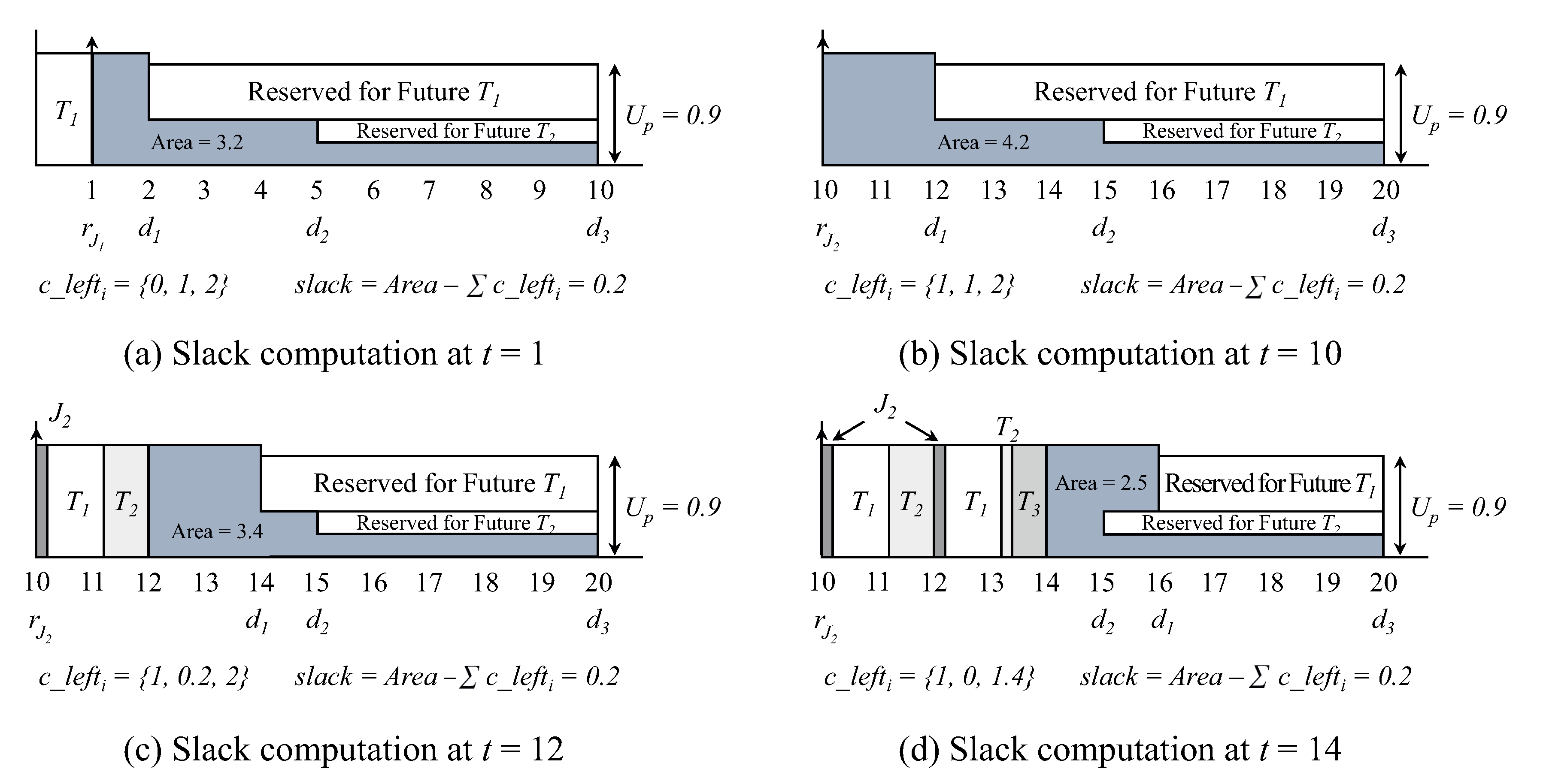
On the other hand, we can see that the response times of the aperiodic jobs are drastically reduced through Figure 2b. When the first aperiodic job arrives at $t=1$. The slack is calculated by the SSML algorithm. Figure 3a depicts the defer() function result. At $t=1$, $c\_lef{t}_1,c\_lef{t}_2,c\_lef{t}_3$ are 0, 1, and 2, respectively. As a result of the defer() function, the periodic task’s job should be done until the earliest periodic task’s deadline ($d_1=2$) is 0.8. By the line 28 in Algorithm 2, the slack is 0.2.

$$\sigma =D_n-(t+s)=2-(1+0.8)=0.2.$$

(11)

Since the slack is greater than zero, the aperiodic job must be assigned to the highest priority. Therefore, the aperiodic job can be performed first. Since the actual execution time of the first aperiodic job is 0.2, the task completes at $t=1.2$. Therefore, the first aperiodic task response time becomes $W_{1,SSML}=1.2-1.0=0.2$. The scheduling of subsequent periodic tasks is performed by the EDF algorithm. The second aperiodic job arrives at $t=10$. The result of the defer() function at the time is shown in Figure 3b. The $c\_lef{t}_i$ for 3 periodic tasks are 1, 1, and 2 respectively. The defer() function shows the workload of the periodic task to be performed until the $t=12$ (i.e., the earliest deadline) is 1.8, resulting in the slack being 0.2.

$$\sigma =12-(10+1.8)=0.2.$$

(12)

Therefore, the aperiodic task is performed for 0.2. Since the slack is exhausted at $t=10.2$, the periodic task $T_1$ is executed, because $T_1$ has the earliest deadline. Periodic tasks are performed until $t=12$. The result of defer() function at $t=12$ is shown in Figure 3c. The earliest deadline for periodic tasks is 14, and the amount of work for the periodic task to be performed up to this is found to be 1.8. Therefore, the aperiodic task is executing for 0.2 (i.e., $\sigma =14-(12+1.8)$), and the periodic task $T_1$ is executed again. The result of the defer() function at time 14 is shown in Figure 3d. In this case, the deadline for the earliest periodic task is 15, and the work to be performed until this time is 0.9. Therefore, the slack of 0.1 is used by the aperiodic job. Since the actual execution time of this aperiodic task is 0.5, the task completes its execution at $t=14.1$. Therefore, the response time of the second aperiodic job becomes $W_{2,SSML}=14.1-10=4.1$. Consequently, the response times of SSML are 0.2 and 4.1 respectively.

4. Evaluation

Here, we present the simulation results for evaluating the proposed algorithm, by comparing with TBS based schemes, which are the aperiodic task scheduling algorithms under the dynamic priority-driven systems. We compared the algorithms for the following six cases.

• SSML: slack-stealing method with modified laEDF as a slack computation method.
• Original TBS: a scheduling method for assigning the deadline for each aperiodic job by using its WCET
• ATBS: adaptive TBS with the deadline of each aperiodic job by using predicted execution time.
• ATBS+VRA: ATBS with VRA for improving the average response time of aperiodic tasks.
• ORACLE: a scheduling method for assigning the deadlines of aperiodic tasks, where OS can know the exact job amounts.
• ORACLE+VRA: ORACLE with VRA for improving the average response time of aperiodic tasks.

The performance of the algorithms was measured by computing the average aperiodic response time as a function of the periodic task utilization or the mean aperiodic load. In particular, each aperiodic response time has been normalized to its actual length. Thus, a value of 5 on the y-axis actually means an average response time five times longer than the actual task computation time. To understand how task parameters affect aperiodic task responsiveness, several simulations have been performed by changing the periodic load, average aperiodic computation time, and average aperiodic load.

The first simulation shows the performance of the algorithms to the periodic task loads for a given aperiodic load. The second simulation shows the performance results of the algorithm according to the change of the average execution time and the WCET of the aperiodic task. Finally, the third simulation illustrates the performance results with various aperiodic loads.

In all simulations, we selected 10 periodic task sets and 10 aperiodic task sets combining into 100 task sets. For periodic tasks, their periods are generated as a random variable, which is uniformly distributed from 50 to 200 ticks. The utilization of a periodic task was evaluated as a random variable, which is uniformly distributed from 0 to 1 and normalized to obtain the desired periodic utilization factor $U_p$. As for aperiodic task sets, we assume that an aperiodic task arrives multiple times where the arrival times are determined by Poisson distribution with 1.5 per 1000 ticks on average. We also assumed that the WCETs and actual execution times are decided by exponential distributions. The execution times were under the condition that the upper bound is the corresponding WCET. Each simulation has a duration of 100,000 ticks.

Figure 4 shows the average normalized response time (ANRT) ratio of the proposed algorithm as a function of periodic task utilization, comparing various algorithms. The total utilization of the periodic tasks varied from 60% to 90%. In the aperiodic tasks, the exponential distribution average of WCET (${\lambda }_{WCET}$) and actual execution time (${\lambda }_{AET}$) were eight and four ticks, respectively. In the simulations, the average ratio of the actual execution time with respect to WCET is 0.7, and the aperiodic task load was 0.03. The figure shows that, under 65%, the response times are almost the same for all the six cases. This is because the server utilization (i.e., $U_s=1-U_p$) is large enough to quickly serve the aperiodic requests. We also see that over 70%, the performance gain of the proposed algorithm can be increased. At $U_p=0.9$, the ANRT of the proposed algorithm is about 3.5, whereas that of the ATBS with VRA is about 13.47. Simulation results show that the algorithm can reduce response times by up to 75% compared with ATBS with VRA. In addition, it can be seen that the response time is about 2 times faster than the result of ORACLE with VRA. It means that the TBS based algorithm can conservatively set the deadline for each task job even if the actual execution time of each job is known. And it can be seen that the response time of the aperiodic task increases significantly when the utilization of the periodic task becomes more inefficient.

Figure 5 shows the ANRT of the proposed algorithm as a function of periodic task utilization when the average value of the WCET(${\lambda }_{WCET}$) and actual execution time (${\lambda }_{AET}$) are 80 and 40 ticks with exponential distribution, respectively. An average ratio of actual execution time with respect to WCET is 0.92, and the aperiodic task load is 0.03. To generate data with the same aperiodic load, the number of aperiodic requests is set to an average value of 1 with the Poisson distribution. The sum of the execution time of the aperiodic jobs is similar for the entire simulation period, but the ANRT is relatively decreased due to the increase in the execution time of the aperiodic task. We can see that the proposed algorithm outperforms five cases when the load of periodic tasks is increased. Compared to Figure 4 and Figure 5, it shows the small performance variation of response time for various task environments.

Figure 6 illustrates the response time trend of the aperiodic task job was plotted by varying the aperiodic loads when the utilization of the periodic task is fixed to 0.9.

This figure shows that, as the load of aperiodic task job increases, the ANRT increases nonlinearly. That is, when the total processor load is close to one, all the algorithms perform poorly. For these limit values, the aperiodic service queue contains a very large number of tasks whose delay is thus largely independent from the scheduling discipline, while it can be influenced by the queue ordering.

5. Conclusions

We propose a method for improving the response time of aperiodic tasks in a dynamic priority-driven real-time scheduling system. The proposed algorithm is a slack-stealing algorithm, which is based on the look-ahead EDF to calculate the slack at each specific time. While the conventional slack-stealing method has a disadvantage that the slack amount of each frame must be calculated in advance (i.e., off-line method), the proposed method provides the time when an aperiodic task arrives if only the periodic task is given in advance (i.e., online method). The simulation results show that SSML outperforms the existing TBS based algorithms when the periodic task utilization is higher than 60%. Compared to ATBS with virtual release advancing (VRA), the proposed algorithm can reduce the response time up to about 75%. The performance advantage becomes much larger as the utilization increases. In particular, we expect that the SSML algorithm can be applied to a control system requiring a user interface (e.g., task control of an autonomous vehicle, etc). In future work, we plan to investigate the power-saving performance of SSML by considering a DVS system.

References

1. Kato, S.; Yamasaki, N. Scheduling aperiodic tasks using total bandwidth server on multiprocessors. In Proceedings of the 2008 IEEE/IFIP International Conference on Embedded and Ubiquitous Computing, Shanghai, China, 17–20 December 2008; Volume 1, pp. 82–89. [Google Scholar] [CrossRef]
2. Spuri, B. Efficient aperiodic service under earliest deadline scheduling. In Proceedings of the 1994 Proceedings Real-Time Systems Symposium, San Juan, PR, USA, 7–9 December 1994; pp. 2–11. [Google Scholar] [CrossRef]
3. Strosnider, J.K.; Lehoczky, J.P.; Sha, L. The deferrable server algorithm for enhanced aperiodic responsiveness in hard real-time environments. IEEE Trans. Comput. 1995, 44, 73–91. [Google Scholar] [CrossRef] [Green Version]
4. Sprunt, B.; Sha, L.; Lehoczky, J. Aperiodic task scheduling for Hard-Real-Time systems. Real Time Syst. 1989, 1, 27–60. [Google Scholar] [CrossRef]
5. Liu, C.L.; Layland, J.W. Scheduling algorithms for multiprogramming in a hard-real-time environment. J. ACM 1973, 20, 46–61. [Google Scholar] [CrossRef]
6. Abeni, L.; Buttazzo, G. Integrating multimedia applications in hard real-time systems. In Proceedings of the 19th IEEE Real-Time Systems Symposium (Cat. No. 98CB36279), Madrid, Spain, 2–4 December 1998; pp. 4–13. [Google Scholar] [CrossRef]
7. Peng, A.; Guo, R.; Wu, H.; Deng, C.; Zheng, L. Adaptive real-time scheduling for mixed task sets based on total bandwidth server. In Proceedings of the 2017 10th International Conference on Intelligent Computation Technology and Automation (ICICTA), Changsha, China, 9–10 October 2017; pp. 11–15. [Google Scholar] [CrossRef]
8. Tanaka, K. Adaptive Total Bandwidth Server: Using Predictive Execution Time. In Embedded Systems: Design, Analysis and Verification; Schirner, G., Götz, M., Rettberg, A., Zanella, M.C., Rammig, F.J., Eds.; Springer: Berlin/Heidelberg, Germany, 2013; pp. 250–261. [Google Scholar] [Green Version]
9. Duy, D.; Tanaka, K. An effective approach for improving responsiveness of Total Bandwidth Server. In Proceedings of the 2017 8th International Conference of Information and Communication Technology for Embedded Systems (IC-ICTES), Chonburi, Thailand, 7–9 May 2017; pp. 1–6. [Google Scholar] [CrossRef]
10. Lehoczky, J.P.; Ramos-Thuel, S. An optimal algorithm for scheduling soft-aperiodic tasks in fixed-priority preemptive systems. In Proceedings of the Real-Time Systems Symposium, Phoenix, AZ, USA, 2–4 December 1992; pp. 110–123. [Google Scholar] [CrossRef]
11. Davis, R.I.; Tindell, K.W.; Burns, A. Scheduling slack time in fixed priority pre-emptive systems. In Proceedings of the 1993 Proceedings Real-Time Systems Symposium, Raleigh Durham, NC, USA, 1–3 December 1993; pp. 222–231. [Google Scholar] [CrossRef]
12. Tia, T.S.; Liu, J.W.S.; Shankar, M. Algorithms and optimality of scheduling soft aperiodic requests in fixed-priority preemptive systems. Real Time Syst. 1996, 10, 23–43. [Google Scholar] [CrossRef] [Green Version]
13. Pillai, P.; Shin, K.G. Real-time dynamic voltage scaling for low-power embedded operating Systems. SIGOPS Oper. Syst. Rev. 2001, 35, 89–102. [Google Scholar] [CrossRef]
Figure 1. Example of a look-ahead earliest deadline first (EDF) algorithm.
Electronics 08 01286 g001
Figure 2. Example of an online slack-stealing algorithm (SSML) algorithm: panel (a) shows the scheduling result when applying the original total bandwidth server (TBS) algorithm, and the aperiodic task response times are 8.2 and 9.5. Panel (b) shows that the response times of the aperiodic tasks are reduced to 0.2 and 4.1 as a result of the SSML algorithm.
Electronics 08 01286 g002
Figure 3. Slack computation examples: (a) shows the slack computation result of at t = 1 . Excluding the amount of work in the future release periodic tasks, the available processor is 3.2, which is the shaded area, and the sum of the amount of work in the periodic task is 3, so there is a slack of 0.2. Panel (b) shows the slack computation result of at t = 10 . Panel (c) shows the slack computation result of at t = 12 . Panel (d) shows the slack computation result of at t = 14 .
Electronics 08 01286 g003
Figure 4. Comparison of average normalized response time ratio according to different periodic task utilization when the exponential distribution average of worst-case execution time (WCET) and actual execution times are 8 and 4, respectively.
Electronics 08 01286 g004
Figure 5. Comparison of average normalized response time ratio according to different periodic task utilization when the exponential distribution average of WCET and actual execution times are 80 and 40, respectively.
Electronics 08 01286 g005
Figure 6. Comparison of average normalized response time ratio according to different aperiodic load at U p = 0.9.
Electronics 08 01286 g006