Abstract
In machine learning, performance is of great value. However, each learning process requires much time and effort in setting each parameter. The critical problem in machine learning is determining the hyperparameters, such as the learning rate, mini-batch size, and regularization coefficient. In particular, we focus on the learning rate, which is directly related to learning efficiency and performance. Bayesian optimization using a Gaussian Process is common for this purpose. In this paper, based on Bayesian optimization, we attempt to optimize the hyperparameters automatically by utilizing a Gamma distribution, instead of a Gaussian distribution, to improve the training performance of predicting image discrimination. As a result, our proposed method proves to be more reasonable and efficient in the estimation of learning rate when training the data, and can be useful in machine learning.
1. Introduction
At Google’s I/O 2017 conference, its CEO, Sundar Pichai, made some rather striking comments on AutoML. He said “AutoML means machine learning designed by machine learning”. Since then, they have opened the Cloud AutoML site, offering automated machine learning related to sight, language, and structured data. An important question is how freely our model can train the data. The parameters in machine learning can be considered the final result after learning, which are determined by many tests. Therefore, AutoML should be able to estimate the variables in advance for machine learning, or estimate these parameters for learning.
Related research on AutoML has typically considered automated feature learning [1], architecture search [2], and hyperparameter optimization; where hyperparameter optimization includes optimizing the Learning Rate, Mini-batch Size, and Regularization Coefficient. Therefore, it must be decided which are the most appropriate values for each model’s learning rate, mini-batch size, and normalization coefficient which should be set in advance for learning. However, in most cases, the default parameters of the existing researchers are used as they are.
The learning rates used in the AlexNet [3] model and for various learning models using CNN since 2011 have been defined in previous studies. Table 1 below shows the parameters of currently existing machine learning methods. However, even with this, if these values are used as they are, it will be difficult to derive optimal learning results because the data sets used in previous studies are different from actual data sets [4]. To solve this problem, we will consider optimizing the hyperparameters using grid search and random search [5]. However, there is a problem: a large number of result values must be derived and compared. In order to calculate the most appropriate learning rate with a minimum preliminary result value, a Tree-structured Parzen Estimator (TPE) [6] has been studied. Regarding optimization, techniques using Taub search [7] or other methods [8,9] have been presented.

Table 1.
Examples of hyperparameters for machine learning.
Bayesian optimization estimates the parameter distribution using prior values. The most typical Gaussian distribution is used, and this is called the Gaussian Process [10]. Each parameter has an individual problem, which contributes towards solving the multidimensional problem. In this regard, Bayesian optimization has been studied in relation to the Manifold Gaussian Process (mGP) [11] in higher dimensions, and Bayesian optimization using exponential distributions has also been actively researched. Therefore, various researchs have been conducted to automatically search configuration coefficients such as learning rate using Bayesian optimization.The most common algorithm is to estimate the hyperparameter using loss values [12].
In this paper, we attempt to optimize several parameters, based on Bayesian optimization. For this, we focus on the automation of selecting the learning rate at each epoch by utilizing a Gamma distribution. The exponential and gamma distributions are based on the Poisson distribution, and the Poisson distribution is used in the case where n is large and p is small in X to , following the binomial distribution [13]. Therefore, when the learning rate is estimated, it is judged to be the most similar. In Section 2, we show the related works on Bayesian optimization and Acquisition Functions. In Section 3, we describe an objective function called a black box. In Section 4, the results of an experiment on the MNIST data set are presented, and we propose the method of validation in Section 5, and we prove the experiment for the proposed searching technique in Section 6. Finally, we conclude in Section 7.
2. Related Work
2.1. Bayesian Optimization
The most common use of Bayesian Optimization (BO) is to solve global optimization problems, where the objective is related to a black box function [4]. In this regard, a number of approaches for this kind of global optimization have been studied in the literature [14,15,16,17]. Stochastic approximation methods, such as interval optimization and branch and bound methods, are efficient in optimizing unknown objective functions in machine learning [11]. Therefore, hyperparameter optimization [10] in machine learning refers to values set before learning, and BO can serve as an alternative to one of the optimization methods for setting these values automatically.
The general objective is to find the optimal solution which maximizes the function value using an unknown objective function f which receives an input value x, where the actual objective function is unknown [18,19]. However, we need two things to examine the function values sequentially for the input value candidates and find the optimal solution which maximizes : The first is a surrogate model, which performs probabilistic estimation of the type of unknown objective function based on input values and function values investigated so far. The second is composed of an Acquisition Function, which derives the optimal input value based on the probabilistic estimation results up to present. Gaussian Processes (GPs) [20] have used in probabilistic models, which have been widely used as Surrogate Models [10]. Gaussian Processes provide models for Gaussian distributions, as well as several other random variables commonly used in probabilistic statistics. The relevant model is shown in Equation (1):
where the function f is distributed as a GP with mean function m and covariance function k.
2.2. Acquisition Functions for Bayesian Optimization
An Acquisition Function is based on the probability of improvement over the incumbent , where ; which appears as [18] Equation (2)
This function is called Maximum Probablity of Improvement (MPI), or P-algorithm. However, its performance can be improved by the addition of a trade-off parameter , as shown in Equation (3):
With regards to the theory, few researchers have studied the impact of different values of in certain domains [14,21,22]. An Acquisition Function [10] is a function which recommends the next function value candidate to investigate, based on the probabilistic estimated results up that point. Among exploration points, exploitation is the strategy of looking near the point where the function value is maximum, and Exploration is the strategy of looking where there is the possibility that the optimal input value may exist. Expected Improvement (EI) denotes the appropriate use of these two strategies. Trying many observations using these functions is more efficient than using the objective function directly. In order to find the optimum saddle, many observations are required. When observation is performed using the objective function, a lot of time and resources are required.
Therefore, faster observation can be achieved by using an Acquisition Function. In fact, it has been shown that, the higher the observation point, the more reliably the observation point can be estimated [23]. The related equation is shown in Equations (4) and (5).
where
In Equation (4), and are the Cumulative Distribution Function (CDF) and Probability Density Function (PDF) of a standard normal distribution, respectively.
Figure 1 shows, simply how the Bayesian Optimization (BO) operates, where it is assumed that it is predicted for a one-dimensional continuous input; the figure on the top shows the objective function and the bottom figure describes the Acquisition Function. The Objective function, which is Black Box we have to estimate, consists of two initial points and a deriviation. If we, then, continuously add the x, we can compute y. However, as shown already, this method involves a high cost in terms of time and performance. So, we typically first use the Acquisition Function. The y value (high point of the blue line) of the Acquisition Function is calculated corresponding to the selected x value, and checked to determine whether it is the optimal point. Currently, the area marked with a red area is the most likely high point candidate. Then, to decide the candidate point, it is finally computed for the real result. If it is not a saddle point, we return to the first process. This advantage of the process is that we can avoid calculating the black box directly; this mean that, by only computing the Acquisition Function, we can predict the type of distribution that the black box has.
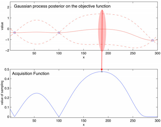
Figure 1.
Illustration of Bayesian Optimization, maximizing an objective function f with a one-dimensional continuous input [20].
2.3. Gaussian Distribution and Gamma Distribution
The Gaussian distribution is used to represent continuous value distributions in discrete values in binomial distributions, such as selecting a coin’s side, and a distribution with an average of 0 and a standard deviation of 1 is called the standard normal distribution.
The Gamma distribution represents the time taken for a total number of Poisson events which occur on average times per unit time, and is used under the normal data distribution assumption. The Poisson distribution is used when the event number N is large and the probability P is low, and is used for discrete distributions. For continuous variables, the Gamma distribution is used [13].
3. Proposed Object Function
An object function is the function to be predicted finally. In this paper, we need to predict the function of the result of the MNIST learning module. In previous papers, Bayesian Optimization (BO) has been used to predict the accuracy by returning accuracy and setting the relationship between this value and learning rate as a function, then setting this as the objective function. However, the problem in the existing studies is that the value varied greatly, even with a small change in the learning rate, due to the sensitivity of the accuracy value. This means that the graph was not stable, as a whole. Therefore, we applied the loss value, which is typically used to evaluate well-training in machine learning.
However, the result was worse than the existing accuracy. The reason for this is that the loss value is usually set to a low value. Also, low loss does not necessarily mean high accuracy. In order to solve this problem, we propose a method that considers the loss value and estimation accuracy, as follows (Equation (6)):
In Equation (6), stands for accuracy, stands for loss, was inserted as the adjusted value in the range from 0 to 1, and log was applied to the function as we could not estimate the range of the loss value. This is because we hope that will have the lowest value and that will have the highest value. For this, we subtract from to determine the satisfied result; note that the result may be negative.
This study is related to the Acquisition Function, rather than the Surrogate Model of BO. In existing Expected Improvement (EI), the distribution of the Surrogate Model (SM) is referred to, and the area expected to have the next highest value is searched for, as shown in Figure 2.
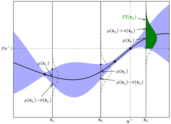
Figure 2.
An example of the region of probable improvement [18].
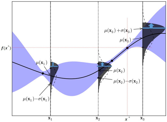
Figure 3.
An example of region of probable improvement using a Gamma Distribution [24].
The maximum observation is . In the overlapping Gaussian, over the dotted line, the dark shaded area can be used as a measure of improvement, . In this model, sampling at is more likely to be improved at , as compared to at . However, using a gamma distribution rather than a Gaussian distribution results in a higher value, which results in better results in the objective function of the MNIST model. In this study, the same method was applied, as follows: Figure 4 shows the test for BO, where it can be seen that the optimal value was found 10 consecutive times. The noise-free object function used in the test was a curve with a paddle point (left) and a local point (right), and The black points in this curve describe the newly discovered location in the test. As shown in Figure 5, it can be confirmed that the sixth saddle point was found in the existing study. In Figure 4, the distance value (left) and the calculation value of EI (right) are shown.
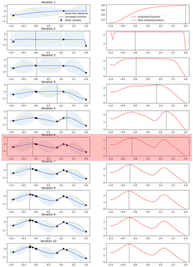
Figure 4.
Tested of Gaussian Process with Gaussian distribution.
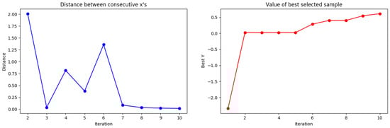
Figure 5.
Tested results of distances and the best selected samples to Gaussian distribution.
In Figure 6, we can see that the fourth highest distance value in the left figure was found to be higher than the local point, following which, we search around the paddle point and find the highest point. Figure 6 and Figure 7 show the results when applying the method presented in this study, from which it can be confirmed that the paddle point was already found in the fourth iteration, unlike the conventional method. In other words, since it proceeds in the form of searching left to right within the entire range, it was easily found that there is a position higher than the local point. The distance calculation for each round can be confirmed to be decreasing flatter than when the Gaussian distribution was used. The reason for measuring the distance is that, the greater the distance from the estimated point, the greater the uncertainty will be. In this regard, it is related to the Exploration–exploitation trade-off. Additionally, in sampling, we can see that the value has been changed from the fourth to the higher value, which shows that the sub-probability between the points in the general GP was passive and, so, the local maximum may be particularly useful in many graphs [18].
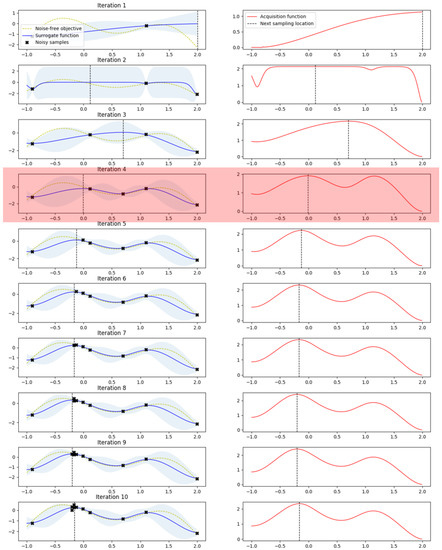
Figure 6.
Tested of Gaussian process with Gamma distribution.
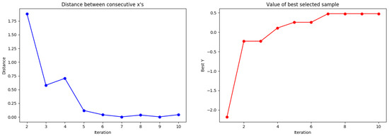
Figure 7.
Tested results of distances and the best selected samples to Gamma distribution.
As shown in Figure 7, at the third time point the actual local point was passed, but it was found that the paddle point was more stable than the existing one. In other words, the proposed method shows that the Gamma distribution can converge faster by using the existing Gaussian process as a method of determining the next measurement point.
4. Experiment on MNIST
We applied grid search, random search, and Bayesian optimization to MNIST and compared the Gaussian Process of Bayesian optimization with the Gaussian and Gamma distributions. In addition, a MNIST model objective function is proposed as a method of applying the loss value and accuracy together in the existing technique. In order to obtain the result quickly, the training data was limited to 500, and the verification data was set to 20%. In other words, the experiment was conducted with the purpose of providing the values for constructing the objective function. The graph part of some programs was detailed in Martin Krasser’s Blog, and the Gaussian Process Regression (GPR) was provided by the scikit-learn package and PyOpt. The detailed conditions of MNIST, which are generally used, are shown in Table 2.
Table 2.
Circumstances of test on MNIST.
Figure 8 shows a graph of the MNIST learning module in a grid method using 100 LRs. Among them, graphs of the accuracy value of the verification data as the y value are shown above, and graphs of the loss value as the y value are shown below. The bounds of LR were set from 0–0.5.
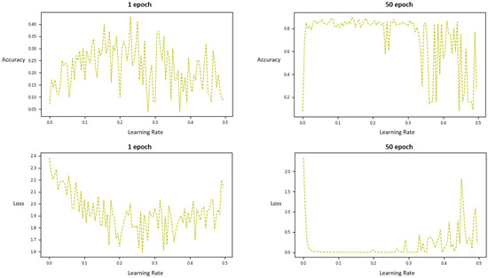
Figure 8.
Estimation graph of objective function for the MNIST model. The 1 epoch and 50 epoch graphs in the top row are objective functions with accuracy as y values, and the two plots in the bottom row show the loss values.
As can be seen from the above Figure 8, a well-trained model indicates the highest accuracy or the lowest loss value. Importantly, there were many local maxima in the graph, and it is important to overcome these local maxima and find the saddle point. Generally, training evaluation in the machine learning module uses the loss value. However, in this study, the estimation accuracy and loss values were considered together, as shown in Figure 9. Figure 8, it shows a graph with as y values for 100 LR values. The highest accuracy is 90 and the corresponding LR value is 0.13. Compared to the case of using only the existing loss value or the accuracy only, it that can be seen that the local maxima disappeared significantly before the LR = 0.2 point. By using two values at the same time, the local maxima of the objective function can be minimized; this makes the objective function easier to estimate.
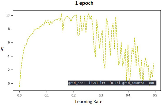
Figure 9.
Estimation graph of objective function to MNIST model using .
Therefore, the method presented in this paper is of great importance, and the results are explained below, based on the accuracy comparison in Section 5 and the comparison using Gaussian distribution and Gamma distribution. In addition, the graphs after LR 0.2 seem problematic. However, if LR shows the highest accuracy at 0.13, it may be excluded; but further research is needed.
Figure 10 shows the results at 1 epoch, using MNIST as the objective function. The left side shows the results of using the Gaussian distribution search and the right side shows the results of using the Gamma distribution search. The purpose of this paper is to estimate the distribution of the objective function of the MNIST module using the minimum number of estimates. Regarding the minimum number of times between the Gaussian and Gamma distribution searches, we could confirm that it had an advantage over the existing results. However, compared with the grid search, existing research has been applied only to the search times, such that a clear comparison between the searching techniques could not be carried out. In this regard, more accurate analysis would be possible if the comparison was made based on accuracy and, thus, the maximum difference value could be compared, with a comparison of when similar accuracy values were derived. In addition, the experiment was conducted by utilizing , as in described Section 3 of this paper. As shown in Figure 10, the accuracy of the proposed method was 47%, and the number of search iterations was the smallest in finding the highest accuracy. The method using the Gaussian distribution search was 39%, and the number of search iterations was nine. Finally, for the grid method, the accuracy was 46% and the number of iterations was 100.
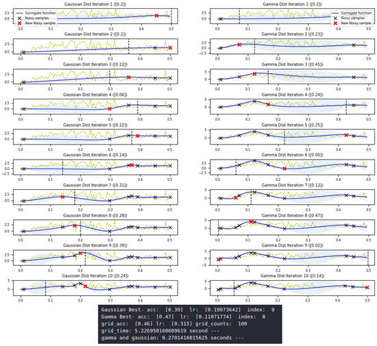
Figure 10.
Comparison of Gaussian distribution and Gamma distribution at 1 epoch. The yellow dashed line shows non-free observations of the objective function f at 300 points; that is, the graph of the y value with an input of 100 x values (grid type) directly for the objective function. The blue line is an estimated graph of the objective function for the x values, which is 10 times sequentially calculated using the Acquisition Function. The red x points represent the final predicted points for each step.
In other words, the number of iterations needed for a similar level of accuracy were lower than the Gaussian distribution search, as the difference of accuracy was 7% and difference in number of iterations was one. In addition, the LR of the proposed method was about 0.11, where grid search showed a result of about 0.32. In this case, it is not clear whether the optimal position of the LR was 0.11 or around 0.32.
As described above, it was found that the Local maximum frequently occurred again after a certain LR value. Considering this, the accurate saddle point could be estimated as 0.11.
Figure 11 shows the results at 50 epochs. For the proposed technique, the accuracy was 94% and the LR was about 0.12; for the Gaussian distribution search, the accuracy was 93% and the LR was about 0.2. In the case of the grid search, the accuracy was 93% and the LR was 0.16. As a result, in the case of grid search, an estimated 100 iterations were required, but the proposed method had similar effects with about only 7 iterations.
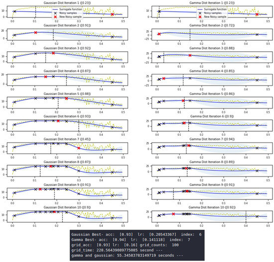
Figure 11.
Comparison of Gaussian distribution search and Gamma distribution search at 50 epochs.
5. Performance Evaluation
In terms of performance evaluation, the evaluation metrics used to measure the predictive performance of the model include the sensitivity, specificity, accuracy, and MCC (mathew correlation coefficient) of the evaluation. TP, FP, TN, and FN are shown as true positive, false positive, true negative, and false negative, respectively. In addition to the following equations, this study evaluates the analysis speed based on the time required for learning to the level that the accuracy is matched based on the number of grids [25].
6. Evaluation
The grid search, Gamma distribution search, and Gaussian distribution search methods were compared to the existing methods (except for random search, as the uncertainty in the method is large). The actual random search method is excellent, in terms of learning speed, but the number of epochs or steps may increase infinitely when learning a lot of data. In particular, the final evaluation was made by comparing the accuracy with and without the added value in Table 3 and Figure 11 and Figure 12.
Table 3.
Comparison of random search, Gaussian distribution search, and Gamma distribution search using 400 traing data set and 100 validation data set.
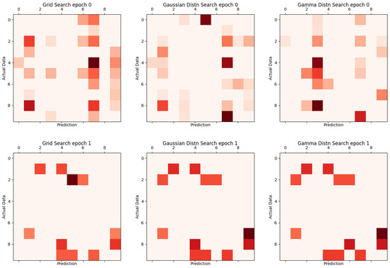
Figure 12.
Existing comparison of grid search, Gaussian distribution search, and Gamma distribution search.
Table 3 shows the comparative evaluation of the existing system and the proposed system. The proposed method can improve the performance by applying in the previous research to derive more convex output value from the objective function. Epoch did not proceed further. Because the evaluated data is the small data, further progression does not affect the accuracy (use small data). However, there is no shortage in comparing the proposed system with the existing system. In other words, it is possible to confirm the high value in terms of accuracy, sensitivity, or specificity.
Figure 12 and Figure 13 are visual representations of the results in Table 3, with the vertical axis representing the actual label and the horizontal axis representing the value of the result inferred from learning. The darker the color, the more inconsistent.
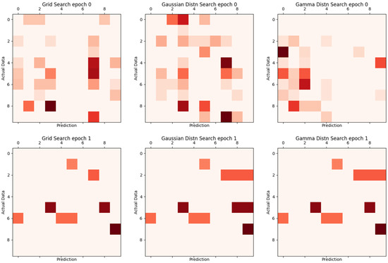
Figure 13.
Proposed comparison of grid search, Gaussian distribution search, and Gamma distribution search.
Table 4 shows the training results using 60,000 training data and 10,000 verification data in units of epoch. From the learning results, it can be seen that the Gamma distn search method shows the maximum in 2 Epoch. This table is not compared with previous studies, but the results were smaller than the current results without . Compared with the general CNN, it shows that the learning accuracy is high. In Table 4, 1 epoch means that is 10 epoch to the same learning model because we try to 12 optimization per 1 epoch. Thus, the above results represent accuracy for a total of 24 epochs. Figure 14 shows the result of Table 4.
Table 4.
Comparison of random search, Gaussian distribution search, and Gamma distribution search using 60,000 traing data set and 10,000 validation data set. Detailed results are in Appendix A.
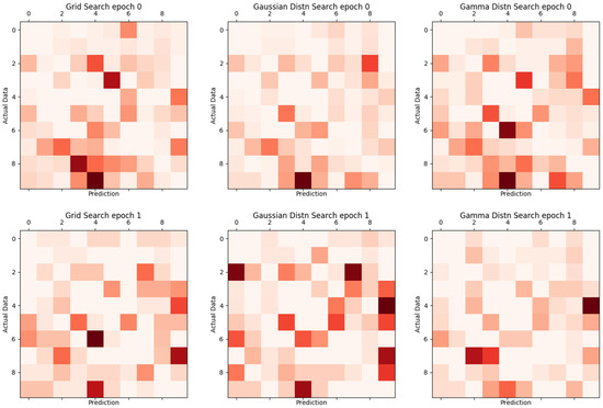
Figure 14.
Proposed comparison of grid search, Gaussian distribution search, and Gamma distribution search.
Table 5 shows the results of examining the increase and decrease for each epoch using CIFAR-10. The model applied the model suggested by keras and shows a learning effect of at a maximum of 50 epochs. This data set was chosen to increase the discrimination of the proposed method regardless of the model. As the result, the method presented in this paper shows that the accuracy increases regardless of the model type, and shows high values of sensitivity and specificity. Figure 15 shows the agreement for each epoch.
Table 5.
Comparison of keras CNN, Gaussian distribution search of keras CNN, and Gamma distribution search of keras CNN using 50,000 traing data set of CIFAR-10 and 10,000 validation data set of CIFAR-10.
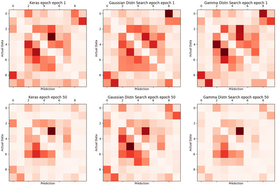
Figure 15.
Proposed comparison of grid search, Gaussian distribution search, and Gamma distribution search.
Table 6 shows the comparison of the grid search, Gaussian distribution search, and Gamma distribution search methods, to which 10 optimizations and 1 epoch were applied. We can see that, the larger the grids, the more the accuracy was increased in the grid search; however, the time required increased accordingly. When comparing the averages, the time required for the Gaussian distribution search and the proposed search were almost unchanged and similar, but the accuracy was more than 7% improved, which was in agreement with that suggested in the previous studies.
Table 6.
Comparison of grid search, Gaussian distribution search and Gamma distribution search, applying 10 counts of optimization and 1 epoch. LT, learning time.
Table 7 describes the comparison of the grid search, Gaussian distribution search, and Gamma distribution search, with 10 optimizations and 50 epochs. In particular, even though the number of grids increased, the accuracy was not affected significantly. Comparing the average for grid size from 100–500, there was a 0.7% difference between the suggested search and the grid search. However, the time of grid search was 729.9 s, and the suggested search took 29.38, which was about 24.8 times faster. Additionally, in comparison with the Gaussian distribution search, it was confirmed that the proposed method showed a 2% increase in accuracy. To confirm the improvement when comparing both the loss value and the accuracy estimate, the experiment was conducted again with 20 optimizations. The results are shown in Table 8.
Table 7.
Comparison of grid search, Gaussian distribution search, and Gamma distribution search, applying 10 counts of optimization and 50 epochs. LT, learning time.
Table 8.
Comparison of grid search, Gaussian distribution search, and Gamma distribution search applying 20 counts of optimization and 50 epochs. LT, learning time; LR, learning rate.
As mentioned earlier, Table 8 will be compared with existing research data, and we will also study LR. It is important to see whether the actual optimized point was a saddle point or not. However, for points obtained by grid search, we can think of them as an approximations to a saddle point. In other words, with high accuracy and similar LR to a saddle point, we can expect to find a more accurate point if we increase the number of optimizations.
Comparing the average values in Table 7, can be used to confirm the overall improvement in learning speed, compared to previous studies. Compared with grid search, the time difference was much higher than the accuracy difference. When looking at the accuracy of time, the existing method was faster and had higher accuracy. Furthermore, the results of the proposed method were higher in accuracy than the Gaussian distribution search. In addition, in the case of LR, the proposed method had a value closer to that of LR of grid search than the Gaussian distribution search; in other words, the proposed search method was superior to the existing systems, in terms of accuracy and required time.
7. Conclusions
At present, Google is indispensable for machine learning, and even more so for AutoML. In view of recent issues, it is expected that AutoML will become pivotal in future machine learning. Variables directly related to AutoML include learning rate, mini-batch size, and normalization coefficients, and these variables have always been created and distributed by the machine trainers. In this regard, when the data set is changed and needs to be retrained, the problems that need to be reviewed for the hyperparameters and the decisions about variables expected by the actual person or guessed are closely related to the time, cost, and performance. For this, unfortunately, a full understanding of the learning parameters, expert experience, and numerous experiments are required. However, if possible, the smart way to solve this problem is to let the machine obtain these parameters for you.
In this study, we attempted to find a solution for the learning rate, among these problems. Therefore, we reviewed the commonly used random search, grid search, and Bayesian optimization methods by applying the well-known MNIST data, and presented a method to apply a Gamma distribution to the acquisition function for Bayesian optimization.
In addition, we presented a method for evaluating the learning rate by using both the accuracy and loss values in the sampling, in order to analyze the distribution of the objective function of the MNIST model.
Although the results of some experiments showed higher values than the existing methods, as seen in the Section 6, it was proved that the proposed search technique presented better results, in most evaluations.
In addition, we can confirm that the result of using the function has a convex distribution; if we can predict a more convex distribution, we can expect to find a more reasonable saddle point. In further research, we will study the construction of the more convex models, among the studies on the values output from the black box.
Author Contributions
Conceptualization, Y.K. and M.C.; methodology, Y.K. and M.C.; software, Y.K.; validation, Y.K. and M.C.; formal analysis, Y.K. and M.C.; investigation, Y.K. and M.C.; resources, Y.K.; data curation, Y.K.; writing—original draft preparation, Y.K.; writing—review and editing, Y.K. and M.C.; visualization, Y.K.; supervision, M.C.; project administration, M.C.; funding acquisition, Y.K. and M.C.
Funding
This research was supported by Basic Science Research Program through the National Research Foundation of Korea (NRF) funded by the Ministry of Education (NRF-2017R1D1A1B03030033).
Acknowledgments
The first draft of the paper was presented in the section “Deep Learning and Application” of The 15th International Conference on Multimedia Information Technology and Applications (MITA2019) held by Korean Multimedia Society(KMMS) and University of Economics and Law(UEL).
Conflicts of Interest
The authors declare no conflict of interest.
Appendix A. Training Progress Detailed Results
| Gamma Distn Search Maximum Acurracy Detail |
| —————-epoch————–(step: 0 ) gamma-bounds: [[1.e-04 5.e-01]]”’ gaussian-bounds: [[1.e-04 5.e-01]] grid-bounds: [[1.e-04 5.e-01]] Gamma Best- acc: [0.9564] lr: [0.15058182] index: 3 Gaussian Best- acc: [0.9575] lr: [0.20195701] index: 3 grid-acc: [0.9562] lr: [0.110078] grid-counts: 100 grid-time: 1525.9515149593353 second — gamma gaussian: 320.44497871398926 seconds — ————————-Gamma———————— accuracy: 0.99128 confusion: 4545.6265772727265 precision: 0.9561963371512057 recall: 0.9560669819496841 mcc: 0.9512168890174788 sensitivity: 0.9560669819496841 specificity: 0.9951604430746006 ————————-Gaussian———————— accuracy: 0.9914999999999999 confusion: 4545.906891110488 precision: 0.9573654579832793 recall: 0.9573670489406423 mcc: 0.9525345363214628 sensitivity: 0.9573670489406423 specificity: 0.9952837099770188 ————————-Grid———————— accuracy: 0.99124 confusion: 4545.906947140898 precision: 0.956117721154721 recall: 0.9558912053696996 mcc: 0.9510239135134221 sensitivity: 0.9558912053696996 specificity: 0.9951402792741156 —————-epoch————–(step: 1 ) gamma-bounds: [[0.06023273 0.21081454]] gaussian-bounds: [[0.0807828 0.28273981]] grid-bounds: [[0.0440312 0.1541092]] Gamma Best- acc: [0.9836] lr: [0.06023273] index: 0 Gaussian Best- acc: [0.9813] lr: [0.0807828] index: 0 grid-acc: [0.9818] lr: [0.06934914] grid-counts: 100 grid-time: 3392.1185035705566 second — gamma gaussian: 308.5484368801117 seconds — ————————-Gamma———————— accuracy: 0.99672 confusion: 4562.803546984866 precision: 0.9835683589709514 recall: 0.9835058725009371 mcc: 0.9817028741071395 sensitivity: 0.9835058725009371 specificity: 0.9981785294864007 ————————-Gaussian———————— accuracy: 0.99626 confusion: 4545.908262967948 precision: 0.981316407524821 recall: 0.9810898959265562 mcc: 0.9791059831360185 sensitivity: 0.9810898959265562 specificity: 0.997922830382359 ————————-Grid———————— accuracy: 0.9963599999999999 confusion: 4545.908146741083 precision: 0.981879115324593 recall: 0.9815012472351764 mcc: 0.9796568657792945 sensitivity: 0.9815012472351764 specificity: 0.9979768937659553 —————-epoch————–(step: 2 ) gamma-bounds: [[0.02409309 0.08432582]] gaussian-bounds: [[0.03231312 0.11309592]] grid-bounds: [[0.02773966 0.0970888 ]] Gamma Best- acc: [0.9823] lr: [0.02409309] index: 0 Gaussian Best- acc: [0.9821] lr: [0.03550456] index: 6 grid-acc: [0.9783] lr: [0.02982013] grid-counts: 100 grid-time: 5223.958828687668 second — gamma gaussian: 343.67405676841736 seconds — ————————-Gamma———————— accuracy: 0.9964599999999999 confusion: 4545.632518181818 precision: 0.9823391951737168 recall: 0.982118716591801 mcc: 0.9802569569051883 sensitivity: 0.982118716591801 specificity: 0.9980324760992 ————————-Gaussian———————— accuracy: 0.99642 confusion: 4545.635281241946 precision: 0.9820085701478038 recall: 0.9819438346460284 mcc: 0.9799852874924644 sensitivity: 0.9819438346460284 specificity: 0.9980115536490326 ————————-Grid———————— accuracy: 0.99566 confusion: 4546.037013372861 precision: 0.9781982768860729 recall: 0.978143086587466 mcc: 0.9757536738243268 sensitivity: 0.978143086587466 specificity: 0.9975895338444459 —————-epoch————–(step: 3 ) gamma-bounds: [[0.00963724 0.03373033]] gaussian-bounds: [[0.01420183 0.04970639]] grid-bounds: [[0.01192805 0.04174818]] Gamma Best- acc: [0.9813] lr: [0.02185781] index: 2 Gaussian Best- acc: [0.9812] lr: [0.0207021] index: 2 grid-acc: [0.9837] lr: [0.01312086] grid-counts: 100 grid-time: 7069.49636721611 second — gamma gaussian: 350.1422553062439 seconds — ————————-Gamma———————— accuracy: 0.99626 confusion: 4545.63475035308 precision: 0.9812261638722205 recall: 0.9811773662104988 mcc: 0.9791226848339004 sensitivity: 0.9811773662104988 specificity: 0.9979225414069898 ————————-Gaussian———————— accuracy: 0.9962399999999999 confusion: 4545.635264046948 precision: 0.9810652055934064 recall: 0.9810538040503666 mcc: 0.9789703109590817 sensitivity: 0.9810538040503666 specificity: 0.9979120643565299 ————————-Grid———————— accuracy: 0.99674 confusion: 4546.036578721596 precision: 0.9836110493048572 recall: 0.9834916677629966 mcc: 0.9817387961353237 sensitivity: 0.9834916677629966 specificity: 0.998189550424739 |
References
- Zhang, Z.; Jiang, T.; Li, S.; Yang, Y. Automated feature learning for nonlinear process monitoring–An approach using stacked denoising autoencoder and k-nearest neighbor rule. J. Process Control 2018, 64, 49–61. [Google Scholar] [CrossRef]
- Zoph, B.; Le, Q.V. Neural architecture search with reinforcement learning. arXiv 2016, arXiv:1611.01578. [Google Scholar]
- Krizhevsky, A.; Sutskever, I.; Hinton, G.E. Imagenet classification with deep convolutional neural networks. In Proceedings of the Advances in Neural Information Processing Systems 25, Neural Information Processing Systems(NIPS), Lake Tahoe, NV, USA, 3–8 December 2012; pp. 1097–1105. [Google Scholar]
- Jones, D.R.; Schonlau, M.; Welch, W.J. Efficient global optimization of expensive black-box functions. J. Glob. Optim. 1998, 13, 455–492. [Google Scholar] [CrossRef]
- Bergstra, J.; Bengio, Y. Random search for hyper-parameter optimization. J. Mach. Learn. Res. 2012, 13, 281–305. [Google Scholar]
- Bergstra, J.S.; Bardenet, R.; Bengio, Y.; Kégl, B. Algorithms for hyper-parameter optimization. In Proceedings of the Advances in Neural Information Processing Systems 24, Neural Information Processing Systems(NIPS), Granada, Spain, 12–17 December 2011; pp. 2546–2554. [Google Scholar]
- Guo, B.; Hu, J.; Wu, W.; Peng, Q.; Wu, F. The Tabu Genetic Algorithm A Novel Method for Hyper-Parameter Optimization of Learning Algorithms. Electronics 2019, 8, 579. [Google Scholar] [CrossRef]
- Je, S.M.; Huh, J.H. An Optimized Algorithm and Test Bed for Improvement of Efficiency of ESS and Energy Use. Electronics 2018, 7, 388. [Google Scholar] [CrossRef]
- Monroy, J.; Ruiz-Sarmiento, J.R.; Moreno, F.A.; Melendez-Fernandez, F.; Galindo, C.; Gonzalez-Jimenez, J. A semantic-based gas source localization with a mobile robot combining vision and chemical sensing. Sensors 2018, 18, 4174. [Google Scholar] [CrossRef] [PubMed]
- Snoek, J.; Larochelle, H.; Adams, R.P. Practical bayesian optimization of machine learning algorithms. In Proceedings of the Advances in Neural Information Processing Systems 25, Neural Information Processing Systems(NIPS), Lake Tahoe, NV, USA, 3–8 December 2012; pp. 2951–2959. [Google Scholar]
- Calandra, R.; Peters, J.; Rasmussen, C.E.; Deisenroth, M.P. Manifold Gaussian processes for regression. In Proceedings of the 2016 International Joint Conference on Neural Networks, Vancouver, BC, Canada, 24–29 July 2016; pp. 3338–3345. [Google Scholar]
- Bergstra, J.; Yamins, D.; Cox, D.D. Making a science of model search: Hyperparameter optimization in hundreds of dimensions for vision architectures. In Proceedings of the 30th International Conference on Machine Learning, Atlanta, GA, USA, 17–19 June 2013; pp. 115–123. [Google Scholar]
- DeGroot, M.H.; Schervish, M.J. Probability and Statistics; Pearson Education Limited: London, UK, 2014; pp. 302–325. [Google Scholar]
- Törn, A.; Žilinskas, A. Global Optimization; Springer: Berlin, Germany, 1989. [Google Scholar]
- Mongeau, M.; Karsenty, H.; Rouzé, V.; Hiriart-Urruty, J.B. Comparison of public-domain software for black-box global optimization. Optim. Methods Softw. 1998, 13, 203–226. [Google Scholar] [CrossRef]
- Liberti, L.; Maculan, N. Global Optimization: From Theory to Implementation; Springer Optimization and Its Applications; Springer: Berlin, Germany, 2006. [Google Scholar]
- Zhigljavsky, A.; Žilinskas, A. Stochastic Global Optimization; Springer Optimization and Its Applications; Springer: Berlin, Germany, 2007. [Google Scholar]
- Brochu, E.; Cora, V.M.; De Freitas, N. A tutorial on Bayesian optimization of expensive cost functions, with application to active user modeling and hierarchical reinforcement learning. arXiv 2010, arXiv:1012.2599. [Google Scholar]
- Mockus, J. Application of Bayesian approach to numerical methods of global and stochastic optimization. J. Glob. Optim. 1994, 4, 347–365. [Google Scholar] [CrossRef]
- Frazier, P.I. A tutorial on bayesian optimization. arXiv 2018, arXiv:1807.02811. [Google Scholar]
- Jones, D.R. A taxonomy of global optimization methods based on response surfaces. J. Glob. Optim. 2001, 21, 345–383. [Google Scholar] [CrossRef]
- Lizotte, D. Practical Bayesian Optimization. Ph.D. Thesis, University of Alberta, Edmonton, AB, Canada, 2008. [Google Scholar]
- Pelikan, M.; Goldberg, D.E.; Cantú-Paz, E. BOA: The bayesian optimization algorithm. In Proceedings of the 1st Annual Conference on Genetic and Evolutionary Computation, Orlando, FL, USA, 13–17 July 1999; Volume 1, pp. 525–532. [Google Scholar]
- Kim, Y.; Chung, M. An Approch of Hyperparameter Optimization using Gamma Distribution. In Proceedings of the 15th International Conference on Multimedia Information Technology and Applications, University of Economics and Law, Ho chi minh, Vietnam, 27 June–1 July 2019; Volume 1, pp. 75–78. [Google Scholar]
- Le, N.Q.K.; Huynh, T.T.; Yapp, E.K.Y.; Yeh, H.Y. Identification of clathrin proteins by incorporating hyperparameter optimization in deep learning and PSSM profiles. J. Comput. Methods Prog. Biomed. 2019, 177, 81–88. [Google Scholar] [CrossRef] [PubMed]
© 2019 by the authors. Licensee MDPI, Basel, Switzerland. This article is an open access article distributed under the terms and conditions of the Creative Commons Attribution (CC BY) license (http://creativecommons.org/licenses/by/4.0/).