Real-Time Detection and Recognition of Multiple Moving Objects for Aerial Surveillance

Abstract

Detection of moving objects by unmanned aerial vehicles (UAVs) is an important application in the aerial transportation system. However, there are many problems to be handled such as high-frequency jitter from UAVs, small size objects, low-quality images, computation time reduction, and detection correctness. This paper considers the problem of the detection and recognition of moving objects in a sequence of images captured from a UAV. A new and efficient technique is proposed to achieve the above objective in real time and in real environment. First, the feature points between two successive frames are found for estimating the camera movement to stabilize sequence of images. Then, region of interest (ROI) of the objects are detected as the moving object candidate (foreground). Furthermore, static and dynamic objects are classified based on the most motion vectors that occur in the foreground and background. Based on the experiment results, the proposed method achieves a precision rate of 94% and the computation time of 47.08 frames per second (fps). In comparison to other methods, the performance of the proposed method surpasses those of existing methods.

1. Introduction

There has been increased worldwide interest in unmanned aerial vehicles (UAVs) used for surveillance in recent years due to their high mobility and flexibility. In general, the UAV with a camera attached for surveillance flying over the mission area can be controlled manually by an operator or automatically by using computer vision. One of the most important tasks of aerial surveillance is the detection of moving objects that can be used to convey essential information in images, such as pedestrian detection and tracking [1,2,3], vehicle detection and tracking [4,5], object counting [6], estimation and recognition of object activity [7,8,9], human and vehicle interactions [10], intelligent transportation systems [11,12], traffic management [13,14], and autonomous robot navigation [15,16].

Several studies have proposed some methods to detect moving objects using stationary cameras, such as Gaussian Mixture Model (GMM) [17], Bayesian background model [18], Markov Random Field (MRF) [19,20], and frame differences [21,22]. These methods extract and identify moving objects by seeking the changes in pixels in each frame. However, these techniques rely on static pixels in the images and are not suitable for processing images from moving cameras that have dynamic pixels. Therefore, stationary cameras limit the application of image processing on videos from moving cameras, e.g., aerial vehicles, mobile robots, and handheld cameras. Thus, the problem for detecting moving objects using a moving camera attracted the attention of researchers in recent years [23].

Detecting moving objects using UAVs has many difficulties to implement in real time and in real environments. These difficulties include camera movements, dynamic background, abrupt motion of the objects or camera, rapid illumination changes, camouflage of stationary objects as moving objects, moving object appearance changes, noise from low-quality images, and so on. Several approaches have been proposed to detect moving objects by moving cameras using object segmentation techniques. Saif et al. [24] presented a dynamic motion model using moment invariant and segmentation which extracts one frame in one second but it is not fast enough for the real-time detection. Their result has some false detection, such as a parked car recognized as a moving object. Maier et al. [25] used the deviations between all pixels of the anticipated geometry of two or more consecutive frames to distinguish moving and static objects, but the result depended on the accuracy of the optical flow calculation and the amount of radial distortion. Kalantar et al. [26] proposed a moving object detection framework without explicitly overlaying frame pairs, where each frame is segmented into regions and subsequently represented as a regional adjacency graph (RAG).

In our propose method, we do not only want to achieve the accuracy of the moving objects detection using a moving camera but also to do it in real-time processing. Some previous studies used an optical flow schemes approach to define the movement path of pixels that are tracked on two consecutive frames. Wu et al. [27] used a coarse-to-fine threshold scheme on particle trajectories in the sequence of images to detect moving objects. The background movement is subtracted using the adaptive threshold method to get fine foreground segmentation. Then, mean-shift segmentation is used to refine the detected foreground. Cai et al. [28] combined procedures of the brightness constancy relaxation and intensity normalization within the optical flow to extract the moving objects in the background based on the growing region of the velocity field. In this case, the images are obtained from the robot competition arena which has a homogeneous background. Minaeian et al. [29] used the foreground estimation to segment moving targets through the integration of spatiotemporal differences and local motion history. However, these previous methods did not adequately prove reliability in real-time processing.

This paper proposes a method for detecting multiple moving objects from the sequence of images taken by a UAV which can be applied for real-time applications. The detection and recognition are performed through this method for different objects, such as people and cars. In addition, the image sequences to be tested by this method may contain a complex background. This paper proposes a reliable method for object detection in images where the processing time to get the foreground is shorter than that of segmentation method employed in previous studies [24,25,26]. Aerial image stabilization is proposed to reduce the mixing of camera and object movements, where the background moves due to the camera movement and the foreground moves due to camera and object movement. Furthermore, the unwanted camera movements make the motion vectors field estimation between two consecutive frames incompatible with the actual situation. This situation differentiates the direction of the motion vectors of static objects from the background, even though the objects are a part of the background. Thus, the static objects tend to be recognized as moving objects. To solve such problems, the proposed method provides the motion vectors classification to distinguish static and dynamic (moving) objects.

The remainder of the paper is organized as follows. Section 2 introduces materials and the main algorithm. Section 3 illustrates performance results using multiple videos taken from a UAV. Finally, conclusions are drawn in Section 4.

2. Materials and Method

2.1. Materials

The experiment was executed using Visual Studio C++ in the 3.40 GHz CPU with 8 GB RAM. The performance of the proposed method is evaluated using three types of aerial image sequences (action1, action2, and action3) obtained from the UCF (http://crcv.ucf.edu/data/UCF_Aerial_Action.php) aerial action dataset with the resolution of 960 × 540. These image sequences were recorded at different flying altitudes ranging from 400–450 feet. Action1.mpg and action2.mpg were taken by the UAV at similar altitudes, where people and cars are the main objects in the image. Action3.mpg was taken at a higher altitude than other videos, so the objects look smaller when compared to other videos.

2.2. The Proposed Method

The challenge to the moving object detection by a moving camera is obvious. The application of the proposed framework can be used to distinguish the foreground from a dynamic background into a simpler formulation. The systematic approach starts with image stabilization to reduce unwanted movement in the sequence of images. The unwanted movements are the motion of the camera as well as any vibration of the UAV. Inaccuracies in motion compensation can cause failure on the estimation of the background and foreground pixels [30]. However, despite using image stabilization, motion vectors in the static objects (background) and moving objects (foreground) are still difficult to distinguish.

Additionally, in order to detect several moving objects with different sizes and speeds we require the correct calculation of motion vector fields. Furthermore, static and dynamic objects are distinguished based on their movement direction (MD). There are two kinds of MD to be estimated: The direction of the object’s movement (foreground) and the direction of the background’s movement. It should be noted that the background motion is affected by the camera’s movement. Figure 1 shows an illustration of the movement of a UAV affecting camera movement. The background movement corresponding to the motion of a moving camera is affected by UAV movements on the yaw, pitch, and roll axis. So, efficient affine transformation is needed.

Figure 2 shows an overview of the structure of the system. The algorithm consists of three steps to accomplish the main task: Step 1 is the aerial image stabilization, step 2 is the object detection and recognition, and step 3 is the classification of the motion vectors. The proposed algorithm handles each frame for the moving objects detection and recognition so that it can be used in real-time applications with online image processing.

Step 1: Image stabilization is performed to handle unstable UAV platforms. This step aligns each frame with the adjacent frame in a sequence of aerial images to eliminate the effect of camera movement. This stabilization method consists of motion estimation and compensation. We used the methods of speeded-up robust features (SURF) [31,32,33] and affine transformation [34] to estimate the camera movement based on the position of features which are similar between the previous (t − 1) and current (t) frames. Then use the Kalman filter [35,36] to overcome the changes in frame position due to UAV movement such that the camera movement is compensated for each frame. This image transformation is applied to the frame t, so it affect the results of MD in the background and foreground.

Step 2: People and cars are detected in the images as the moving objects candidates or foreground. In this step, Haar-like features [37] and cascade classifiers [38,39] are used to detect and recognize the objects in the images and determine the region of interest (ROI) for the objects. This is followed by labeling the background and foreground.

Step 3: Calculate the motion vectors from two consecutive images based on the dense optical flow [40]. Background modeling is sometimes incompatible with actual camera movements due to UAV movements and camera transitions. It is noted that Step 1 makes the MD between static and dynamic objects clearer to be distinguished. MD is specified as the value of a highly repetitive motion vector in frame t, which is calculated in the background and each foreground. If the foreground has the same MD as the background, then the object is omitted from the foreground. Thus, the final result is the ROI in the image showing the moving objects.

The details of each step are explained as follows.

2.3. Step 1: Aerial Image Stabilization

This step uses an affine motion model to handle rotation, scaling, and translation. The affine model can be used to estimate movement between frames under certain conditions in the scene [41,42]. For every two successive frames, the previous frame is defined as $f(t-1)$ and the current frame is defined as $f(t)$. In order to reduce the computation time, let the image size be reduced to 75% of the original size and the color is changed into a gray-scale, where $\widehat{f}(t)$ denotes the new image with the above size and color of $f(t)$. The local features on each frame are found using SURF [31] as the feature detector and descriptor. SURF uses an integral image [43] to compute different box filters to detect feature points in the image. If $f(t)$ is an input image and $f_{(x,y)}(t)$ is the pixel value of the location (x,y) at $f(t)$, the value $P(i,j,t)$ is defined as

$$P(i,j,t)={\displaystyle \sum _{x=0}^{x\le i}{\displaystyle \sum _{y=0}^{y\le j}{f}_{(x,y)}\left(t\right)}}.$$

(1)

Haar wavelet [30] corresponding to d_x and d_y are calculated in the x-direction and y-direction, respectively, around each feature point to form a descriptor vector presented as

$$v=({\displaystyle \sum d_x,}{\displaystyle \sum d_y,}{\displaystyle \sum \left|d_x\right|,}{\displaystyle \sum \left|d_y\right|)}.$$

(2)

Then, a 4 × 4 array with each vector having four orientations is constructed and centered on the feature point. Therefore, there will be a total of 64-length vectors for each feature point.

Fast Library for Approximate Nearest Neighbor (FLANN) [44] is used to select a set of feature point pairs between $\widehat{f}(t-1)$ and $\widehat{f}(t)$. Then, the minimum distance for all pairs of feature points is calculated using the Euclidean distance. The matching pair is determined as a feature point pair with a distance less than 0.6. If the total number of matching pairs are more than three, then the selected feature points are used for the next step. Otherwise, the previous trajectory is used as an estimate of the current movement.

In homogenous coordinates, the relationship between a pair of feature points in the $\widehat{f}(t-1)$ and $\widehat{f}(t)$ is given by

$$\left[\begin{array}{c}x(t)\\ y(t)\end{array}\right]=H\left[\begin{array}{c}x(t-1)\\ y(t-1)\\ 1\end{array}\right],$$

(3)

where H is the homogeneous affine matrix given by

$$H=\left[\begin{array}{c}\begin{array}{ccc}1+a_{11}& a_{12}& T_x\end{array}\\ \begin{array}{ccc}{a}_{21}& 1+a_{22}& T_y\end{array}\end{array}\right],$$

(4)

where a_ij is the parameter from the rotation angular θ, T_x, and T_y are parameters of the translation T on the x-axis and y-axis, respectively. An affine matrix can be represented as a least squares problem by

$$\begin{array}{c}L=mh,\\ L={\left[\begin{array}{ccccc}x(1{)}^{\prime }& y(1{)}^{\prime }& \dots & x(\overline{q}{)}^{\prime }& y(\overline{q}{)}^{\prime }\end{array}\right]}^T,\\ m={\left[\begin{array}{ccccc}{M}_0(1)& M_1(1)& \dots & M_0(\overline{q})& M_1(\overline{q})\end{array}\right]}^T,\\ h={\left[\begin{array}{ccccc}1+a_{11}& a_{12}& T_x& 1+a_{21}& \begin{array}{cc}{a}_{22}& T_y\end{array}\end{array}\right]}^T,\end{array}$$

(5)

where $q=1,\dots ,\overline{q}$ is the number order of features, $M_0(q)=\left(\begin{array}{ccc}\begin{array}{ccc}\begin{array}{cc}x(q)& y(q)\end{array}& 1& 0\end{array}& 0& 0\end{array}\right)$, and $M_1(q)=\left(\begin{array}{ccc}\begin{array}{ccc}\begin{array}{cc}0& 0\end{array}& 0& x(q)\end{array}& y(q)& 1\end{array}\right)$.

The optimal estimation h in Equation (5) can be found by using Gaussian elimination to minimize Root Mean Squared Errors (RMSE) calculated by

$$RMSE=\frac{1}{Q}\Vert L-m{h}^{\prime }\Vert =\sqrt{\frac{{\displaystyle \sum _{q=1}^Q{\left(L_q-{\left(m{h}^{\prime }\right)}_q\right)}^2}}{Q^2}}.$$

(6)

Because the affine transform cannot represent the three-dimensional motion which occurs in the image, the outliers are generated in motion estimation. To solve this problem, Random Sample Consensus (RANSAC) [45] is used to filter outliers during the estimation.

Next, the translation and rotation trajectories are compensated to generate a new set of transformations for each frame using the Kalman filter. The Kalman filter consists of two essential parts, prediction and measurement correction. The prediction step estimates the state of the trajectory $\widehat{z}(t)=\left[T_x(t),T_y(t),\widehat{\theta }(t)\right]$ at $\widehat{f}(t)$ as

$$\widehat{z}(t)=z(t-1),$$

(7)

where the initial state is defined by $z(0)=\left[0,0,0\right]$ and the error covariance can be estimated by

$$\widehat{e}(t)=e(t-1)+{\mathsf{\Omega }}_p,$$

(8)

where the initial error covariance is defined by $e(0)=\left[1,1,1\right]$ and ${\mathsf{\Omega }}_p$ is the noise covariance of the process. Optimum Kalman gain can be computed as follows

$$K(t)=\frac{\widehat{e}(t)}{\widehat{e}(t)+{\mathsf{\Omega }}_m},$$

(9)

where ${\mathsf{\Omega }}_m$ is the noise covariance of the measurement. The error covariance can be compensated by

$$e(t)=\left(1-K(t)\right)\widehat{e}(t).$$

(10)

Then, the measurement correction step compensates the trajectory state at $\widehat{f}(t)$, which can be computed as

$$z(t)=z(t)+K(t)\left(\mathsf{\Gamma }(t)-z(t)\right),$$

(11)

where the new state contains the compensated trajectory defined by $z(t)=\left[{T^{\prime }}_x(t),{T^{\prime }}_y(t),{\theta }^{\prime }(t)\right]$ and $\mathsf{\Gamma }(t)$ is the accumulation of the trajectory measurement that can be calculated as follows

$$\mathsf{\Gamma }(t)={\displaystyle \sum _{\tau =1}^{t-1}\left[\left({\overline{T}}_x(\tau )+T_x(t)\right),\left({\overline{T}}_x(\tau )+T_x(t)\right),\left(\overline{\theta }(\tau )+\theta (t)\right)\right]}=\left[{\mathsf{\Gamma }}_x(t),{\mathsf{\Gamma }}_y(t),{\mathsf{\Gamma }}_{\theta }(t)\right].$$

(12)

Therefore, a new trajectory can be obtained by

$$\left[{\overline{T}}_x\left(t\right),{\overline{T}}_y\left(t\right),\overline{\theta }\left(t\right)\right]=\left[T_x(t),T_y(t),\theta (t)\right]+\left[{\sigma }_x(t),{\sigma }_y(t),{\sigma }_{\theta }(t)\right],$$

(13)

where ${\sigma }_x\left(t\right)={T^{\prime }}_x\left(t\right)-{\mathsf{\Gamma }}_x\left(t\right)$, ${\sigma }_y\left(t\right)={T^{\prime }}_y\left(t\right)-\mathsf{\Gamma }\left(t\right)$, and ${\sigma }_{\theta }\left(t\right)={\theta }^{\prime }\left(t\right)-{\mathsf{\Gamma }}_{\theta }\left(t\right)$.

Then, warp $f(t)$ is in the new image plane and let us apply the new trajectory in Equation (13) to get the transformation $\overline{f}(t)$ in the current frame

$$\overline{f}(t)=f(t)\left[\begin{array}{cc}\mathsf{\Phi }(t)\cos \overline{\theta }(t)& -\mathsf{\Phi }(t)\sin \overline{\theta }(t)\\ \mathsf{\Phi }(t)\sin \overline{\theta }(t)& \mathsf{\Phi }(t)\cos \overline{\theta }(t)\end{array}\right]+\left[\begin{array}{c}{\overline{T}}_x(t)\\ {\overline{T}}_y(t)\end{array}\right],$$

(14)

where $\mathsf{\Phi }(t)$ is a scale factor computed by

$$\mathsf{\Phi }(t)=\frac{\cos \overline{\theta }(t)}{\cos \left({\tan }^{-1}\left(\frac{\sin \overline{\theta }(t)}{\cos \overline{\theta }(t)}\right)\right)(t)}.$$

(15)

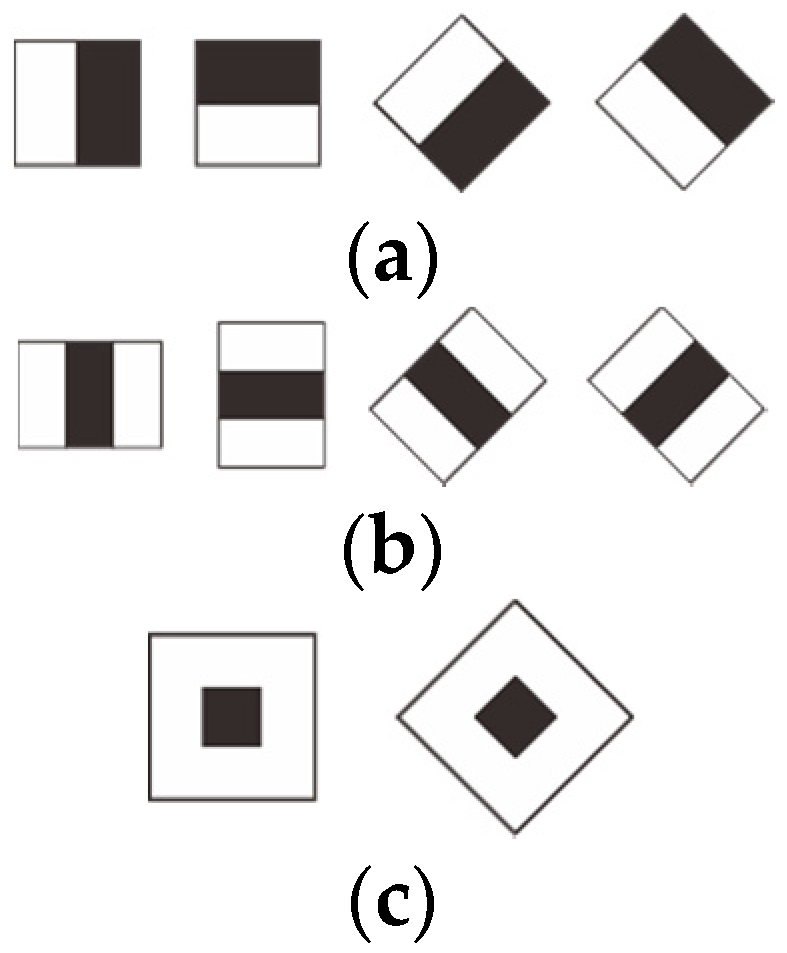
2.4. Step 2: Object Detection and Recognition

In this step, the background and foreground are determined in each frame that has been transformed in Step 1. The foreground is made up of the moving object candidates, which are people and cars, in the image. The foreground is detected and recognized using Haar-like features and a boosted cascade of classifiers with training and detection stages. The basic idea behind Haar-like features is to detect objects of various sizes in the images. Figure 3 shows the template of the Haar-like features where each feature consists of two or three adjacent rectangular groups and can be scaled up or down. The pixel intensity values in the white and black groups are accumulated separately. So, the distinction between adjacent groups gives light and dark regions. Therefore, Haar-like features are suitable for defining information in images to find objects on different scales in which some simple patterns are used to identify the existence of objects.

The Haar-like feature value is calculated as the weighted sum of the pixel gray level values which are summed over the black rectangle and the entire feature area. Then, an integral image [41] is used to minimize the number of array references in the sum of the pixels in a rectangular area of an image. Figure 4a,b show the example of the main objects to be selected. Figure 4c shows the example of the additional objects to be selected which are non-moving objects, i.e., road signs, fences, boxes, road patterns, grass patterns, power lines, roadblocks, and so on. This additional object has the purpose to reduce false detection where the type of object often tends to be recognized as foreground. Negative images are the images of landscapes and roads taken by a UAV without containing cars or people. In this study, the minimum and maximum sizes of positive images to be trained are 16 × 35 and 136 × 106, respectively.

The AdaBoost algorithm [46] is used to combine features of the selected classifier. A classifier is chosen as the threshold to determine the best classification function for each feature. A training sample is set as $\left({\alpha }_{\mathrm{s}},{\beta }_{\mathrm{s}}\right)$, $s=1,2,\dots ,N$, where ${\beta }_s=0,\mathrm{or}1$ for negative or positive labels, respectively, and it is the class label for the sample ${\alpha }_s$. Each sample is converted to a gray-scale then scaled down to the base resolution of the detector. The AdaBoost algorithm creates a weight vector which is distributed over all training samples in the iteration. The initial weight vector for all samples $\left({\alpha }_1,{\beta }_1\right),\dots ,({\alpha }_N,{\beta }_N)$ is set as ${\omega }_1(s)=\raisebox{1ex}{$1$}\!\left/ \!\raisebox{-1ex}{$N$}\right.$. The error associated with the selected classifier is evaluated as

$${\epsilon }_i={\displaystyle \sum _{s=1}^N{\omega }_i(s),\mathrm{if}\left|{\lambda }_i({\alpha }_s)\ne {\beta }_s\right|}.$$

(16)

The ${\lambda }_i({\alpha }_s)=0,\mathrm{or}1$ is a selected classifier for negative or positive labels, respectively, and $i=1,2,\dots ,I$ is the iteration number. The selected classifier is used to update the weight vector as

$$\begin{array}{l}{\omega }_{i+1}(s)={\omega }_i(s){\delta }_i^{1-r_s}\\ \mathrm{where}{r}_s=\{\begin{array}{l}0,\mathrm{if}{\alpha }_s\mathrm{classified}\mathrm{correctly},\\ 1,\mathrm{otherwise}\end{array}\end{array}$$

(17)

and ${\delta }_i$ is the weighting parameter set by

$${\delta }_i=\frac{{\epsilon }_i}{1-{\epsilon }_i}.$$

(18)

The final classifier stage $W(\alpha )$ is the labeled result of each region represented as

$$W(\alpha )=\{\begin{array}{l}1,\mathrm{if}{\displaystyle \sum _{i=1}^I\left[\log \left(\frac{1}{{\delta }_i}\right)\times {\lambda }_i(\alpha )\right]}\ge \frac{1}{2}{\displaystyle \sum _{i=1}^I\log \left(\frac{1}{{\delta }_i}\right).}\\ 0,\mathrm{otherwise}\end{array}$$

(19)

Figure 5 shows a sub-window that slides over the image to identify the region containing the object. The region is labeled at each classifier stage either as positive (1) or negative (0). The classifier passes to the next stage if the region is labeled as positive, which means that the region is recognized as an object. Otherwise, the region is labeled as negative and is rejected. The final stage shows the region of the moving object candidates. The region of the non-moving object is not to be displayed in the image and is used to evaluate the detected object. If the region of a moving object candidate is the same as the non-moving object, then the region is eliminated as a foreground. Let the n-th foreground region be represented as

$$Obj[n]=\left[(x_{\min }(n),y_{\min }(n)),(x_{\max }(n),y_{\max }(n))\right],$$

(20)

where $(x_{\min }(n),y_{\min }(n))$ and $(x_{\max }(n),y_{\max }(n))$ are the minimum and maximum positions of the rectangular foreground pixel locations, respectively.

False detection of the moving object candidates is eliminated immediately using a comparison of the region with non-moving objects. This will speed up the computation time in the next step.

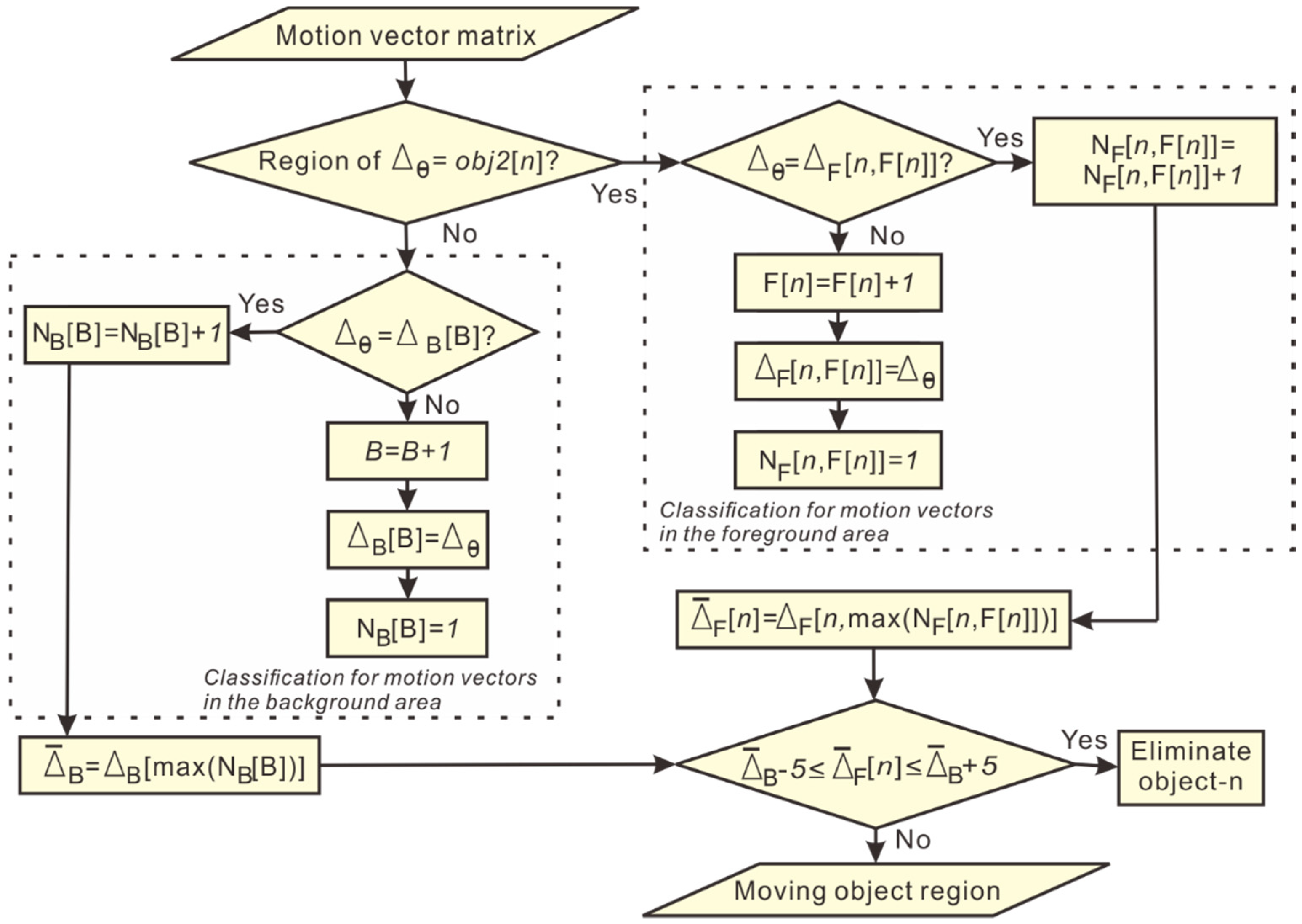
2.5. Step 3: Motion Vector Classification

The Farneback optical flow [40] is adopted to obtain motion vectors of two consecutive images. The Farneback optical flow uses a polynomial expansion to provide high speed and accuracy for field estimation. Suppose there is a 10 × 10 window G(j) and the pixel j is chosen inside the window. By using polynomial expansion, each pixel in G(j) can be approximated by a polynomial so called “local coordinate system” at $f(t-1)$ which can be computed as follows

$$f_{lcs}^p(t-1)=p^{T}A(t-1)p+b^T(t-1)p+c(t-1),$$

(21)

where p is a vector, $A(t-1)$ is a symmetric matrix, $b(t-1)$ is a vector, and $c(t-1)$ is a scalar. The local coordinate system at $f(t)$ can be defined by

$$f_{lcs}^p(t)=p^{T}A(t)p+b^T(t)p+c(t).$$

(22)

Then, a new signal is constructed at $f(t)$ by a global displacement $\Delta \left(t\right)$ as $f_{lcs}^p(t)=f_{lcs}^{p-\Delta (t)}\left(t-1\right)$. The relation between the local coordinate systems of two input images will be

$$\begin{array}{cc}{f}_{lcs}^p(t)& ={(p-\Delta (t))}^{T}A(t-1)(p-\Delta (t))+b^T(t-1)(p-\Delta (t))+c(t-1)\hfill \\ & =p^{T}A(t-1)p^T+{(b(t-1)-2A(t-1)\Delta (t))}^{T}p+{\Delta }^T(t)A(t-1)\Delta (t)-b^T(t-1)\Delta (t)+c(t-1)\hfill \end{array}$$

(23)

The coefficients can be equated in Equations (22) and (23) as

$$A\left(t\right)=A\left(t-1\right),$$

(24)

$$b\left(t\right)=b\left(t-1\right)-2A\left(t-1\right)\Delta \left(t\right),$$

(25)

and

$$c\left(t\right)=\Delta \left(t\right)\left({\Delta }^T\left(t\right)A\left(t-1\right)-b^T\left(t-1\right)\right)+c\left(t-1\right).$$

(26)

Therefore, the total displacement with the extraction in the ROI can be solved by

$$\Delta \left(t\right)=-\frac{1}{2}{A}^{-1}\left(t-1\right)\left(b\left(t\right)-b\left(t-1\right)\right).$$

(27)

The displacement in Equation (27) is a translation from each corresponding ROI consisting of the x-axis $\left({\Delta }_x\left(t\right)\right)$ and y-axis $\left({\Delta }_y\left(t\right)\right)$, so the angular value of the motion vector can be calculated by

$${\Delta }_{\theta }\left(t\right)={\tan }^{-1}\left(\frac{{\Delta }_{\left(x+1,y\right)}\left(t\right)-{\Delta }_{\left(x-1,y\right)}\left(t\right)}{{\Delta }_{\left(x,y+1\right)}\left(t\right)-{\Delta }_{\left(x,y-1\right)}\left(t\right)}\right)\times \frac{180}{\pi }.$$

(28)

Since the motion vector is calculated for each 10 × 10 pixels neighborhood, the total displacement is the matrix of size $\left(image\text{\_}width/10\right)\times \left(image\text{\_}height/10\right)$. Thus, the new n-th foreground region is determined by

$$Obj2[n]=\left[\frac{(x_{\min }(n),y_{\min }(n))}{10},\frac{(x_{\max }(n),y_{\max }(n))}{10}\right].$$

(29)

Figure 6a shows regions marked with red and blue ROI, representing the moving objects candidate (foreground), identified as a person and a car, respectively. Figure 6b shows an example of the estimate motion vector distribution. In images taken by a static camera, the motion vectors in the background are zero, signifying MD value is zero. This means that there is no movement (represented by the direction of the arrows) between two consecutive frames. In our case (images were taken by a moving camera), motion vectors in the background have several different directions as shown in Figure 6b. The red ROI is a parked car classified as a non-moving object, where the motion vectors are similar to most motion vectors in the background. The blue ROI shows a person walking, classified as a moving object, where the motion vectors are different from most motion vectors in the background. Thus, MD on each moving object candidate is obtained as the most occurrence of motion vectors in each ROI. In the background, MD can be obtained as the most occurrence motion vectors in images other than the foreground.

Algorithm 1. The proposed classification for selecting moving objects.

Input: - $\mathrm{Motion}\mathrm{vector}:{∆}_{\theta }$ - $\mathrm{Number}\mathrm{of}\mathrm{foregrounds}:n$ - $\mathrm{Foreground}\mathrm{region}:obj2[n]$ Initial: $B=0,F\left[n\right]=0$//number of classes $N_B\left[B\right]=0,N_F\left[n,F\left[n\right]\right]=0$//number of members in each class ${∆}_B\left[B\right]=0,{∆}_F\left[n,F\left[n\right]\right]=0$//motion vector in each class FORi = 1 to end of the column  FOR j = 1 to end of the row    IF region of ${∆}_{\theta }=obj2\left[n\right]$          The motion vectors are classified in each foreground based on ${∆}_F\left[n,F\left[n\right]\right]$ to get $F\left[n\right]$ and $N_F\left[n,F\left[n\right]\right]$.    ELSE        The motion vectors are classified in the background based on ${∆}_B\left[B\right]$ to get $B$ and $N_B\left[B\right]$.    END Select the class with the most members in the background to determine ${\overline{∆}}_B$. Select the class with the most members in each foreground to determine ${\overline{∆}}_F\left[n\right].$ Eliminate the object-n which has similar movement direction with the background. Output: Moving object region

Figure 7 shows a flowchart of the classification of motion vectors and the selection of moving objects, which are implemented in Algorithm 1. In each ROI, motion vectors with angular values that are equal to or greater than zero are grouped into the same class. If the motion vector is in the background, it is classified as ${\Delta }_B[B]$ where B is the number order of classes in the background and the total number of members of each class is denoted by $N_B[B]$. If the motion vector is in the foreground, it is classified as ${\Delta }_F[n,F[n]]$ where $F[n]$ is the number order of classes in the foreground and the total number of members of each class is $N_F[n,F[n]]$. Then, MD of the background ${\overline{\Delta }}_B$ and n-th foreground ${\overline{\Delta }}_F[n]$ are determined as the biggest ${\Delta }_B$ and ${\Delta }_F[n]$, respectively. If ${\overline{\Delta }}_F[n]$ has a value on the threshold of ${\overline{\Delta }}_B$, then the object is identified as a non-moving object and is not considered as a moving object candidate. Otherwise, the object is identified as a moving object. Finally, the image will only show the ROI of the selected object. The minimum and maximum MD threshold values in the background are −5 and +5, respectively. We choose these values because the MD between background and static objects may have little difference which is not out of the threshold range [−5, +5].

3. Results and Discussion

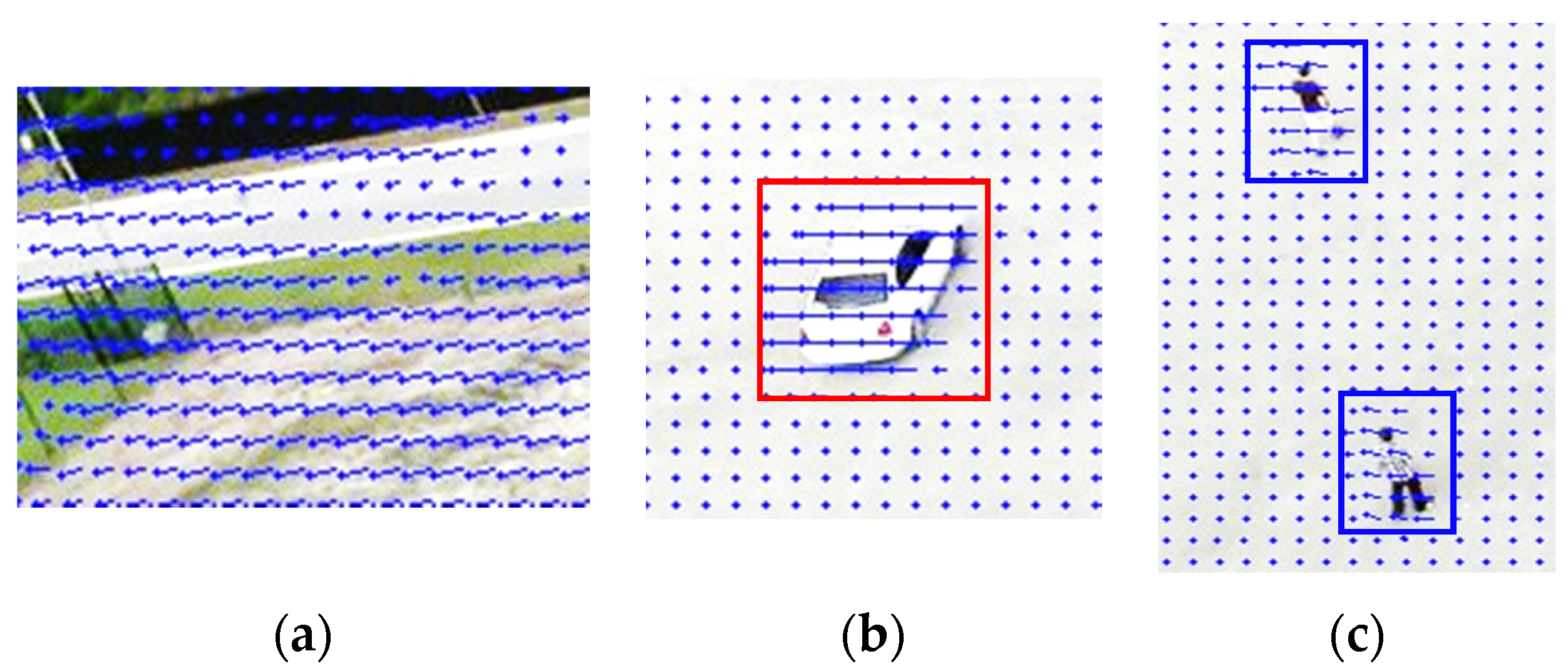
3.1. Result of Motion Vectors

The tested images were unstable due to the movement of the UAV. This caused their motion vectors with regards to static (non-moving) and dynamic (moving) objects to be unsuitable to distinguish. Figure 8 and Figure 9 show the results of the motion vectors without and with image stabilization, respectively. Figure 8a and Figure 9a show the motion vectors in the background. Figure 8b and Figure 9b show the motion vectors in the ROI as a static object car. Figure 8c and Figure 9c show the motion vectors in the ROI as dynamic objects people. Figure 8 shows that the motion vectors of the dynamic and static objects are almost the same with slight difference from the motion vectors in the background. Thus, the result of the motion vectors without image stabilization was incorrect.

Figure 9b shows that the motion vectors in the car (static object) are almost the same as the background. Figure 9c shows that the motion vectors in the people (dynamic objects) are very different from the background. Thus, the results of the motion vectors with image stabilization were very suitable to distinguish between static and dynamic objects.

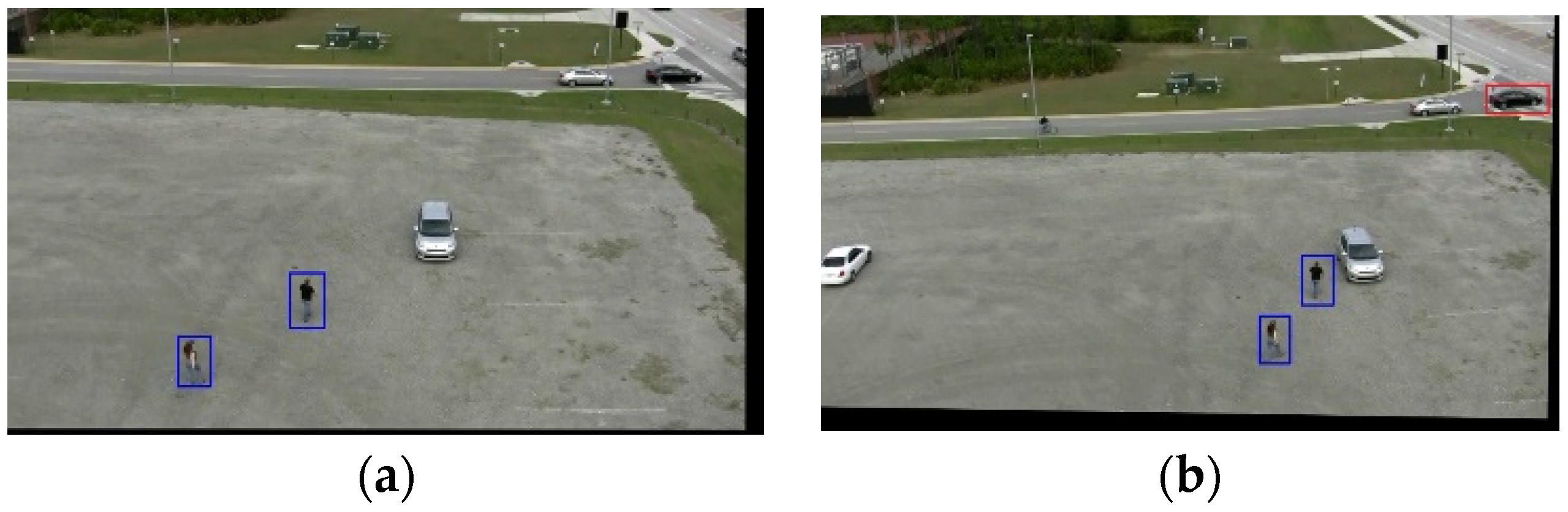
3.2. Result of Moving Objects Detection

Figure 10, Figure 11 and Figure 12 show the results of detection and recognition of moving objects. In some cases, there were false detections on moving objects candidates because motion vectors classified these objects as undesirable and so omitted them. Figure 10 and Figure 11 show the sequence of images obtained from Action1 and Action2, respectively. Sometimes the algorithm did not detect a small object in the image. For example, a small car in Figure 11a was not detected as the foreground. Although the classification result of the motion vector showed the car as a moving object, the final result eliminated the car because the object region was not recognized as the foreground.

Figure 12 shows result of the sequence of images obtained from Action3 which contains five people playing together and making little movements every once in a while. The detection result showed that if there were only slight displacements on an object, it was difficult to distinguish the motion vector. So, the object tended to be detected as a non-moving object.

The results of computation performance are summarized in

Table 1. Computation time performance in frames per second (fps).

Video Name	Average Fps
Action1	49.9
Action2	42.16
Action3	49.2
Average	47.08

in respect of frames per second (fps). The average time cost is about 47.08 fps which is faster than previous methods in [23,24,25,26,27,28].

Table 2. Detection results performance.

Video Name	TP	FP	FN	PR	Recall	F-Measure
Action1	124	7	6	0.95	0.95	0.95
Action2	245	19	23	0.92	0.91	0.91
Action3	184	12	25	0.94	0.88	0.90
Average				0.94	0.91	0.92

shows the performance accuracy in terms of True Positive (TP), False Positive (FP), False Negative (FN), Precision Rate (PR), recall, and f-measure. TP is the detected region that corresponds to the moving object. FP is the detected region that is not related to the moving object. FN is the region associated with the moving object that is not detected. The performance accuracy can be computed as

$$PR=\frac{TP}{TP+FP},$$

(30)

$$\mathrm{Recall}=\frac{TP}{TP+FN},$$

(31)

$$\mathrm{F}\text{-}\mathrm{measure}=2\times \frac{PR\times \mathrm{Recall}}{PR+\mathrm{Recall}}.$$

(32)

Although many articles have tried to solve the same problem (moving object detection using a moving camera), the proposed method has performed well for real-time computation time in a real environment with a complex background. The detection results also showed that the proposed method detected moving objects with high accuracy, although the UAV had some unwanted motion and vibration. The comparison of computation time and accuracy between the results of the proposed method with those methods in [23,24,25,26,28] are reported in

Table 3. Comparison of performance results.

Method	Computation Time (fps)		Accuracy
		PR	Recall	F-Measure
Proposed	47.08	0.94	0.91	0.92
[23]	1	0.7	0.76	0.72
[24]	-	0.66	0.86	0.74
[25]	-	0.94	0.89	0.91
[26]	1.6	-	-	0.73
[28]	5	-	-	0.76

. The proposed method achieved an average precision rate of 0.94 and a recall of 0.91. Action1 had the highest PR and recall compared to other videos because there were only a few objects and their sizes were quite large. Action2 had the lowest PR because there were a lot of objects that were similar to the person and car such as trees, fences, road signs, houses, and bushes. Action3 had the lowest recall due to some small objects in the video with displacement.

The method in [27] did not discuss the accuracy of the detected moving object as well as the computation time performance. It focused on the optical flow to describe the direction of pixel movement. However, this method, i.e., [27], is suitable for application on an image with a homogeneous background. In our case, a moving camera produced several objects in the background that had no correlation with moving objects but had pixel movements. This condition occurs in image sequences that have complex backgrounds such as our datasets. Thus, the method in [27] is not suitable to be applied to our datasets. In addition, we used a simple dense optical flow which is sufficient to calculate the motion vector fields between two consecutive frames and has a fast computation time. Then, we used the classification, which is feasible to distinguish the motion vectors between static and dynamic objects, to determine MD in the background and foreground.

The proposed method can be used for various moving objects, not only for people and cars. In this work, we used people and car objects to test the performance of the method, because these objects are often investigated as moving objects using moving cameras [23,24,25,26,27,28,29]. High frequency jitter, small size objects, and low-quality images make detection of moving objects using UAVs a difficult task. But, using the framework that we propose, we can resolve the problem. Furthermore, a machine learning approach is used to detect and recognize the foreground because it can be applied to almost all processors without GPU. This method is proposed for use on a PC or on-board system. In other words, if the image capture by UAVs can be transmitted to a ground station such as a PC using a wireless camera or transmitted to an additional board such as Raspberry Pi on a UAV, then the image can be processed online and in real time.

Based on information from datasets and previous studies [23,24,25,26,27,28,29], we can conclude that the proposed algorithm will be applicable under the conditions: UAV altitude is less than 500 feet and speed is less than 15 m/s. In addition, based on our experiment results, our algorithm had the best results at a video frame rate of less than 50 fps.

4. Conclusions

A novel method for multiple moving objects detection using UAVs is presented in this paper. The main contribution of the proposed method is to detect and recognize moving objects by using a UAV with moving camera with excellent accuracy and can be used in real-time applications. An image stabilization method was used to handle unwanted motion in aerial images so that a significant difference in motion vectors can be obtained to distinguish between static and dynamic objects. The object detection that was used to determine the region of the moving object candidate had a fast computation time and good accuracy on complex backgrounds. Some false detections can be handled using a motion vector classification, in which the object that has a movement direction similar to the background will be removed as a moving object candidate. Comparing the results on various sequences of aerial images, the proposed method can be a potential real-time application in the real environment.

References

1. Zhou, X.; Yang, C.; Yu, W. Moving object detection by detecting contiguous outliers in the low-rank representation. IEEE Trans. Pattern Anal. Mach. Intell. 2013, 35, 597–610. [Google Scholar] [CrossRef] [PubMed]
2. Kang, B.; Zhu, W.-P. Robust moving object detection using compressed sensing. IET Image Process. 2015, 9, 811–819. [Google Scholar] [CrossRef]
3. Chen, B.-H.; Shi, L.-F.; Ke, X. A robust moving object detection in multi-scenario big data for video surveillance. IEEE Trans. Circuits Syst. Video Technol. 2018, 29, 982–995. [Google Scholar] [CrossRef]
4. Liu, K.; Mattyus, G. Fast Multiclass vehicle detection on aerial images. IEEE Geosci. Remote Sens. Lett. 2015, 12, 1938–1942. [Google Scholar]
5. Wu, Q.; Kang, W.; Zhuang, X. Real-time vehicle detection with foreground-based cascade classifier. IET Image Process. 2016, 10, 289–296. [Google Scholar]
6. Chen, Y.W.; Chen, K.; Yuan, S.Y.; Kuo, S.Y. Moving object counting using a tripwire in H.265/HEVC bitstreams for video surveillance. IEEE Access 2016, 4, 2529–2541. [Google Scholar] [CrossRef]
7. Wang, H.; Oneata, D.; Verbeek, J.; Schmid, C. A Robust and efficient video representation for action recognition. Int. J. Comput. Vis. 2016, 119, 219–238. [Google Scholar] [CrossRef]
8. Lin, Y.; Tong, Y.; Cao, Y.; Zhou, Y.; Wang, S. Visual-attention-based background modeling for detecting infrequently moving objects. IEEE Trans. Circuits Syst. Video Technol. 2017, 27, 1208–1221. [Google Scholar] [CrossRef]
9. Hammoud, R.I.; Sahin, C.S.; Blasch, E.P.; Rhodes, B.J. Multi-source multi-modal activity recognition in aerial video surveillance. In Proceedings of the IEEE Conference on Computer Vision and Pattern Recognition Workshops, Columbus, OH, USA, 23–28 June 2014; pp. 237–244. [Google Scholar]
10. Ibrahim, A.W.N.; Ching, P.W.; Gerald Seet, G.L.; Michael Lau, W.S.; Czajewski, W.; Leahy, K.; Zhou, D.; Vasile, C.I.; Oikonomopoulos, K.; Schwager, M.; et al. Recognizing human-vehicle interactions from aerial video without training. IEEE Robot. Autom. Mag. 2012, 19, 390–405. [Google Scholar]
11. Liang, C.W.; Juang, C.F. Moving object classification using a combination of static appearance features and spatial and temporal entropy values of optical flows. IEEE Trans. Intell. Transp. Syst. 2015, 16, 3453–3464. [Google Scholar] [CrossRef]
12. Nguyen, H.T.; Jung, S.W.; Won, C.S. Order-preserving condensation of moving objects in surveillance videos. IEEE Trans. Intell. Transp. Syst. 2016, 17, 2408–2418. [Google Scholar] [CrossRef]
13. Lee, G.; Mallipeddi, R. A genetic algorithm-based moving object detection for real-time traffic surveillance. Signal. Process. Lett. 2015, 22, 1619–1622. [Google Scholar] [CrossRef]
14. Chen, B.H.; Huang, S.C. An advanced moving object detection algorithm for automatic traffic monitoring in real-world limited bandwidth networks. IEEE Trans. Multimed. 2014, 16, 837–847. [Google Scholar] [CrossRef]
15. Minaeian, S.; Liu, J.; Son, Y.J. Vision-based target detection and localization via a team of cooperative UAV and UGVs. IEEE Trans. Syst. Man Cybern. Syst. 2016, 46, 1005–1016. [Google Scholar] [CrossRef]
16. Gupta, M.; Kumar, S.; Behera, L.; Subramanian, V.K. A novel vision-based tracking algorithm for a human-following mobile robot. IEEE Trans. Syst. Man Cybern. Syst. 2017, 47, 1415–1427. [Google Scholar] [CrossRef]
17. Mukherjee, D.; Wu, Q.M.J.; Nguyen, T.M. Gaussian mixture model with advanced distance measure based on support weights and histogram of gradients for background suppression. IEEE Trans. Ind. Inf. 2014, 10, 1086–1096. [Google Scholar] [CrossRef]
18. Zhang, X.; Zhu, C.; Wang, S.; Liu, Y.; Ye, M. A bayesian approach to camouflaged moving object detection. IEEE Trans. Circuits Syst. Video Technol. 2017, 27, 2001–2013. [Google Scholar] [CrossRef]
19. Xu, Z.; Zhang, Q.; Cao, Z.; Xiao, C. Video background completion using motion-guided pixels assignment optimization. IEEE Trans. Circuits Syst. Video Technol. 2016, 26, 1393–1406. [Google Scholar] [CrossRef]
20. Benedek, C.; Szirányi, T.; Kato, Z.; Zerubia, J. Detection of object motion regions in aerial image pairs with a multilayer markovian model. IEEE Trans. Image Process. 2009, 18, 2303–2315. [Google Scholar] [CrossRef]
21. Wang, Z.; Liao, K.; Xiong, J.; Zhang, Q. Moving object detection based on temporal information. IEEE Signal. Process. Lett. 2014, 21, 1403–1407. [Google Scholar] [CrossRef]
22. Bae, S.-H.; Kim, M. A DCT-based total JND profile for spatiotemporal and foveated masking effects. IEEE Trans. Circuits Syst. Video Technol. 2017, 27, 1196–1207. [Google Scholar] [CrossRef]
23. Yazdi, M.; Bouwmans, T. New trends on moving object detection in video images captured by a moving camera: A survey. Comput. Sci. Rev. 2018, 28, 157–177. [Google Scholar] [CrossRef]
24. Saif, A.F.M.S.; Prabuwono, A.S.; Mahayuddin, Z.R. Moving object detection using dynamic motion modelling from UAV aerial Images. Sci. World J. 2014, 2014, 1–12. [Google Scholar] [CrossRef] [PubMed]
25. Maier, J.; Humenberger, M. Movement detection based on dense optical flow for unmanned aerial vehicles. Int. J. Adv. Robot. Syst. 2013, 10, 146–157. [Google Scholar] [CrossRef]
26. Kalantar, B.; Mansor, S.B.; Halin, A.A.; Shafri, H.Z.M.; Zand, M. Multiple moving object detection from UAV videos using trajectories of matched regional adjacency graphs. IEEE Trans. Geosci. Remote Sens. 2017, 55, 5198–5213. [Google Scholar] [CrossRef]
27. Wu, Y.; He, X.; Nguyen, T.Q. Moving object detection with a freely moving camera via background motion subtraction. IEEE Trans. Circuits Syst. Video Technol. 2017, 27, 236–248. [Google Scholar] [CrossRef]
28. Cai, S.; Huang, Y.; Ye, B.; Xu, C. Dynamic illumination optical flow computing for sensing multiple mobile robots from a drone. IEEE Trans. Syst. Man Cybern. Syst. 2017, 48, 1370–1382. [Google Scholar] [CrossRef]
29. Minaeian, S.; Liu, J.; Son, Y.J. Effective and efficient detection of moving targets from a UAV’s camera. IEEE Trans. Intell. Transp. Syst. 2018, 19, 497–506. [Google Scholar] [CrossRef]
30. Leal-Taixé, L.; Milan, A.; Schindler, K.; Cremers, D.; Reid, I.; Roth, S. Tracking the trackers: An analysis of the state of the art in multiple object tracking. arXiv 2017, arXiv:1704.02781. Available online: https://arxiv.org/abs/1704.02781 (accessed on 10 April 2017).
31. Bay, H.; Ess, A.; Tuytelaars, T.; Van Gool, L. Speeded-Up Robust Features (SURF). Comput. Vis. Image Underst. 2008, 110, 346–359. [Google Scholar] [CrossRef]
32. Shene, T.N.; Sridharan, K.; Sudha, N. Real-time SURF-based video stabilization system for an FPGA-driven mobile robot. IEEE Trans. Ind. Electron. 2016, 63, 5012–5021. [Google Scholar] [CrossRef]
33. Rahmaniar, W.; Wang, W.-J. A novel object detection method based on Fuzzy sets theory and SURF. In Proceedings of the International Conference on System Science and Engineering, Morioka, Japan, 6–8 July 2015; pp. 570–584. [Google Scholar]
34. Kumar, S.; Azartash, H.; Biswas, M.; Nguyen, T. Real-time affine global motion estimation using phase correlation and its application for digital image stabilization. IEEE Trans. Image Process. 2011, 20, 3406–3418. [Google Scholar] [CrossRef] [PubMed]
35. Wang, C.; Kim, J.; Byun, K.; Ni, J.; Ko, S. Robust digital image stabilization using the Kalman filter. IEEE Trans. Consum. Electron. 2009, 55, 6–14. [Google Scholar] [CrossRef]
36. Ryu, Y.G.; Chung, M.J. Robust online digital image stabilization based on point-feature trajectory without accumulative global motion estimation. IEEE Signal. Process. Lett. 2012, 19, 223–226. [Google Scholar] [CrossRef]
37. Viola, P.; Jones, M.J. Robust real-time face detection. Int. J. Comput. Vis. 2004, 57, 137–154. [Google Scholar] [CrossRef]
38. Ludwig, O.; Nunes, U.; Ribeiro, B.; Premebida, C. Improving the generalization capacity of cascade classifiers. IEEE Trans. Cybern. 2013, 43, 2135–2146. [Google Scholar] [CrossRef]
39. Rahmaniar, W.; Wang, W. Real-Time automated segmentation and classification of calcaneal fractures in CT images. Appl. Sci. 2019, 9, 3011. [Google Scholar] [CrossRef] [Green Version]
40. Farneback, G. Two-frame motion estimation based on polynomial expansion. In Proceedings of the Scandinavian Conference on Image Analysis, Halmstad, Sweden, 29 June–2 July 2003; pp. 363–370. [Google Scholar]
41. Cayon, R.J.O. Online Video Stabilization for UAV. Master’s Thesis, Politecnico di Milano, Milan, Italy, 2013. [Google Scholar]
42. Li, J.; Xu, T.; Zhang, K. Real-Time Feature-Based Video Stabilization on FPGA. IEEE Trans. Circuits Syst. Video Technol. 2017, 27, 907–919. [Google Scholar] [CrossRef]
43. Hong, S.; Dorado, A.; Saavedra, G.; Barreiro, J.C.; Martinez-Corral, M. Three-dimensional integral-imaging display from calibrated and depth-hole filtered kinect information. J. Disp. Technol. 2016, 12, 1301–1308. [Google Scholar] [CrossRef]
44. Muja, M.; Lowe, D.G. Fast approximate nearest neighbors with automatic algorithm configuration. In Proceedings of the International Conference on Computer Vision Theory and Applications, Lisboa, Portugal, 5–8 February 2009; pp. 331–340. [Google Scholar]
45. Fischler, M.A.; Bolles, R.C. Random sample consensus: A paradigm for model fitting with applications to image analysis and automated cartography. Commun. ACM 1981, 24, 381–395. [Google Scholar] [CrossRef]
46. Yu, H.; Moulin, P. Regularized Adaboost learning for identification of time-varying content. IEEE Trans. Inf. Forensics Secur. 2014, 9, 1606–1616. [Google Scholar] [CrossRef]
Figure 1. Unmanned aerial vehicles (UAV) movement modeling.
Electronics 08 01373 g001
Figure 2. System overview of the real-time moving object detection and recognition using UAV.
Electronics 08 01373 g002
Figure 3. Haar-like features: (a) Edge, (b) line, (c) center-surround.
Electronics 08 01373 g003
Figure 4. Examples of positive images: (a) Person, (b) car, (c) non-moving object.
Electronics 08 01373 g004
Figure 5. Cascade classifier for object detection and recognition.
Electronics 08 01373 g005
Figure 6. Optical flow estimation: (a) Original image, (b) motion vectors.
Electronics 08 01373 g006
Figure 7. Flowcharts to classify motion vectors and select moving objects.
Electronics 08 01373 g007
Figure 8. Result of motion vectors without image stabilization: (a) Background, (b) car, (c) people.
Electronics 08 01373 g008
Figure 9. Result of motion vectors with image stabilization: (a) Background, (b) car, (c) people.
Electronics 08 01373 g009
Figure 10. The result of moving object detection in Action1: (a) Frame 25, (b) frame 100, (c) frame 210, (d) frame 405.
Electronics 08 01373 g010
Figure 11. The result of moving object detection in Action2: (a) Frame 25, (b) frame 100, (c) frame 170, (d) frame 440.
Electronics 08 01373 g011aElectronics 08 01373 g011b
Figure 12. The result of moving object detection in Action3: (a) Frame 5, (b) frame 60, (c) frame 120, (d) frame 300.
Electronics 08 01373 g012