Airborne LiDAR Point Cloud Filtering by a Multilevel Adaptive Filter Based on Morphological Reconstruction and Thin Plate Spline Interpolation

Abstract

Point cloud filtering is a crucial step in most airborne light detection and ranging (LiDAR) applications. Many filtering algorithms have been proposed, but the filtering effect has some limitations in complex environments. To improve the filtering effect in complex terrain, a multilevel adaptive filter (MAF) combining morphological reconstruction and thin plate spline (TPS) interpolation is proposed. The digital elevation model (DEM) generated in each iteration is used as the marker image for morphological reconstruction to extract ground pixels, and an adaptive residual threshold is achieved by using terrain gradient as a compensation. The benchmark dataset provided by the International Society for Photogrammetry and Remote Sensing (ISPRS) and another LiDAR dataset in northwestern China were used to evaluate the filtering performance of MAF. For the ISPRS benchmark dataset, MAF obtained the lowest average total error (3.72%) and highest average kappa coefficient (87.16%) compared with eight classic filtering algorithms. For the dataset in northwestern China, the DEM generated from the filtering result of MAF obtained higher accuracy than the filtering result of TerraScan. Overall, the MAF achieved promising results without considering the selection of filtering window, which may enhance the robustness and applicability of the algorithm in different environments.

1. Introduction

The development of airborne light detection and ranging (LiDAR) provides a new method for obtaining high-resolution geospatial information. The airborne LiDAR system is mainly composed of global positioning systems (GPSs), laser scanners (LSs), and inertial navigation systems (INSs). The system can acquire three-dimensional (3D) information quickly and accurately by actively emitting laser pulses to the ground. Currently, LiDAR data have been widely used in many fields, such as digital elevation model (DEM) acquisition [1,2], road extraction [3], and forest structural parameter retrieval [4,5,6,7].

In most airborne LiDAR applications, a critical step is point cloud filtering. Point cloud filtering is the process of removing nonground points while retaining terrain points [8,9,10,11]. The filtering result directly affects the quality of the digital elevation model (DEM), which is one of the key factors affecting subsequent processing. Therefore, obtaining ground points quickly, efficiently, and accurately has always been an important issue. In recent years, a large number of filtering algorithms have been proposed. According to the different theoretical backgrounds, these algorithms can be divided into three categories: slope-based [12,13], morphology-based [14,15,16,17], and interpolation-based filtering algorithms [18,19,20,21].

The basic principle of slope-based filtering algorithms is that the slope between ground points is small, while the slope between ground points and nonground points is large. Points with slopes greater than a threshold are classified as nonground points; otherwise, they are classified as ground points. Vosselman [22] noted that the optimal slope threshold can be set according to prior knowledge of the experimental area. Sithole [13] improved the method by adapting a slope threshold that varies according to the actual terrain slope. Susaki [23] achieved a changed terrain threshold by adapting it according to the rough digital terrain model (DTM) of the hierarchical process. Slope-based filtering algorithms have the advantages of simple principles and easy implementation. However, the filtering results of slope-based algorithms depend on the threshold setting. Although some existing algorithms can dynamically adjust the threshold according to the actual terrain, slope-based algorithms cannot achieve good filtering results in steep and complex terrain [24].

The main principle of morphology-based filtering algorithms is that the elevations of nonground points change greatly after the morphological operation. Points with height differences greater than the threshold value are determined as nonground points and filtered. The size of the filtering window has a great influence on the filtering results. A small window cannot remove large buildings, while a large window will result in the loss of details of terrain fluctuation. Zhang et al. [25] proposed a classic progressive morphological filtering method to solve this problem. In this method, the window grows from small to large, and different windows correspond to different thresholds. Hui et al. [26] combined a morphological operation and kriging interpolation to calculate the topographic relief of local regions at each level and optimized the filtering criteria. Li et al. [24] proposed an improved top-hat filter with a sloped brim to enhance the filtering performance for protruding terrain. Overall, morphology-based filtering algorithms are simple in principle and efficient to implement, but the filtering results are sensitive to the size of the filtering window. Although different algorithms have been developed, the morphology-based filtering algorithms are easy to misclassify points in protruding terrains [26]. The robustness of morphology-based algorithms in areas with large terrain fluctuations still needs to be improved.

The interpolation-based filtering algorithms usually use a certain interpolation method to establish a rough terrain surface, and points are classified according to the residuals from the surface. Axelsson [27] proposed a progressive triangulated irregular network (TIN) densification filtering algorithm. In this algorithm, a sparse TIN was created based on a set of ground seed points. In each iteration, points with an iteration angle and a distance less than a threshold were added, and a new TIN was created. The iterative process continues until no more points can be added. Mongus and Žalik [28] proposed a parameter-free multilevel interpolation-based filtering method. The terrain surface was obtained by interpolating the control points with thin plate spline (TPS), and the points were filtered stepwise until the bottom level. Chen et al. [29] improved the TPS interpolation method in seed points selection and filtering judgment and improved the overall accuracy. Hu et al. [30] calculated the bending energy as a byproduct of TPS interpolation and achieved an adaptive filtering threshold by using it as a threshold compensation. However, interpolation-based algorithms are usually time consuming and have difficulties in filtering areas with break lines, steep, and highly variable terrain [15].

Although many filtering algorithms have been developed and successfully applied, the filtering effect has some limitations in complex environments. Researchers have tried to combine different algorithms to improve the filtering accuracy. Bigdeli et al. [19] integrated the filtering results of slope-based and morphological-based algorithms and achieved promising results for dense forests. The segmented point clouds can provide more semantic information, which is helpful for the subsequent filtering judgment. Lin and Zhang [31] used a region-growing method to divide point clouds into different sections; then, they selected ground seed points and established the initial TIN, and obtained the final ground point cloud using the progressive TIN densification algorithm. To protect the terrain details in protruding areas, Zhang and Lin [1] embedded the smoothness-constrained segmentation method in the progressive TIN densification method. The results showed that the method can effectively reduce type I error.

The combination of filtering algorithms based on different principles may help overcome the limitations of a single algorithm and improve the filtering accuracy. To enhance the filtering ability in complex environments and preserve the terrain details of protruding areas, this paper proposes the multilevel adaptive filter (MAF) by combining morphological reconstruction and multilayer TPS interpolation. The MAF achieved an adaptive residual threshold without the selection of a filtering window and optimized the process of ground seeds selection in the iteration. Filtering results show that the MAF improves the filtering effect of complex terrains, which may contribute to point cloud filtering for forest structural parameter retrieval, road extraction, and other applications.

The main contributions of proposed algorithm are:

• Ground pixels can be extracted by using rough DEMs for morphological reconstruction, which avoid the selection of the filtering window and enhance the robustness of the algorithm.
• The filtering effect of complex terrain can be improved, and more terrain details can be preserved by adjusting the residual threshold according to the terrain gradient.
• In the process of ground seeds updating, nonground points can be detected and removed to mitigate the influence of misclassification in previous iterations.

2. Materials and Methods

2.1. Experimental Data

The benchmark dataset provided by the International Society for Photogrammetry and Remote Sensing (ISPRS) was used to evaluate the performance of the MAF. The test areas are located in the Vaihingen/Enz test field and Stuttgart city, covering a varied landscape. The benchmark dataset was collected by an Optech ALTM scanner, including 15 samples: nine in urban areas and six in rural areas. For urban areas (from samp11 to samp42), the average point spacing is 1.0–1.5 m, and for rural areas (from samp51 to samp71), the average point spacing is 2.0–3.5 m. For each sample, the benchmark data were obtained by semiautomatic filtering and manual editing.

Another LiDAR dataset located in the Heihe River Basin in northwestern China was used to evaluate the performance of MAF in dense forests. The study area is a water source protection area called Dayekou, located between 97°24’–102°10’E and 37°41’–42°42’N, and it is a core experimental site in the Watershed Allied Telemetry Experimental Research (WATER) project [32]. The study area covers an area of approximately 130 km² with an altitude of 2500 to 3300 meters, and the main tree species is Picea crassifolia. Airborne LiDAR data was acquired by a RIEGL LiteMapper-5600 airborne laser scanning system on 23 June 2008. The average point density is approximately 3.43 points/m². The study site contains 35 square forest plots, including 16 plots that make up a superplot and 19 plots along a linear transect (line plot) [5]. The size of the subplots from the superplot is 25 m, and the center and corner locations of each subplot were positioned by a differential global positioning system (DGPS) station. The size of the subplots from the line plot is 20 m, the distance from the center of the adjacent subplot is 50 m, and the center location of each subplot was positioned by a DGPS station.

2.2. Filtering Procedure

The interpolation-based filtering algorithms classify point clouds according to their residuals to the interpolated surface. However, the threshold value has a significant influence on the filtering result. The influence of complex terrain should be considered when filtering point clouds, because a fixed residual threshold may not obtain satisfactory filtering results when the terrain fluctuates greatly. Compared with flat terrain, there should be a greater residual threshold on steep terrain. In order to improve the filtering accuracy in complex environments, this paper proposes MAF by combining morphological reconstruction and three-level TPS interpolation. At each level, a digital surface model (DSM) and a rough DEM are generated by TPS interpolation. To suppress the omission error caused by terrain fluctuations, an adaptive filter is achieved by compensating the residual threshold according to the terrain gradient. Ground pixels are extracted by using the rough DEM as the marker image for morphological reconstruction, and the height threshold is compensated at only the ground pixels to avoid commission error. Points with residuals less than the threshold are added to the ground points, and the surface is updated by new ground seeds. The iteration continues until no new ground points are found.

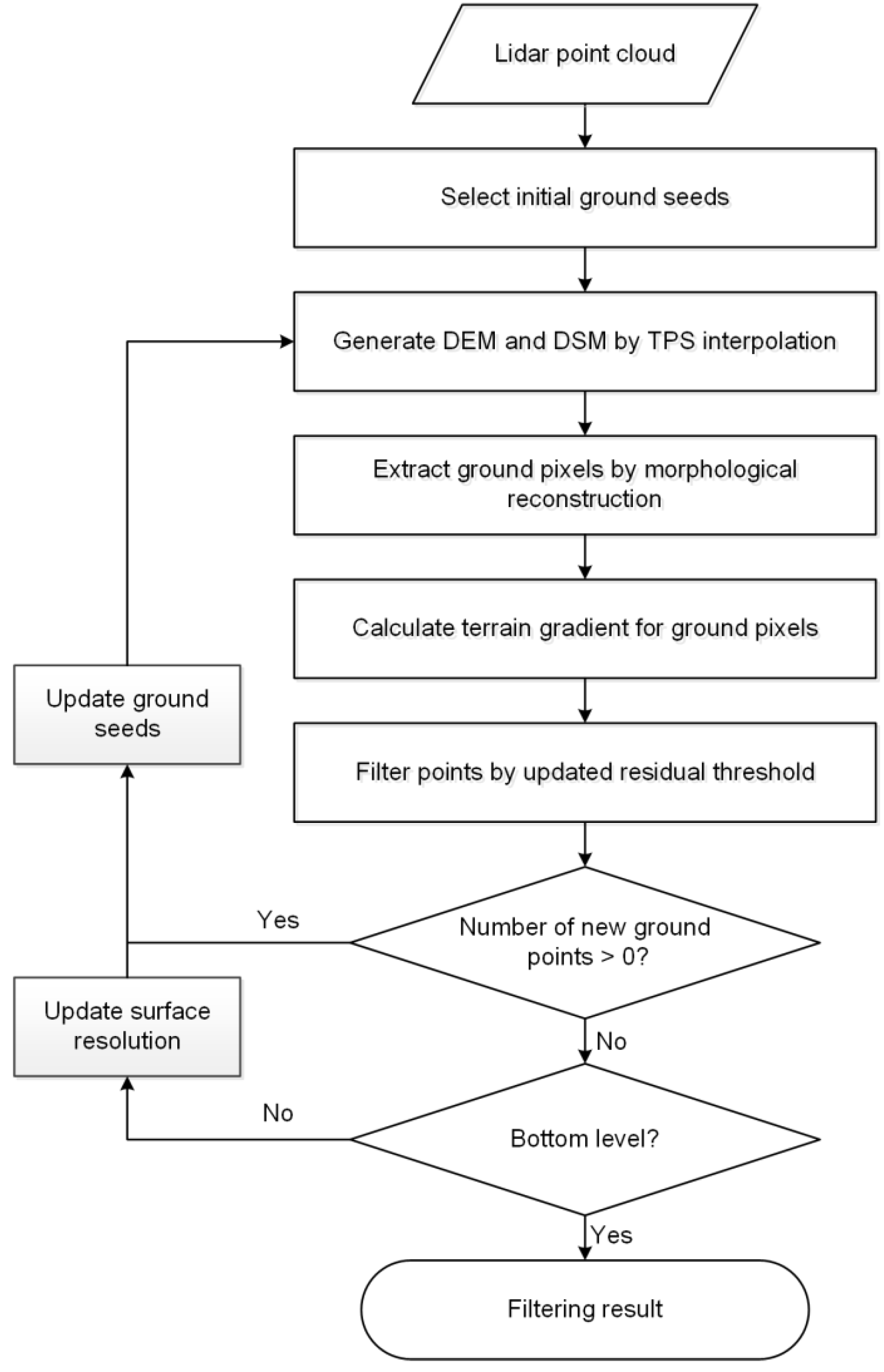
The MAF procedure is as follows, as shown in Figure 1.

(1) Select initial ground seeds. According to the extended local minimum method, find seed points in the window as initial ground seeds;

(2) At the beginning of each level, generate a DSM of the current resolution according to the TPS interpolation. In each iteration, generate a DEM of the current resolution according to the TPS interpolation by ground seeds;

(3) Use the DSM as a mask and the DEM as a marker for morphological reconstruction. Ground pixels are extracted according to the reconstruction results, and the residual threshold t at the ground pixels is updated by the terrain gradient;

(4) Calculate the point cloud distance residuals to nine surrounding pixels. If there are at least four residuals less than the residual threshold t, the point is classified as a ground point [29];

(5) Update the ground seeds, and the grid size is equal to surface resolution;

(6) Repeat steps 2–5 until no ground points are found;

(7) Halve the surface resolution and update T₁ and T₂, and repeat steps 2–6 until the bottom level.

2.2.1. Selection of Initial Ground Seed Points

Usually, the lowest point in a window is considered the initial ground seed. This method is simple and convenient. However, due to multipath reflex and LiDAR system errors, low outliers may be regarded as seed points, which results in a reduction in filtering accuracy and consequently affects the final DEM accuracy. Therefore, this paper applies the extended local minimum method proposed by Chen et al. [15] to find the initial ground seeds. Multiple low points within the window are selected. If the height difference between the lowest point and the second lowest point is less than a given threshold (the value used in this paper is 1 m), the lowest point is considered a seed point. If the height difference is greater than the threshold, the lowest point is considered a low outlier, and the height difference between the second lowest point and the third lowest point is calculated and compared with the threshold. This process continues until the seed point that meets the criteria is found. The size of the search window for the initial seed points should be large enough to avoid the influence of buildings. The value used in this paper is 30 m for most of the samples, except for samp22 and samp42 (35 m).

2.2.2. TPS Interpolation

The interpolation-based algorithms filter point clouds based on the distance residual of points from the interpolated surface. If the distance residual is less than a given threshold, the point is classified as a ground point. Therefore, a good interpolation method needs to accurately approximate the terrain and thus improve the filtering accuracy. The TPS interpolation is considered an accurate interpolation method and has been widely used for point cloud filtering [28,29,30].

TPS interpolation produces a smooth surface that passes through all control points and minimizes bending energy [28,33]. The surface can be expressed as:

$$\mathrm{f}\left(x,y\right)=a_0+a_{1}x+a_{2}y+{{\displaystyle \sum }}_{i=1}^N{w}_{i}q\left(r_i\right)$$

(1)

where $a_0$, $a_1$, and $a_2$ are polynomial coefficients, $N$ is the number of control points used for TPS calculation, and $r_i$ is the distance from the interpolation point to the ith point. $w_i$ is the weight of the control point, and satisfies:

$$\{\begin{array}{c}{\displaystyle \sum }_{i=1}^N{w}_i=0\\ {\displaystyle \sum }_{i=1}^N{w}_i{x}_i=0\\ {\displaystyle \sum }_{i=1}^N{w}_i{y}_i=0\end{array},$$

(2)

q(r) is a radial basis function that can be expressed as:

$$\mathrm{q}\left(\mathrm{r}\right)=r^2\ln \left(r^2\right),$$

(3)

Based on Equations (1) and (2), the matrix equation of TPS can be expressed as:

$$\left[\begin{array}{cc}Q& P\\ P^T& 0\end{array}\right]\left[\begin{array}{c}w\\ a\end{array}\right]=\left[\begin{array}{c}f\\ 0\end{array}\right],$$

(4)

where $Q$ is the $N\times N$ matrix defined by q (r_ij), $a$ is the polynomial coefficient, and $f$ is the measured value.

To improve computational efficiency, this paper uses a local TPS approach [34,35]. For a point to be estimated, only its neighbors are used for interpolation. Neighboring points can be selected by a fixed radius or a fixed number. In this paper, a fixed number is used, and the number of neighboring points is 12, which is consistent with Chen et al. [29].

2.2.3. Morphological Reconstruction

To avoid excessive commission error, the residual threshold is compensated only at ground pixels. Ground pixels are extracted by morphological reconstruction. The morphological reconstruction is accomplished by using two images, a marker image and a mask image, for geodesic dilation [36]. The dilation is repeated continuously, and the mask image is used to limit the dilation propagation [36].

$${\delta }_G^{\left(n\right)}\left(F\right)=\left[\left[\left[\left(F\oplus B\right)\Delta G\right]\oplus B\right)\Delta G\right]\dots \oplus B{)}^{\left(n\right)}\oplus B],$$

(5)

where F is the marker image, G is the mask image, n is the number of stepwise iterations, ⊕ is the dilation operator, and Δ is the pointwise minimum operation [19].

Bigdeli et al. [19] extracted nonground pixels through morphological reconstruction. DSM was used as the mask image, and DSM with a subtracted h-shift value was used as the marker image. Bigdeli et al. [19] iterated a series of h values and integrated their results as nonground pixel extraction results. However, the determination of h usually needs prior knowledge, and the value directly affects the extraction result. If the value is small, nonground pixels cannot be extracted. If the value is large, some ground pixels will be misclassified as nonground pixels. Since the difference between DEM and DSM is a height element associated with nonground points, this study subtracts the rough DEM of each iteration from the DSM as the h-shift. Therefore, the DSM is used as the mask image, and the DSM with the subtracted h-shift (e.g., the DEM) is used as the marker image.

At each level, a DSM and a DEM are generated based on the TPS interpolation. In each iteration, the mask image is subtracted from the reconstructed result to produce a normalized DSM (nDSM). Connected areas in the nDSM image are marked, and parcels with an average height less than T₁ are considered ground pixels.

ground_mask = {Z_i < T₁}, i = {1, 2, … n},

(6)

where Zi is the mean elevation of the detected parcel, T₁ is the elevation threshold, n is the number of labeled parcels, and ground_mask is a binary indicator of ground pixels.

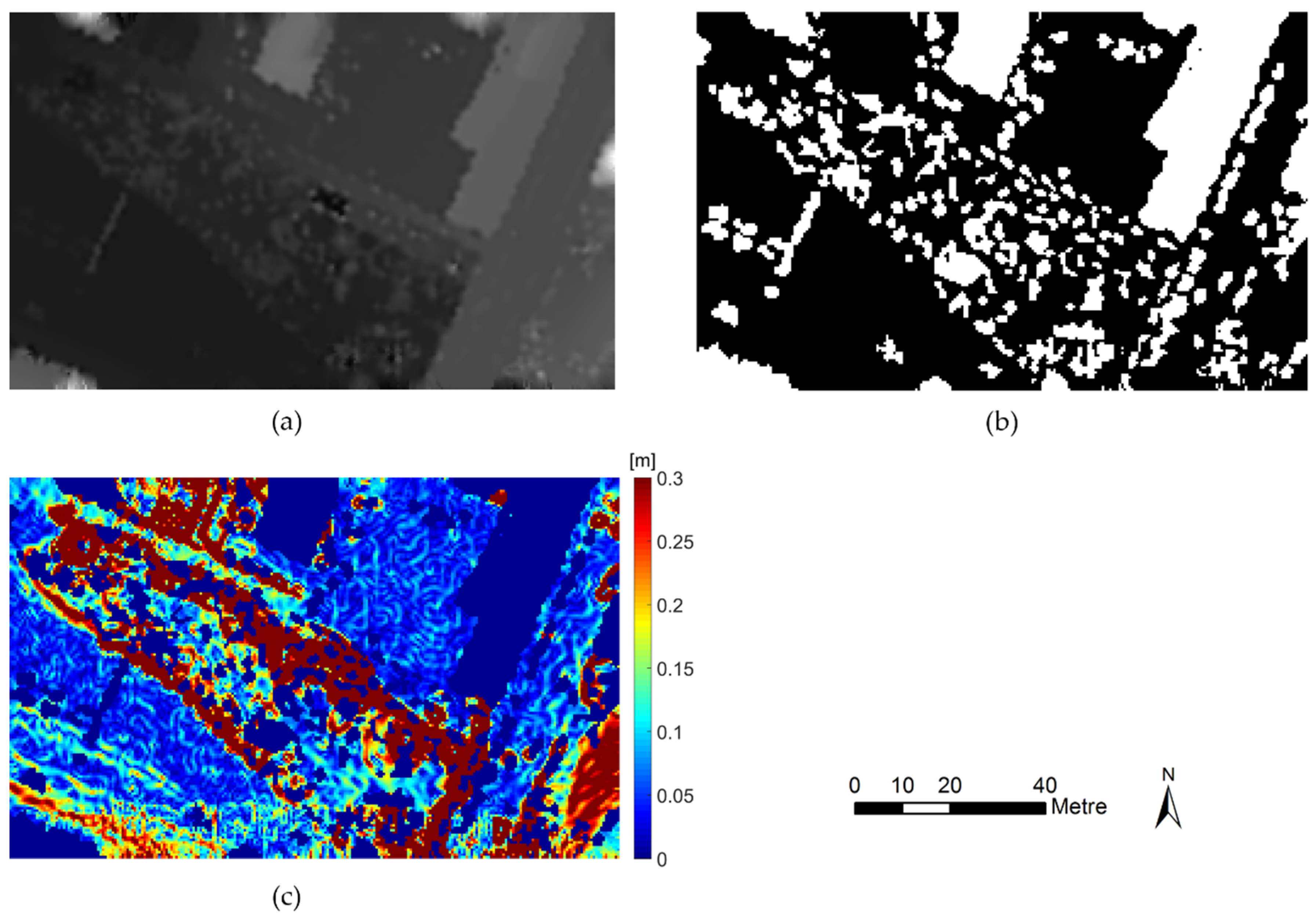
The vertical and horizontal components of the numerical gradient of the DEM are calculated, which are the differences in the corresponding directions. The terrain gradient is calculated according to the two components, and the gradient is used for compensating the residual threshold with an upper bound of 0.3 m, as shown in Figure 2. The gradient compensation (Figure 2c) is achieved based on the terrain gradient and the ground_mask (Figure 2b) as a binary indicator of ground pixels that control where the threshold compensation is performed to avoid commission error. The residual threshold t is determined as:

t = T₂ + gradient_gain * ground_mask,

(7)

where T₂ is a user-defined parameter, and gradient_gain is the threshold compensation according to the terrain gradient.

2.2.4. Update Ground Seeds

In the iteration of interpolation-based filtering algorithms, the surfaces are interpolated by the ground seeds. The ground seeds are updated based on previous filtering results, and the lowest ground point in each grid cell is usually considered as the ground seed [29]. However, nonground points might be selected as ground seeds as a result of a misclassification of the previous iteration, and it would in turn induce more commission errors. To avoid that, this study updates ground seed by considering its relationship with neighboring seeds in a 3 × 3 window. Firstly, ground seeds are selected by the local minimum method. In the first two levels of filtering, seeds with elevation higher than a threshold T₃ are considered as nonground points and removed. T₃ is defined as:

T₃ = meanH + 3 × stdH,

(8)

where meanH is the mean elevation of neighbor seeds within the window, and stdH is the standard deviation of the neighbor seeds elevation.

2.3. Parameter Settings

For all datasets, one set of parameters is used in this paper. The initial resolution of DEM and DSM is 2 m. When the iterations begin, a limited number of seed points are used for interpolation. To avoid introducing too many nonground points, the initial values of T₁ and T₂ are 0.5 m and 0.2 m, respectively. With the change in scale, the surface becomes more accurate, so T₁ and T₂ increase by −0.1 m and 0.1 m at each level, respectively.

2.4. Accuracy Evaluation

In this paper, the MAF filtering result is evaluated by four precision indices, including the omission error, commission error, total error [37], and the kappa coefficient [38]. The omission error, also known as a type I error, is the percentage of ground points misclassified as nonground points, while the commission error, referred to as a type II error, is the percentage of nonground points accepted as ground points. The total error is the percentage of misclassified points in all points. In addition, the kappa coefficient is considered to be a more robust measurement than a simple percentage, and has been widely used in previous work [26,30,39]. Compared with the random classification, the kappa coefficient is an alternative measure of the overall classification accuracy, which subtracts the influence of accidental consistency and quantifies the effect of the specific classification [29].

3. Results and Discussion

Table 1. Filtering accuracy for all the ISPRS samples.

Sample	Type I (%)	Type II (%)	Total (%)	Kappa (%)
samp11	8.05	13.09	10.20	79.09
samp12	1.90	4.11	2.97	94.05
samp21	0.18	5.46	1.35	96.02
samp22	2.24	7.28	3.82	91.05
samp23	5.19	4.85	5.03	89.92
samp24	3.39	10.06	5.22	86.86
samp31	0.44	4.11	2.13	95.69
samp41	9.26	3.55	6.40	87.19
samp42	0.67	0.65	0.66	98.42
samp51	0.29	6.78	1.71	94.89
samp52	2.55	10.58	3.39	82.82
samp53	6.37	11.66	6.58	49.12
samp54	3.41	2.51	2.93	94.11
samp61	2.02	4.23	2.10	74.82
samp71	0.80	5.59	1.34	93.33
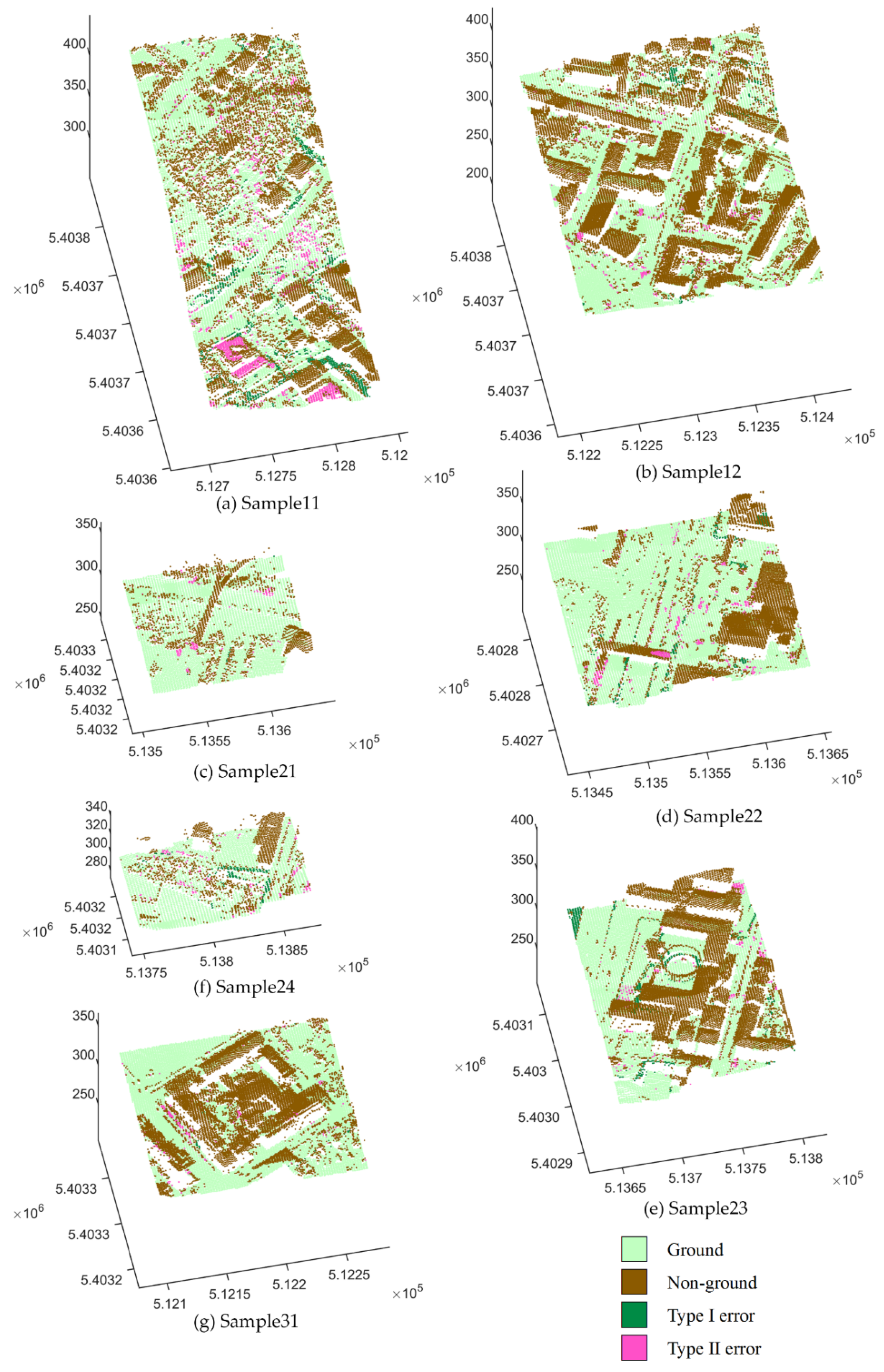
Average	3.12	6.30	3.72	87.16

and Figure 3 show the filtering accuracy and error distribution of the MAF for the ISPRS benchmark dataset, respectively. For samples located in flat regions, the MAF achieved high filtering accuracy. Eight samples, including samp12, 21, 22, 31, 42, 51, 54, 71, obtained a kappa coefficient greater than 90%, and the total errors of these samples were less than 4%. For samples located in regions with complex terrain, the filtering results had relatively high errors. The MAF achieved a total error greater than 10% at samp11 with varied terrain and buildings and low vegetation on steep slopes. The results are consistent with the conclusion that filtering algorithms usually perform well in fairly flat terrain, but the performance tends to be less stable as the slope of the terrain increases [37]. Buildings with different sizes and complex shapes in samp12, 23, 31 and 41 were effectively removed. The type II error of samp53 exceeded 10% due to the presence of terrain discontinuities. Some low object points in samp23 and samp54 were not successfully removed, as there were no significant height differences between objects and ground points. The MAF obtained higher type II errors than type I errors at almost all the samples as a result of nonground points are generally less than the ground points. The MAF achieved high type II errors in samp61 and samp71 because very few nonground points are located in the two samples, while the numbers of type I errors and total errors of the two samples were small. Overall, the proposed filtering method can achieve promising and reliable results for diverse landscapes.

To objectively evaluate the MAF filtering effect, the MAF filtering results were compared with the eight classic algorithms of the ISPRS test [13,27,37,40,41,42,43,44,45]. The comparison results are shown in

Table 2. Comparison of MAF total errors and the eight classic algorithms for all the ISPRS samples (the bold value is the smallest value in each line and indicates that the corresponding method had the best performance for the study site).

Sample	Eight Classic Algorithms (%)	MAF (%)
samp11		10.20
samp12		2.97
samp21		1.35
samp22	3.63 (Axelsson (2000))	3.82
samp23	4.00 (Axelsson (2000))	5.03
samp24	4.42 (Axelsson (2000))	5.22
samp31	1.80 (Pfeifer (1999))	2.13
samp41		6.40
samp42		0.66
samp51		1.71
samp52	3.07 (Axelsson (2000))	3.39
samp53		6.58
samp54		2.93
samp61	2.08 (Axelsson (2000))	2.10
samp71		1.34
Average		3.72

and

Table 3. Comparison of MAF kappa coefficients and the eight classic algorithms for all the ISPRS samples (the bold value is the largest value in each line, and indicates that the corresponding method had the best performance for the study site).

Sample	Eight Classical Algorithms (%)	MAF (%)
samp11		79.09
samp12		94.05
samp21		96.02
samp22	91.33 (Axelsson (2000))	91.05
samp23	91.97 (Axelsson (2000))	89.92
samp24	88.50 (Axelsson (2000))	86.86
samp31	96.37 (Pfeifer (1999))	95.69
samp41		87.19
samp42		98.42
samp51		94.89
samp52	83.63 (Axelsson (2000))	82.82
samp53		49.12
samp54		94.11
samp61		74.82
samp71		93.33
Average		87.16

. The accuracy evaluation indicators are the average kappa coefficients and average total errors of the 15 samples. The MAF obtained the lowest total errors in nine of 15 samples (including samp11, 12, 21, 41, 42, 51, 53, 54, and 71) and the highest kappa coefficients in 10 of 15 samples (including samp11, 12, 21, 41, 42, 51, 53, 54, 61, and 71). The total errors and kappa coefficients of the remaining samples were also close to the optimal results. The MAF outperformed the eight classic algorithms in almost all the samples in rural areas, which indicated that the MAF can preserve more terrain details in rural areas. The algorithm proposed by Axelsson [27] obtained better results than the MAF at some urban samples, which as a result of the MAF misclassified some points that were located in regions where the height differences were not obvious. Overall, the MAF had the best performance, with an average total error of 3.72% and an average kappa coefficient of 87.16%.

In recent years, many filtering algorithms have been proposed and successfully applied. Therefore, in addition to the above eight classic filtering algorithms, four recently developed methods were used to compare with the MAF. Chen et al. [29] proposed a multilayer filtering algorithm based on TPS interpolation. Hu et al. [30] used the bending energy generated in TPS interpolation as a threshold compensation to achieve an adaptive threshold. Hui et al. [26] proposed an algorithm based on morphological open operation and multilayer kriging interpolation to preserve the features of raised terrain. Li et al. 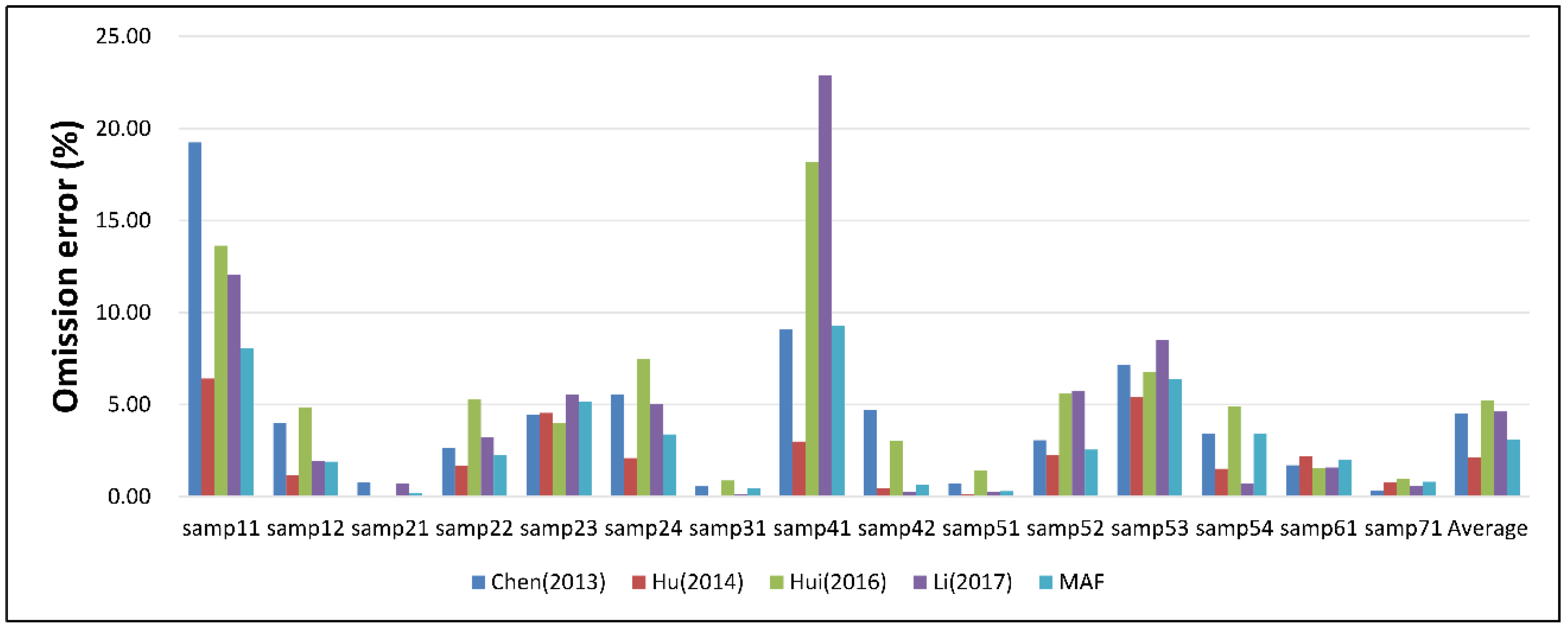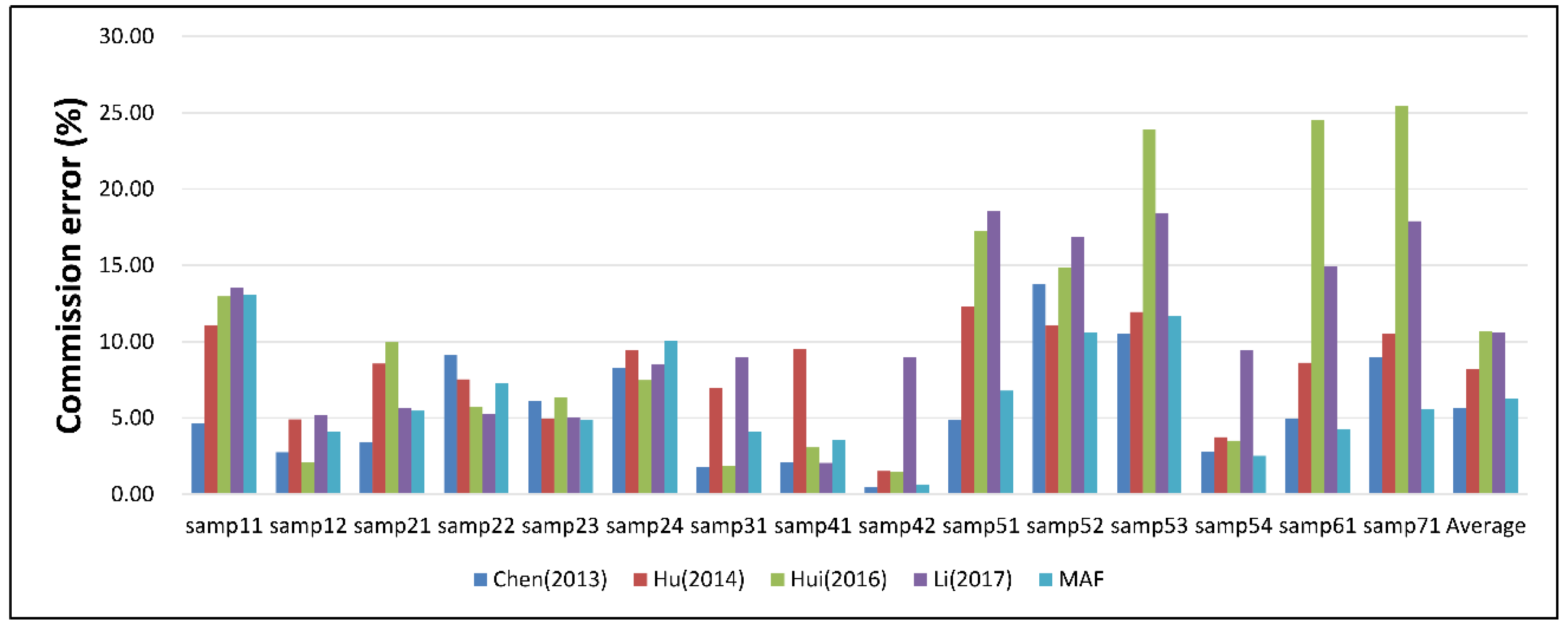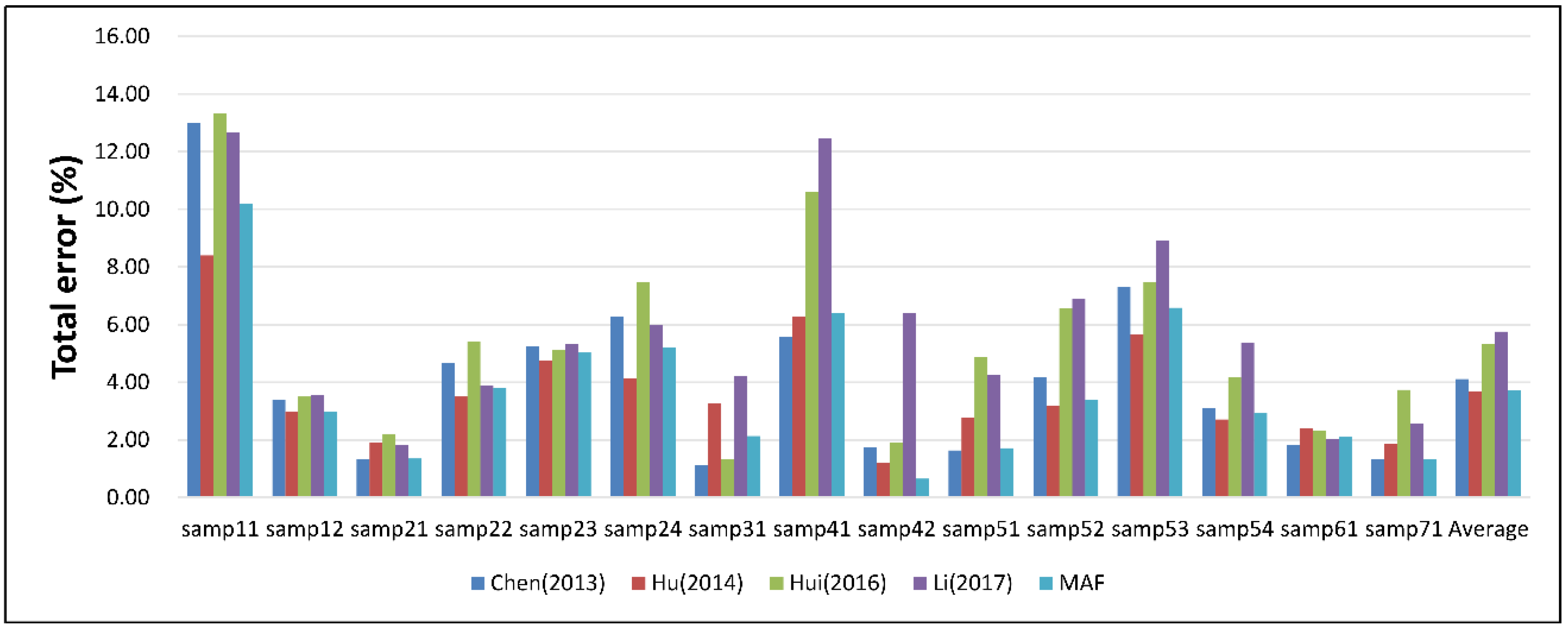[46] proposed an algorithm based on geodesic transformations. The MAF omission error, commission error, and total error were compared with these algorithms, as shown in Figure 4, Figure 5 and Figure 6. The MAF obtained the second lowest average total error for all samples, and it outperformed other algorithms in rural areas. Chen (2013) used different initial thresholds for different samples, while the MAF used identical parameters for all samples, which may enhance the robustness of the algorithm for diverse environments. Hu (2014) used bending energy as the threshold compensation, which induced more commission errors while reducing the omission errors. The commission errors tended to increase as the omission errors decreased. Compared with Chen (2013) and Hu (2014), the MAF compensated for the residual threshold only at ground pixels, which suppressed the omission error without significantly increasing the commission error. Hui (2016) combined the progressive morphological operation and multilayer interpolation, but the algorithm cannot handle the issue caused by the selection of structural elements. Li (2017) implemented geodesic transformations to avoided the influence of the filtering window. However, Li (2017) tends to achieve high commission errors at samp42 and other samples in rural areas.

The MAF took advantage of morphological reconstruction and multilayer TPS interpolation, and improved the adaptivity for different environments and the filtering effect, especially in rural areas. Compared with other algorithms, the MAF considered the process of ground seeds updating during the iteration, and prevented the commission error caused by nonground points being selected as ground seeds.

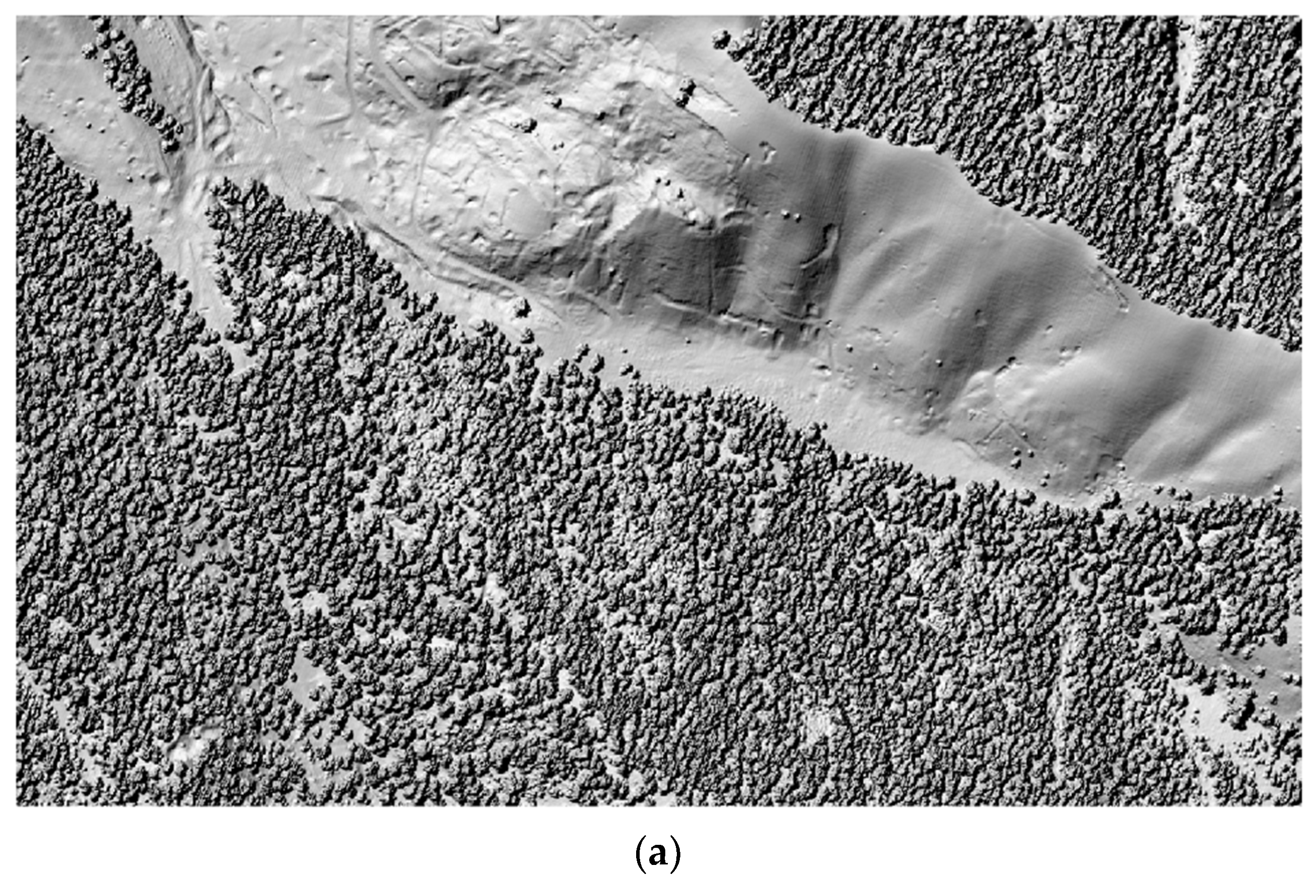
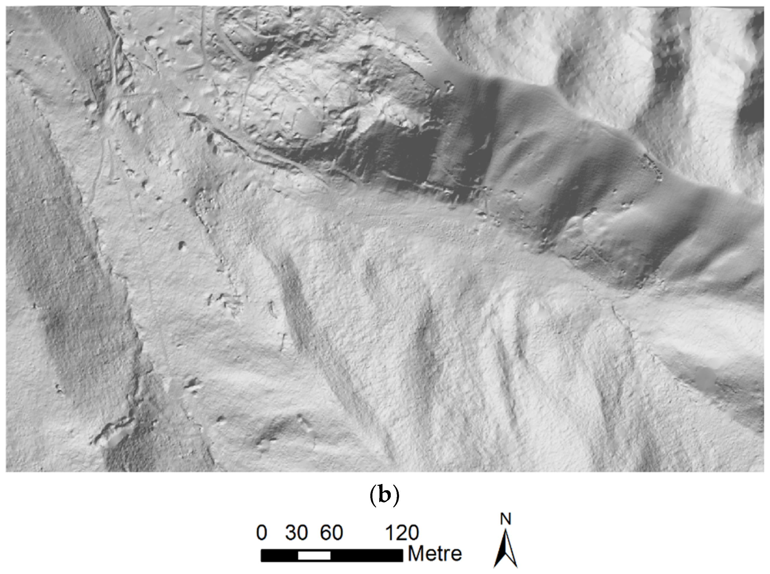
Figure 7 shows the filtering effect of the MAF of the Dayokou data. The landscape of the area is complex, including dense forests, terrain with fluctuations, and steep slopes. The results showed that dense forests were filtered, and low vegetables on slopes and trees along the cliff were effectively removed, while the terrain details were preserved well. The filtering results of TerraScan were used to compare against the MAF. The ground points of the two methods were used to generate DEMs through four interpolation methods, including inverse distance weight (IDW), natural neighbor (NN), ordinary kriging (OK), and universal kriging (UK). The position coordinates of the 35 subsamples measured by DGPS were used as control points to test the DEM accuracy, and the root mean square error (RMSE) of the elevation between control points and the generated DEM is shown in

Table 4. Elevation root mean square error (RMSE) comparison of Dayekou data filtered by MAF and TerraScan. IDW: inverse distance weight, NN: nearest neighbor, OK: ordinary kriging, UK: universal kriging.

Filtering Method	IDW (m)	NN (m)	OK (m)	UK (m)
MAF	0.9249	0.9185	0.9212	0.9210
TerraScan	0.9408	0.9381	0.9402	0.9344

. For all four interpolation methods, the accuracy of the DEM generated from filtering results of the MAF was better than that of TerraScan, indicating that the MAF can obtain promising filtering results for dense forest.

It can be found that the MAF performed well in rural areas, but it misclassified some points around buildings and small objects, where the height differences were not significant. Object edges usually have large gradients as there are height jumps. Nonground points on the object edges might be misclassified as ground points as a result of residual compensation. Besides, the filtering results of interpolation-based algorithms are affected by the results of the previous iteration. If nonground points are selected as ground seeds, adjacent nonground points will be accepted as ground points, which may result in a large commission error area. This study updated ground seeds by considering its relationship with neighbors to mitigate the impact of misclassification in previous iterations. Subsequent research should improve the ground seeds selection rules and consider the error transmission in the iterative process to avoid commission error.

4. Conclusions

In this paper, a filtering algorithm combining morphological reconstruction and multilevel TPS interpolation was proposed. An adaptive filter was achieved by adjusting the residual threshold at ground pixels according to the terrain gradient. To extract ground pixels, rough DEMs generated during the iteration were used as marker images for morphological reconstruction instead of a series of h-shift values, which need to be determined by prior knowledge. The benchmark dataset provided by ISPRS and another dense forest point cloud in northwestern China were used to test the filtering performance. Compared with classic filtering algorithms, the MAF obtained promising and comparable results in urban areas, and it outperformed these algorithms at most samples in rural areas. The MAF avoided the selection of the filtering window in most classic morphology-based filtering algorithms and improved the robustness and filtering performance for complex terrain. The proposed method can be applied for 3D city visualization and objects extraction in urban areas. As the MAF achieved better performance in rural areas, it is also suitable for forest inventory applications. Filtering results of the MAF can be used to generate high-precision DEM, which is helpful for individual tree delineation, forest dynamics monitoring, and the retrieval of key forest parameters. However, some points without significant height differences were misclassified. Therefore, the filtering effect around small objects, discontinuities, and buildings with complex shapes should be improved in further study. The initial ground seeds have a significant influence on the filtering results. Further study should optimize the selection rules of initial seeds to enhance the robustness of the method. Moreover, misclassification during the iterations should be taken into account to mitigate its impact on subsequent iterations.