Applying the Haar-cascade Algorithm for Detecting Safety Equipment in Safety Management Systems for Multiple Working Environments

Abstract

There are many ways to maintain the safety of workers on a working site, such as using a human supervisor, computer supervisor, and smoke–flame detecting system. In order to create a safety warning system for the working site, the machine-learning algorithm—Haar-cascade classifier—was used to build four different classes for safety equipment recognition. Then a proposed algorithm was applied to calculate a score to determine the dangerousness of the current working environment based on the safety equipment and working environment. With this data, the system decides whether it is necessary to give a warning signal. For checking the efficiency of this project, three different situations were installed with this system. Generally, with the promising outcome, this application can be used in maintaining, supervising, and controlling the safety of a worker.

1. Introduction

Since the introduction of Industry 4.0 (I4) in 2011 at the Hannover Fair in Germany, automation and machine learning (ML) have piqued the interest of researchers to apply them to industry, agriculture, and other services. This field forms an important part of modern business and research. ML can improve computing performance in processes pertaining to a single factory or system, a chain of factories, or multi-systems used in any organization. I4 will benefit human society when it synergizes artificial intelligence (AI) with automation in production. In this century, four billion people are connected through the Internet, and there exist 50 trillion gigabyte of data and 25 million tablet and PC applications. All of them have been developed based on I4’s revolution. In addition, the effect of I4 spreads to each field of human life such as agriculture, industry, medical, and education. In Germany, 75% of the factories are smart factories that use AI to control manufacturing systems. To compete with this development trend, the Korean Government has requested many corporations and factories to develop a smart system. With this urgency, collaboration among scientific fields such as computer science, chemistry, and physics is mandatory to cope with current trends. The applications of ML are various, e.g., object recognition, face detection, spoken language understanding, customer segmentation, and weather prediction. As hazardous chemicals need to be handled in chemical engineering, an intelligent system that can control and maintain the safety level of a working environment is urgently demanded. Therefore, in this research, a safety system is introduced that can remind workers to wear personal protective equipment when they are working in a dangerous environment. This system is the combination of some preprocessing algorithms, the ML Haar-cascade algorithm, and system control. The Haar cascade is an ML object detection algorithm used to identify objects in an image or video and is based on the concept of features proposed by Paul Viola and Michael Jones in their paper [1]. Complete learning is always based on typical observations or data, i.e., programming by examples. This system includes several steps such as training classifiers and applying classifiers. The training-classifier step comprises processes such as obtaining data (images) from video, applying preprocessed images, categorizing images to several groups, and training these images using the cascade algorithm. Moreover, the applying-classifier steps include collecting images from video, detecting safety objects, calculating a safety score, and providing feedback based on the safety score. With this research, industrial companies will be able to detect and control a working environment’s safety automatically with the assistance of computers. And the Safety Management System (SMS) is one of the cornerstones of the safety regulatory framework that helps to ensure a high level of safety of a company. This system from this paper could be an intelligence SMS part of the firms’ AI in the I4.0 century.

There are a lot of other equipment used in a normal environment, such masks, safety cloth for the lab, and safety cloth for workers in different working environments. In this study, our system was set only for four classes (human, safety helmet, hooks, and gloves) because the others require a very large dataset. For example, there are many types of masks and cloth such as normal masks, gas masks, or chemical masks (for mask); and normal cloths, safety cloths, or lab cloths (for cloth). Moreover, the selected equipment (helmet, hook, and gloves) have the same pattern structure and are mostly used as safety protection. This paper had four parts: Introduction, Materials and Methods, Experiment Results, and Conclusion.

2. Materials and Methods

2.1. Related Work of Machine Learning Algorithm

Before Haar cascade’s invention and application, many templates and objects matching algorithms with extremely high accuracy existed, such as the scale-invariant feature transform, speed up robust feature, and oriented fast and rotated binary robust independent elementary features [2]. These algorithms exhibit a high efficiency but cannot be applied to real-time detection owing to their long processing times. Meanwhile, the Haar-cascade algorithm is an ML-based approach where a cascade function is trained from numerous positive and negative images. It is subsequently used to detect objects in other images. The algorithm comprises four stages: Haar feature selection, creating integral images, AdaBoost training, and cascading classifiers, as shown in Figure 1 and in [3].

The cascade classifier consists of a collection of stages, in which each stage is an ensemble of weak learners. The weak learners are simple classifiers called decision stumps. Each stage is trained using a technique called boosting. Boosting provides the ability to train a highly accurate classifier by taking a weighted average of the decisions made by the weak learners. Each stage of the classifier labels the region defined by the current location of the sliding window as either positive or negative. A positive indicates that an object was found and a negative indicates that no objects were found. If the label is negative, the classification of this region is complete, and the detector slides the window to the next location. If the label is positive, the classifier passes the region to the next stage. The detector reports an object found at the current window location when the final stage classifies the region as a positive. Cascade classifier training requires a set of positive samples and a set of negative images. Haar-like features are attributes extracted from images used in pattern recognition. Their names are derived from their similarities to Haar wavelets. First, the pixel values inside the black area are added together; subsequently, the values in the white area are added. Next, the total value of the white area is subtracted from the total value of the black area. This result is used to categorize image sub-regions. The application of this algorithm varies from face detection to other object recognition applications. During the Haar-cascade algorithm process, the AdaBoost learning algorithm was also applied to boost the performance of the training process. AdaBoost required a large number of examples that had a strong effect on the generalization of the training error. It combined weak classifiers into strong ones using its specific Equations [4]. By collecting positive and negative images of a single object, this algorithm can build a completed classifier that can detect an object within a short time (almost real-time) and with high efficiency (~99.2–99.8%) compared to other algorithms.

Before the introduction of the Haar-cascade algorithm in 2001, many object recognition applications have been created. Devi et al. used an additional principal component analysis (PCA) to reduce the complexity of face images, decrease data size, and remove noise [4]. Subsequently, Navaz et al. combined PCA with neural networks for face recognition and sex determination [5]. These previous algorithms demonstrated some disadvantages such as a low percentage of classification (31.48–94.5%) and high mean square error (0.02–0.12). Meanwhile, with the advantages of quick detection and high efficiency, the Haar cascade was applied in many studies [6,7,8,9,10,11,12,13,14]. Wanjale et al. tried to detect the face of registered people from an input video [6]. This concept was applied in real-time video with a high accuracy rate and fast speed. However, this implementation depended on the video quality (light, angle, no obstacles). Additionally, Cuimei et al. improved the Haar cascade by combining three different classifiers (color HSV, histogram matching, and eyes/mouth detection) [7]. In 2017, Ulfa et al. applied the Haar cascade to detect a motorcycle [8]. Last year, Arreola et al. applied this algorithm to a quad-rotor Unmanned Aerial Vehicle (UAV) to detect face objects [9]. In addition to this algorithm, a few others can be applied to real-time tracking topics such as linear binary patterns (LBPs) or a histogram of object gradients (HOG). Cruz et al. and Guennouni et al. compared these three algorithms together in their project of detecting objects using UAVs. The results indicated that the Haar-like cascade performed better than LBP in accuracy rate and better than HOG in speed [10,11,12,13,14]. Moreover, there are many researches on using deep learning and applying it in detecting cloths and non-hardhat-use for fashion and surveillance videos [15,16,17]. However, these previous deep-learning algorithms were applied mostly for fashion with HOG (switch is slower than Haar cascade), not for safety management control. Therefore, in this work, we used the Haar cascade to train classifiers with fast speed and high accuracy. With these advantages of the Haar cascade algorithm, our system to train and detect safety objects in real time as well as calculate a safety score will be a valuable contribution to human working safety.

2.2. Applying Haar-Cascade in Chemical Plant Safety System

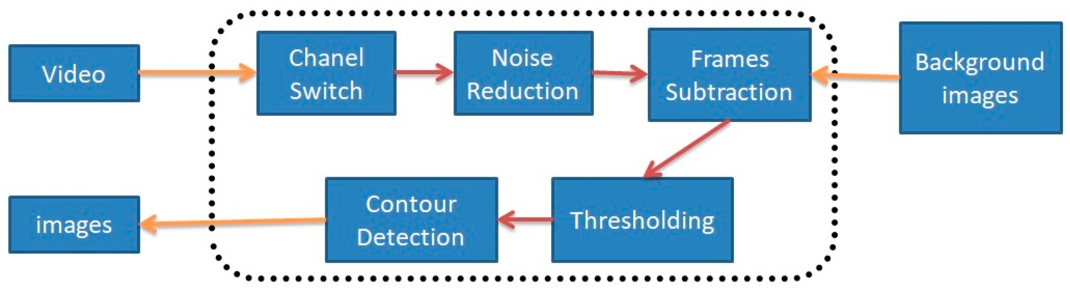
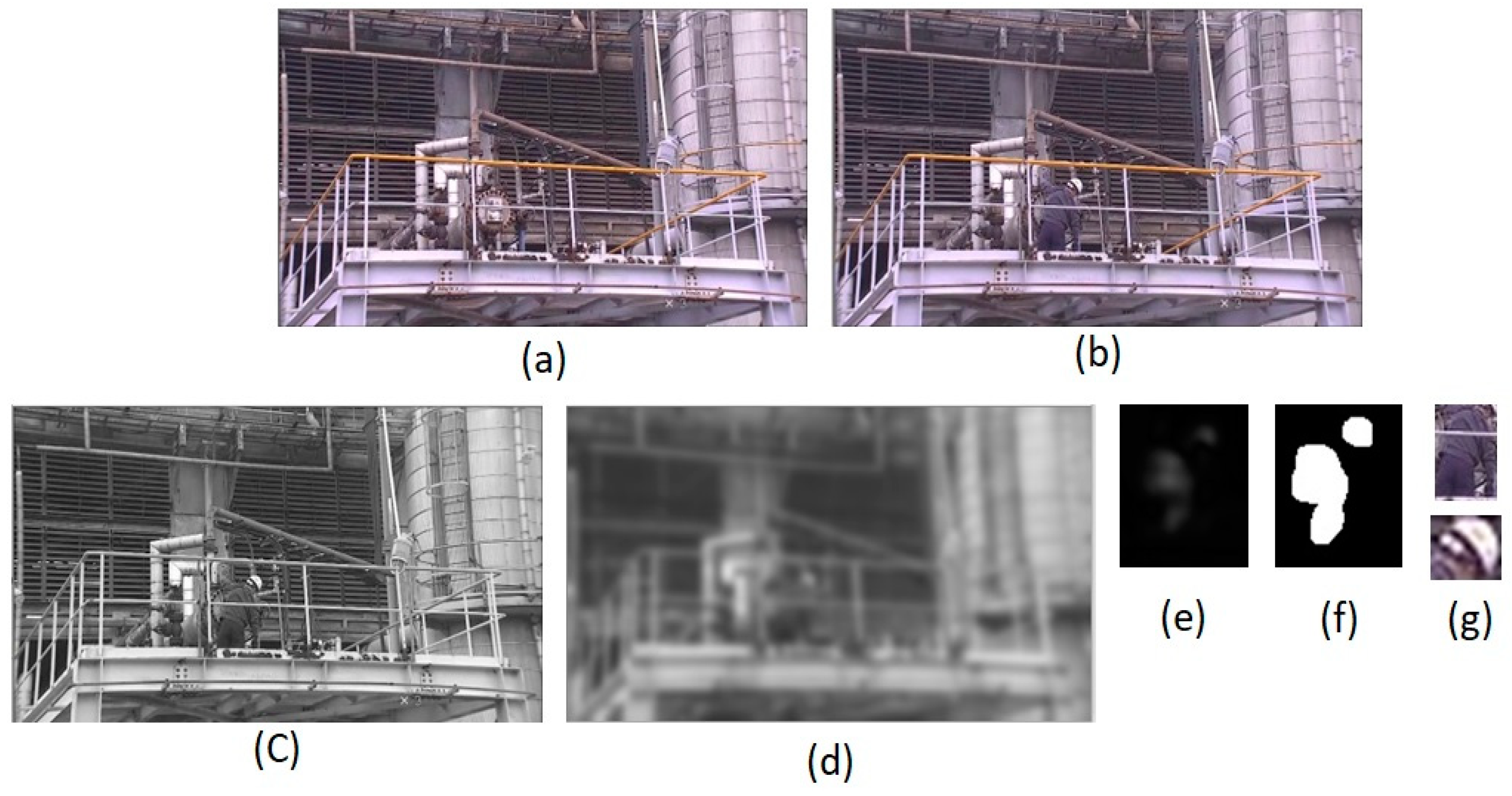
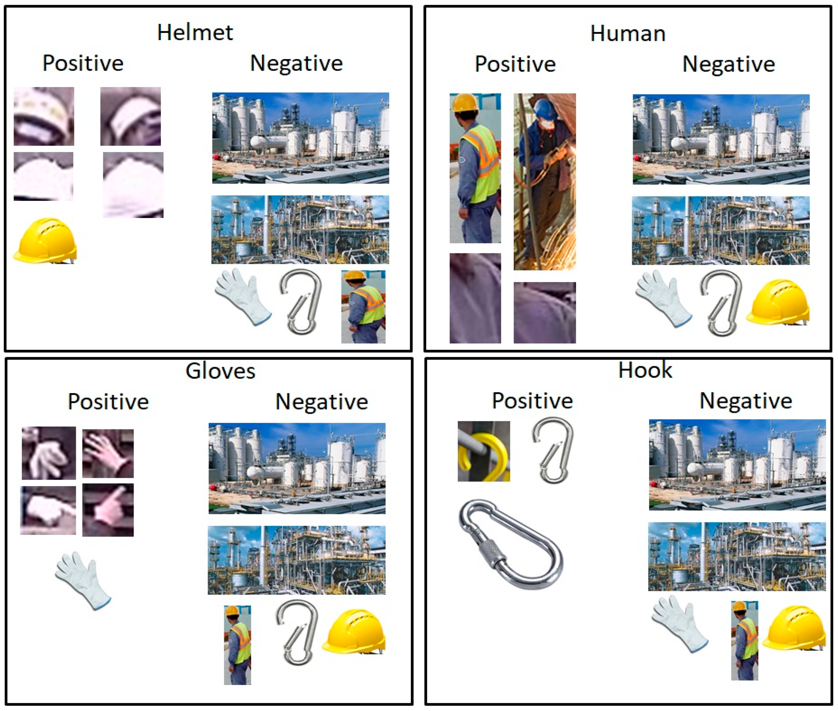
2.2.1. Obtaining Images from Raw Video and Preprocessing and Categorizing Them

This programmed was written in the Python language and ran on an Intel Core i7-6700 CPU—3.40 GHz, with 16 GB RAM and an NVIDIA GeForce GTX 1050 graphics card. This program used the coding library called Open Computer Vision Library (OpenCV) and training libraries from two sources. The first source came from the Open Images Dataset and the second one was from our recorded videos. Initially, the learning step runs before the detecting step. As this algorithm requires a large number of input images, approximately 10 videos were used (30 fps) and some image databases from the internet. These 10 videos were recorded by phone in different backgrounds (school zone, construction zone, and chemical site zone). From the Open Images Dataset, color images of humans, which size varied from 100 × 100 pixels to 200 × 200 pixels were collected. In addition, to collect objects from these videos, motion detection and a tracking algorithm were applied, as shown in Figure 2. These videos have a size of 900 × 500 pixels. In each video, the first background image (no human or safety equipment as in Figure 3a) of three videos is stored before the next frame of the video is processed as the current frame (as Figure 3b). After recording by the computer, the current frame image was applied with color channel switching (from RGB to gray as in Figure 3c) and the Gaussian blur algorithm as Formula 1 (opencv: cv2.cvtColor and cv2.GaussianBlur) (Figure 3d). The idea of Gaussian blur is to use this 2-D distribution as a “point-spread” function, and this point is achieved by convolution. Since the image is stored as a collection of discrete pixels, we need to produce a discrete approximation to the Gaussian function before we can perform the convolution. The Gaussian outputs a “weighted average” of each pixel’s neighborhood, with the average weighted more towards the value of the central pixels. This is in contrast to the mean filter’s uniformly weighted average. Because of this, the Gaussian provides gentler smoothing and preserves edges better than a similarly sized mean filter (blur or median blur). Subsequently, the frame difference between the background frame and current frame is calculated by the function cv2.absdiff, as shown in Figure 3e. The cv2.absdiff is a function that helps in finding the absolute difference between the pixels of the two image arrays. By using this, we will be able to extract just the pixels of the objects that are moving. To use cv2.absdiff we will need to convert our images to grayscale (grayscale is a range of shades of gray ranging from black to white). Based on the frame difference, the dilation of threshold images was found and stored in a basic array (Figure 3f). The threshold binary is a method used in this case as the simplest method to reduce noise [18,19,20]. After that, cv2.findContours functions runs to output these separate shapes appearing in Figure 3f. There are four types of contour: CV_RETR_EXTERNAL, CV_RETR_LIST, CV_RETR_CCOMP, and CV_RETR_TREE. In this case, we use CV_RETR_EXTERNAL to retrieve the extreme outer contours and compress three segments (horizontal, vertical, and diagonal) to only their four ends. Only the shapes with an acceptable size were put out and saved to the computers. This process is shown in Figure 3.

$$\mathrm{G}\left(\mathrm{x},\mathrm{y}\right)=\frac{1}{2{\mathsf{\pi }\mathsf{\sigma }}^2}{\mathrm{e}}^{-\left({\mathrm{x}}^2+{\mathrm{y}}^2\right)/\left(2{\mathsf{\sigma }}^2\right)},$$

(1)

where x is the distance from the origin in the horizontal axis, y is the distance from the origin in the vertical axis, and σ is the standard deviation of the Gaussian distribution.

After the images were obtained, these input images’ sizes were found to vary from 10 × 10 pixels to 200 × 200 pixels. The total images (near three million) were classified to different folders such as helmet, hook, gloves, and human, by hand. The primary need-to-detect objects were helmet, hook, gloves, and people. Therefore, these four required classifiers were used to build the safety system. However, to use the Haar-cascade algorithm, these images were categorized into positive and negative images. A positive image is one containing an object that must be detected; a negative image is one not containing a need-to-find object, as shown in Figure 4. In our case, for example, these positive images of a helmet classifier are helmet images, and the negative ones are hook, human, pipelines, and background. It is similar to the hook, gloves, and human classifiers. To finish the learning step, “good dipping” images were grouped in a folder named “positive”, and “negative” images were grouped in a folder named “negative.”

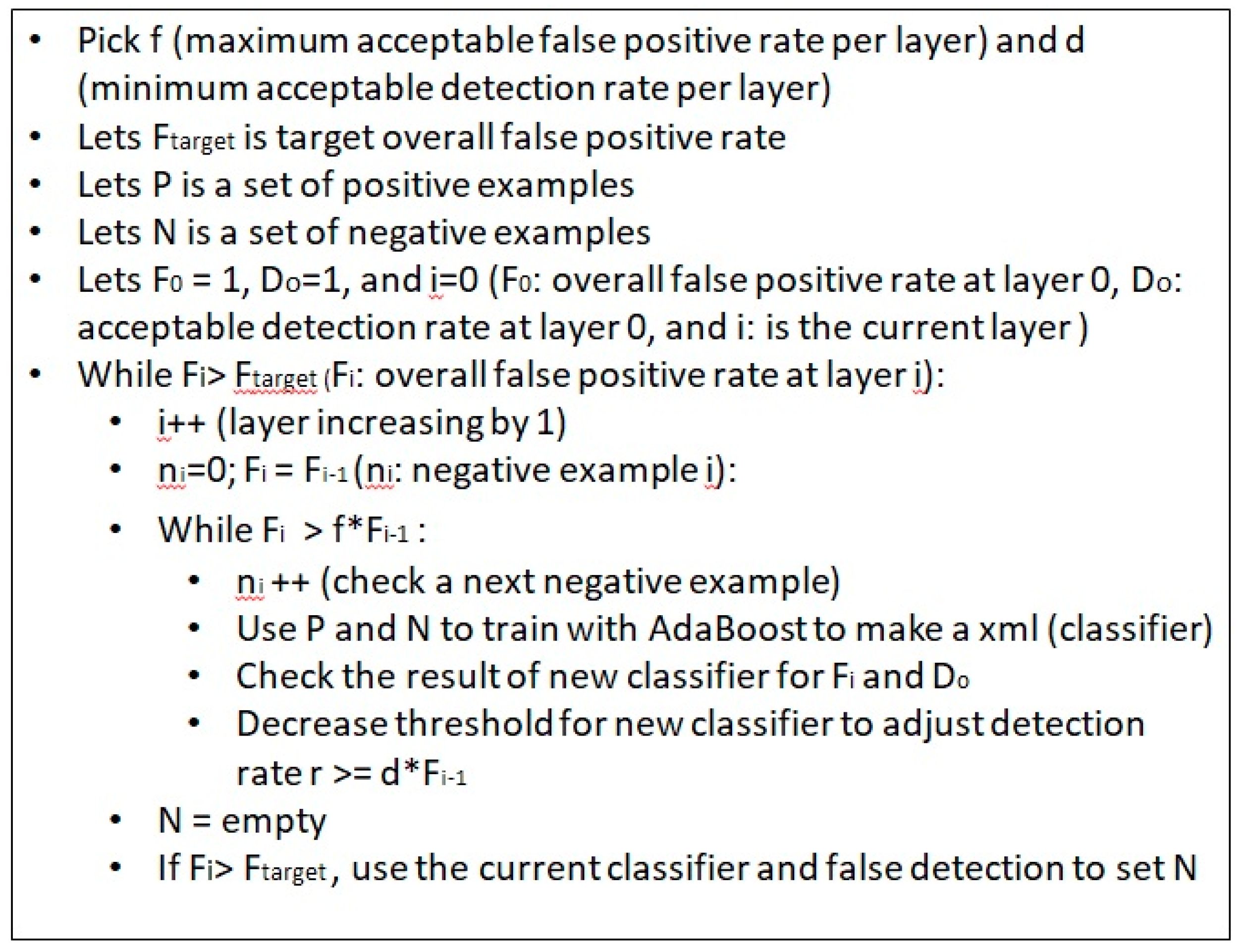
2.2.2. Creating the Haar-Cascade Classifier to Detect Objects

After the procedures in Section 2.2.1 were performed, the couple sets (sets of negative and positive images) were used for creating a classifier of each different object mentioned in the previous section. In this step, the performance is improved from Haar-cascade training by AdaBoost, thus allowing for the algorithm to contain a large number of examples that significantly affects the generalization performance of a strong classifier’s training error. This caused a small number of the images containing the need-to-find object to be misclassified. The AdaBoost algorithm composites with the learning process simultaneously. The purpose of learning was to construct a classifier for the recognition of focus objects. The learning process comprises many states that must be decided by the user. For each state, the computer creates a first classifier from the positive images and tests it on the negative images for evaluation and subsequently builds a second classifier featuring higher detection rates. The second classifier is subsequently used in the next states. This process ends when the last state is completed. The cascade stages are performed by training the classifier tool using the AdaBoost algorithm and compiling with the threshold algorithm to minimize the error rate. The technical input information is listed in

Table 1. Haar-cascade training technical data.

Items	Data/Type
Number of States	20
Number of Threads	7
Acceptance Ratio Break Value	−1
Feature Type	Haar
Haar Feature Type	Basic
Boost Type	GAB
Minimal Hit Rate	0.995
Maximal False Alarm Rate	0.5
Weight Trim Rate	0.95
Maximal Depth Weak Tree	1
Maximal Weak Tree	100
Number of Positives	1150
Number of Negatives	8850

. The number of images for each class is listed in

Table 2. Number of training images for each class.

Helmet (H-Class)		Human (Hu-Class)
Positive	Negative	Positive	Negative
3000	8000	2500	8500
Gloves (G-Class)		Hook (Ho-Class)
Positive	Negative	Positive	Negative
2000	7000	2000	7000

.

When these four completed classifiers of different objects such as the Helmet classifier (H-Class), Glove classifier (G-Class), Hook classifier (Ho-Class), and Human classifier (Hu-Class) were found, the proposed system used them to help AI to maintain the safety level of each object.

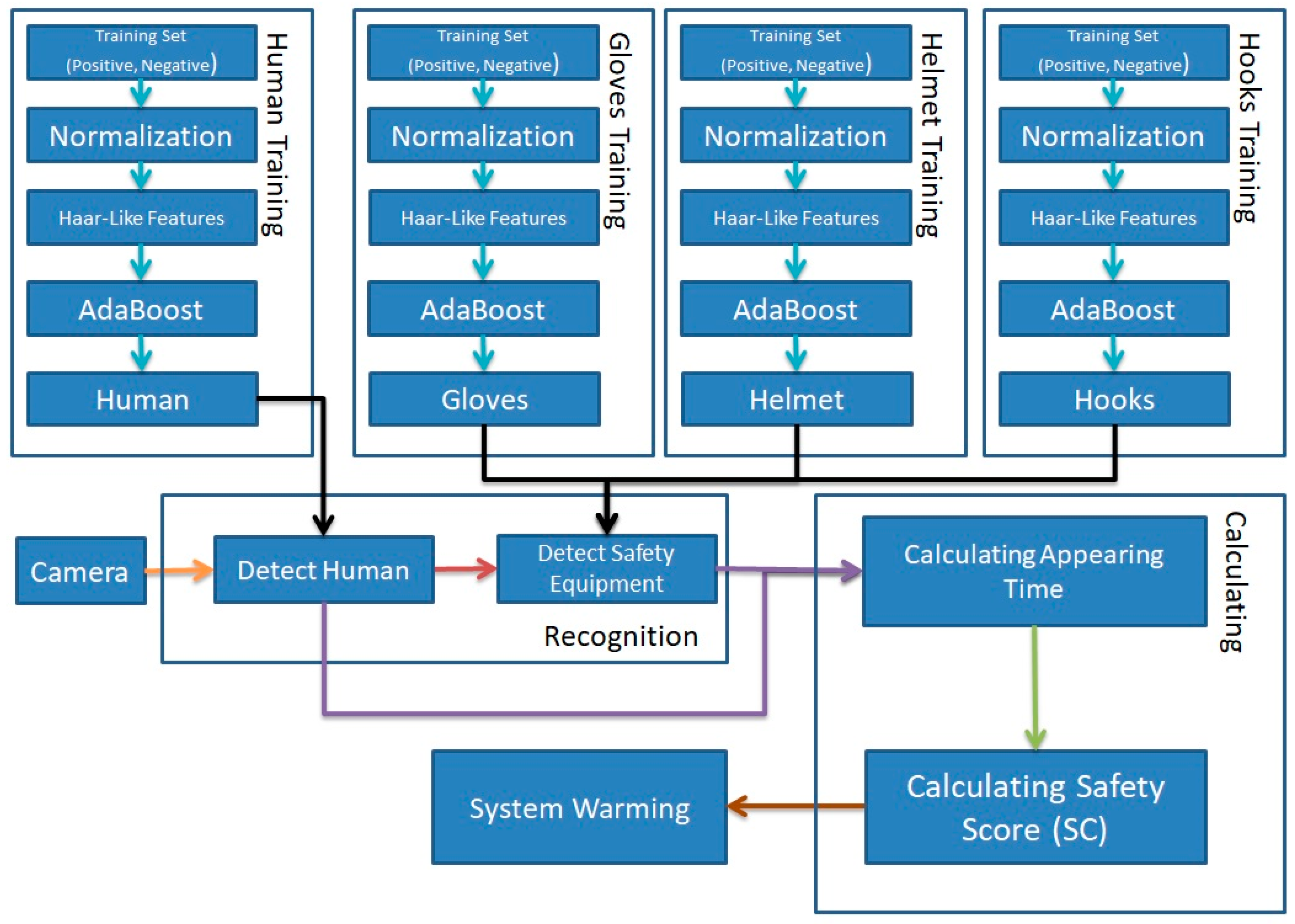
2.2.3. Creating a Safety System for a Chemical Plant Environment

After performing the cascade, a classifier .xml file was generated containing the results of the training process for each class. Four output classifiers were used to detect different objects (helmet, gloves, and hook). To create a safety system, a safety score was calculated based on the scores of the four classes as Equation (2). Each score of H-Class, G-Class, and Ho-Class was based on Equation (3), and the Hu-Score was from Equation (4).

$$\mathrm{SC}\left(\mathrm{x}\right)=S_{Hu}-S_H-S_G-S_{Ho},$$

(2)

where SC(x) is the safety score used to decide whether the system puts an alarm; $S_{Hu}$ is the score of Human; $S_H$ is the score of Helmet;$S_G$ is the score of Gloves; and $S_{Ho}$ is the score of Hook.

$$\mathrm{S}\left(\mathrm{y}\right)=\{\begin{array}{c}0 , when i>h\\ \left(\frac{T}{T^{\prime }}\ast \mathrm{W}\right) , when i\le h\end{array}$$

(3)

where S(y) is the score of the class; T is the difference between the appearing time of an object and that of a human; $T^{\prime }$ is the appearing time of a human; W is the weight value of the object decided by the user based on specific situations; the i is the number of objects; and h is the number of humans.

$${\mathrm{S}}_{Hu}={\displaystyle \sum }_{\mathrm{i}=1}^{\mathrm{n}}{W}_i,$$

(4)

where S_Hu is the score of the Human class and W is the weight value of each class (H-Class, G-Class, and Ho-Class).

For each of the five frames, the system detects the number of humans in the frame; subsequently, if a human is found, $S_{Ho}$,$S_{H }$, and $S_G$ were calculated only when the number of human is higher than the number of detecting objects of each class. The weight value of each class is decided based on the working environment which can be decided later. For example, if the employee works in a scaffolding environment, weight value W of hook can be assigned as 1. And if that person does his job in a ground environment, hook does not need to count, so its W can be 0. But in this research, we decided to have a strong consideration for all of this safety equipment, therefore all of W for class H, G, and Ho were designed as 1. On parallel time, the appearing times of these object were recorded by the Python function “time.time()”. The appearing time of these objects are recorded when the object is found the first time. Based on different situations, $S_{Ho}$,$S_{H }$, and $S_G$ can either be counted or not. Moreover, this system can be flexible to different working environments, such as workers at high places who are required to wear helmets and hooks, or workers at dangerous place who are required to wear gloves. This concept is controlled by the weight value of each class, which is decided by the manager. When SC(x) is found, if it is smaller than a specific value (baseline $\mathrm{SC}\left(\mathrm{x}\right)$), the system will output an alarm signal. This baseline can be established by a user depending on the situation. For example, a school zone does not require a worker to wear safety helmet, hook, or gloves; meanwhile, a chemical site requires these outwear protections strongly. The general concept of our system is shown in Figure 5. The system is programmed in the Python language and tested on a PC with an I7-3770 3.4 GHz processor and 16 GB RAM.

3. Experimental Results

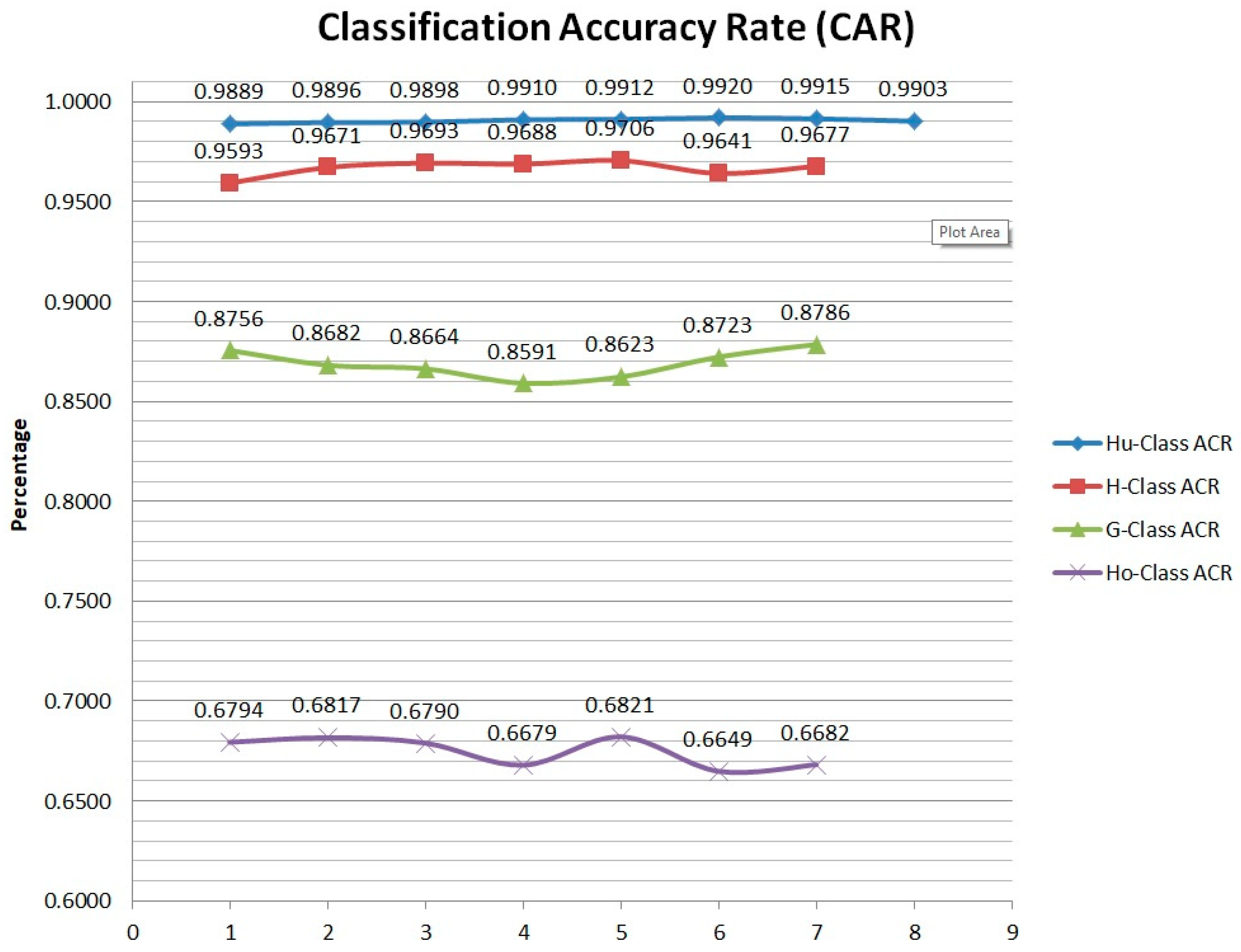
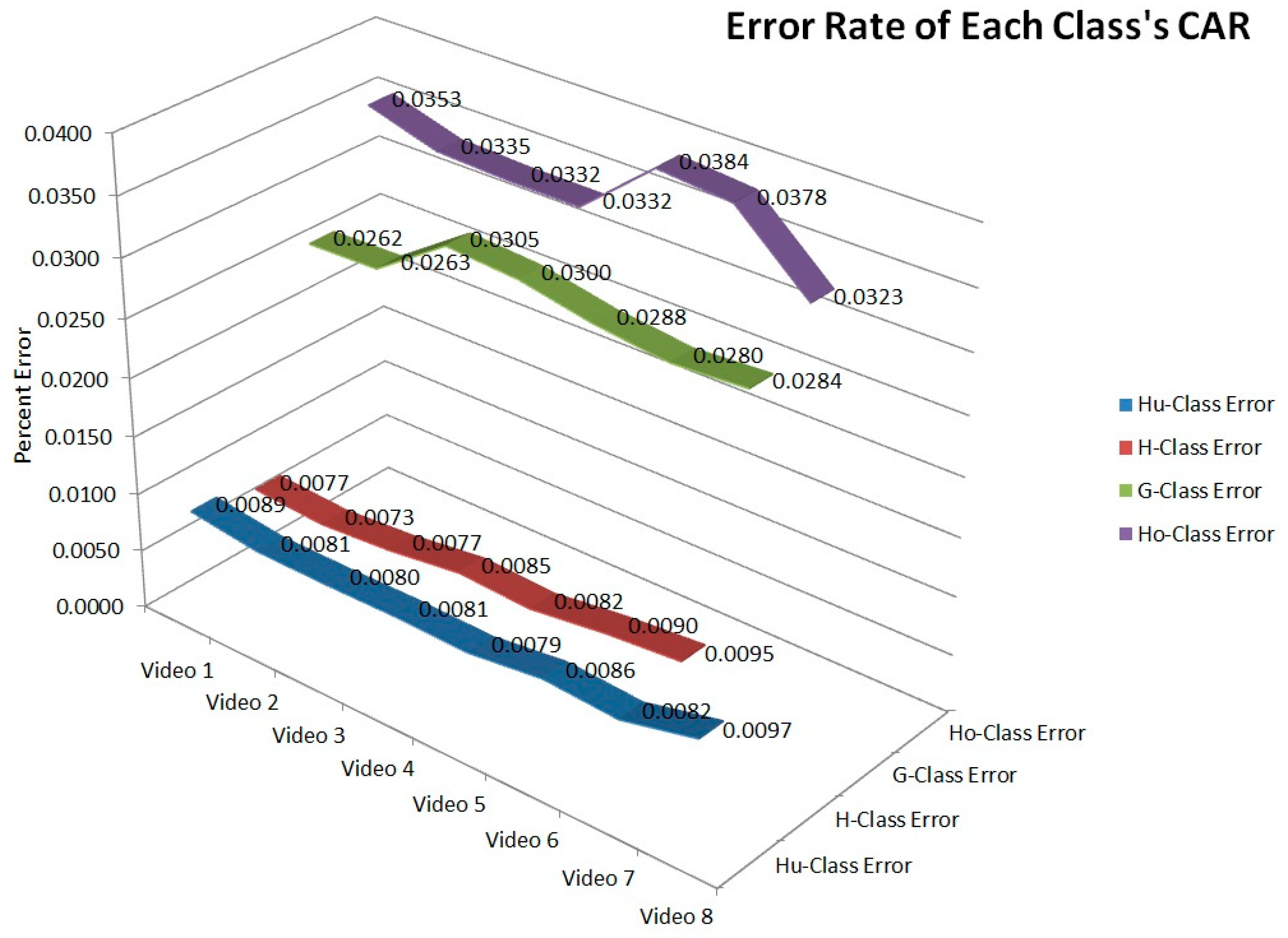
3.1. Performance of Four Class Classifiers

To evaluate the performance of the classifiers, five positive videos, two negative videos, and one background video were used as a test example. Each video is of a different length but the same fps. The three types of video cases were as follows: Positive videos from chemical plants and structure sites containing many workers with safety equipment; negative videos exhibiting people with few or without safety equipment; and background video from normal life with a few humans without any safety equipment. These videos span from 15 to 75 min. For each video case, a single classifier was used to detect its object (H-Class for Helmet, Hu-Class for Human, G-Class for Gloves, and Ho-Class for Hooks). These objects that were found by these classifiers were saved to a PC. The true positive object was that detected by the system as an object of the class and it was an exact object. A false object was detected as an object of the class, but it was not an object (Type-I error). The result of each class classifier is listed in

Table 3. Detection results for each class in eight cases.

No.	No. Frame	Hu-Class		H-Class		G-Class		Ho-Class
		True Positive	False Positive	True Positive	False Positive	True Positive	False Positive	True Positive	False Positive
Video 1 (positive)	28,000	10,325	116	8611	365	19,632	2790	462	218
Video 2 (positive)	54,000	12,233	128	11,069	376	20,051	3045	529	247
Video 3 (positive)	84,000	14,587	151	11,370	360	23,437	3615	531	251
Video 4 (positive)	95,000	14,390	130	12,010	387	22,014	3610	523	260
Video 5 (positive)	108,000	14,104	125	10,590	321	20,110	3211	515	240
Video 6 (negative)	60,000	3100	25	430	16	560	82	123	62
Video 7 (negative)	92,000	3500	30	510	17	680	94	145	72
Video 8 (Background)	45,000	204	2	0	2	0	4	0	1

.

As shown in Table 3, the classification accuracy rate of each classifier is presented as Figure 6. And the error rate of each classifier is presented as Figure 7. These data are calculated from Equation (5). CAR (Classification Accuracy Rate) is a number that can represent the number of correct predictions among all predictions made. It is a good metric when a binary classification problem is encountered (object or non-object). Moreover, to increase the quality of the result, for each case of calculating CAR, a triplicate measurement was performed. Each time yielded a different value and these errors were the average of those differences.

$$\mathrm{CAR}=\frac{\mathrm{Correct}\mathrm{Predictions}}{Total Predictions},$$

(5)

where CAR is the fraction of correct predictions over total prediction, correct predictions are the total correct predictions decided by the system, and total prediction is the total numbers of predictions decided by the system.

In addition, to check the efficiency of this system when using it for a real-time safety management system, a time difference variable is designed to record how fast and how close the system ran comparing with video as Equation (6).

$$\mathrm{Time}\mathrm{difference}=\mathrm{Processing}\mathrm{time}–\mathrm{Video}\mathrm{Time},$$

(6)

where Time difference is decided by a subtraction between processing time and video time. The processing time is calculated by the subtraction between the times when the application start until it ends.

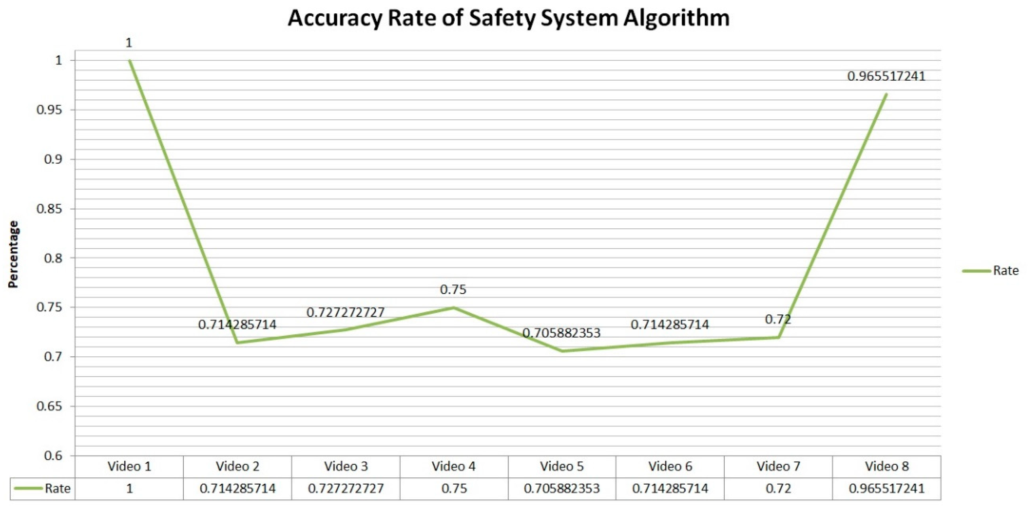
3.2. Performance of the Safety System

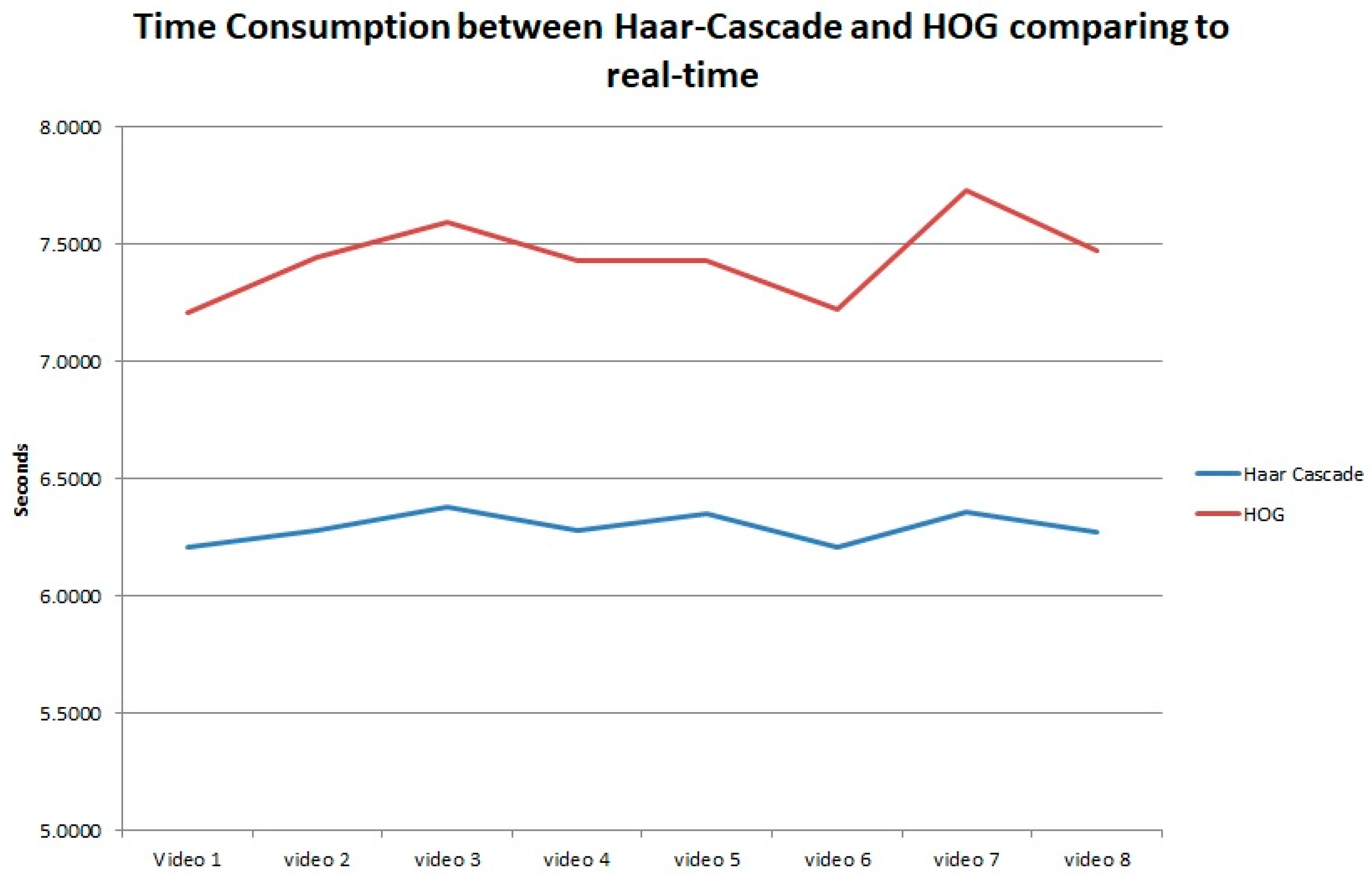
To measure the efficiency of the proposed safety system, eight videos were used. These videos were recorded with different backgrounds such as school zones, chemical plants, and construction sites with people wearing safety equipment or not. In each video, the safety system algorithm (as in Figure 5) was executed several times. Each video exhibits a different number of frames; therefore, it was extremely difficult to store all the safety scores. Hence, the safety score of every frame in every 10 min was stored and the average was calculated. The values in

Table 4. Average safety score of each video at specific times.

	10’	20’	30’	40’	50’	60’	70’	80’
Video 1 (School Zone)	0.683905501	0.837146454	0	0	0	0	0	0
Video 2 (Construction Site)	0.017571454	0.270406121	0.393198	0	0	0	0	0
Video 3 (Construction Site)	0.914408648	0.667811467	0.908317	0.160757	0	0	0	0
Video 4 (Construction Site)	0.149662675	0.10061122	0.649835	0.920592	0.305502	0	0	0
Video 5 (Chemical plant Site)	0.570131747	0.499383685	0.554334	0.560503	0.460353	0.867991	0	0
Video 6 (Chemical plant Site)	0.480631829	0.665851305	0.668991	0.423596	0.077771	0.852459	0.089224	0
Video 7 (Chemical plant Site)	0.656125594	0.212195501	0.203729	0.442033	0.270916	0.342695	0.115809	0
Video 8 (School Zone)	0.632075504	0.754045491	0.277832	0.37724	0.511964	0.845904	0.896601	0.705319

are the average 10 min safety score of each video. The black cell represents the video ending before that milestone. Moreover, the accuracy rate of this safety system was calculated by counting the number of correct times the system underwent a warning over the number of system warnings. For each video, the safety system algorithm was applied thrice to measure the average of the accuracy rate. For each type of video, the baseline $\mathrm{SC}\left(\mathrm{x}\right)$ was decided by the users. If the average safety scores of every 10 min were below the baseline, the system will trigger an alarm. Baseline $\mathrm{SC}\left(\mathrm{x}\right)$ was different in each case (school zone: 0.5; construction site: 0.70; and chemical site: 0.75).

4. Discussion

In Table 3, the number in the frame column represents the length of each video. The number of false positives is smaller than that of positives in all cases, implying that these classifiers performed with high efficiency. Therefore, the CARs of the Hu-Class were from 0.989 to 0.992 (98.9% to 99.2%); for H-Class, the CARs were from 95.6% to 97.1%; for G-Class, the CARs were in the range between 0.859 and 0.877; and, finally, Ho-Class’s CARs varied from 66.8% to 68.2% with very low error rate as Figure 6 and Figure 7. The CAR of Ho-Class is the lowest among the four classes because the object of hook used in these videos from metal, which is typically shivered by sunlight and is extremely difficult to be recorded by any type of camera. Moreover, hooks used in safety must be attached to places that are frequently blocked by pipelines in chemical plant sites or walls. In the G-Class, the numbers of gloves detected by the glove’s classifiers were high because workers must wear gloves when they are working. Any failure (false detection) can be explained by two types of problems such as using insufficient training examples or choosing many training stages. The overall form of cascade classifier resembles a degeneration tree. A positive result from Stage 1 is adjusted and resulted in Stage 2 to achieve a high final detection rate. Finally, in the last case (background video), the number of true positive and false positive examples are insufficient to draw any conclusion. Therefore, we excluded the last case data from the graph.

The error rate of each class demonstrated how the variable spread out the residuals of the algorithm. The error rates were from the difference of each time these classifiers were tested on the videos. This information is an uncertainty of the classifiers over a certain statistic (how our result might differ from the real situation). For example, the CAR of Hu-Class was 98.9% with a 3% difference from a real population point. Figure 8 shows the results of our safety system tested based on eight cases. The cases indicate the average accuracy from 62.5% to 79.3%. The defect might vary based on the quality of the recorded video, the light and shadow of the video, and the complexity of the background image. For example, in test Videos 1 and 8 (school zone), the background was clear, the light and shadow of the video was good, and the complexity was low. Therefore, the accuracy rates of our safety system in these cases were high (over 96%). However, in the other cases, the backgrounds were construction sites and chemical plant sites comprising many pipelines, tubes, and scaffolding that occasionally blocked the objects. To overcome these disadvantages, the system’s camera should be installed at a high location rather than a low location. At a high location, the blocking obstacles will be cleared for object detecting. This will be our future study. Moreover, in Figure 9, the difference between the process time of the system applied to the videos and the real-time video was very slight, around 0.1 min (or 6 s), which is very close to the video’s time and 1 s faster than the system run with HOG. It means that there is a high probability for applying this system in real-time detecting.

5. Conclusions

It is important to maintain the safety of a working environment for workers. Controlling or monitoring the safety score reduces a company, factory, or any organization’s accident rate. Workers are required to wear safety equipment or devices for protection; however, they are occasionally dismissed. Therefore, the safety score system was introduced to detect humans with these protection accessories. Using strong Haar-cascade classifiers from a large number of training sets, the cover setup was programmed to detect humans, helmets, gloves, and hooks as classes with extremely high accuracy (human: 98.9%; helmet: 95.9%; gloves: 85.9%; and hooks: 66.5%) in recorded videos. Furthermore, by recognizing these classes, the safety score of each video at 10’ were calculated and the system warning might signal based on different situations. If this system is applied in real life, a company’s manager can decide a response for different warning situations. With the advantages of the Haar-cascade algorithm, this system can be used as a real-time safety tracking system. Other safety equipment, such as safety masks and safety uniforms, will be reported in our future research. Moreover, in the future work, applying the Haar-cascade algorithm with deep learning will make the system run faster than current deep learning using HOG.

References

1. Slusarczyk, B. Industry 4.0—Are we ready. Pol. J. Manag. Stud. 2018, 17, 232–248. [Google Scholar] [CrossRef]
2. Viola, P.; Jones, M. Robust Real-Time Face Detection, 2001. Int. J. Comput. Vis. 2004, 57, 137–154. [Google Scholar] [CrossRef]
3. Karami, E.; Prasad, S.; Shehata, M. Image Matching Using SIFT, SURF, BRIEF and ORB: Performance Comparison for Distorted Image. In Proceedings of the 2015 Newfoundland Electrical and Computer Engineering Conference, St. John’s, NL, Canada, 5 November 2015. [Google Scholar]
4. Freund, Y.; Schapire, R.E. A Short Introduction to Boosting. J. Jpn. Soc. Artif. Intell. 1999, 14, 771–780. [Google Scholar]
5. Devi, N.S.; Hemachandran, K. Face Recognition Using Principal Component Analysis. Int. J. Comput. Sci. Inf. Technol. 2014, 5, 6491–6496. [Google Scholar]
6. Navaz, A.S.S.; Sri, T.D.; Mazumder, P. Face Recognition Using Principal Component Analysis and Neural Networks. Int. J. Comput. Netw. 2013, 3, 245–256. [Google Scholar]
7. Thakur, S.; Sing, J.K.; Basu, D.K.; Nasipuri, M.; Kundu, M. Face Recognition Using Principal Component Analysis and RBF Neural Networks. In Proceedings of the IEEE First International Conference on Emerging Trends in Engineering and Technology, Nagpur, Nagpur, 16–18 July 2008. [Google Scholar]
8. Wanjale, K.H.; Bhoomkar, A.; Kulkami, A.; Gosavi, S. Use of Haar Cascade Classifier for Face Tracking System in Real Time Video. Int. J. Eng. Res. Technol. 2013, 2, 2348–2353. [Google Scholar]
9. Arreola, L.; Gudino, G.; Flores, G. Object recognition and tracking using Haar-like Features Cascade Classifiers: Application to a quad-rotor UAV. In Proceedings of the 2019 International Conference on Unmanned Aircraft Systems, Atlanta, GA, USA, 11–14 June 2019. [Google Scholar]
10. Cuimei, L.; Zhiliang, Q.; Nan, J.; Jianhua, W. Human Face Detection Algorithm via Haar Cascade Classifier Combined with three additional classifiers. In Proceedings of the IEEE 13th International Conference on Electronic Measurement and Instruments, Yangzhou, China, 20–22 October 2017; pp. 483–487. [Google Scholar]
11. Ulfa, D.K.; Widyantoro, D.H. Implementation of Haar Cascade Classifier for Motorcycle Detection. In Proceedings of the IEEE International Conference on Cybernetics and Computational Intelligence (CyberneticsCom), Phuket, Thailand, 20–22 November 2017. [Google Scholar]
12. Cruz, J.E.C.; Shiguemori, E.H.; Guimaraes, L.N.F. A Comparison of Haar-like, LBP and HOG Approaches to Concrete and Asphalt Runaway Detection in High Resolution Imagery. J. Comput. Int. Sci. 2015, 6, 121–136. [Google Scholar]
13. Arunmozhi, A.; Park, J. Comparison of HOG, LBP and Haar-Like Features for On-Road Vehicle Detection. In Proceedings of the IEEE International Conference on Electro/Information Technology (EIT), Rochester, MI, USA, 3–5 May 2018. [Google Scholar]
14. Guennouni, S.; Ahaitouf, A.; Mansouri, A. A Comparative Study of Multiple Object Using Haar-like Feature Selection and Local Binary Patterns in Several Platforms. Model. Simul. Eng. 2015, 2015, 17. [Google Scholar] [CrossRef]
15. Qi, F.; Li, H.; Luo, X.; Ding, L.; Rose, T.; An, W. Detecting Non-hardhat-use by a Deep Learning method from Far-field Surveillance Videos. Autom. Constr. 2018, 85, 1–9. [Google Scholar]
16. Ge, Y.; Zhang, R.; Wu, L.; Wang, X.; Tang, X.; Lou, P. Deepfashion2: A versatile Benchmark for Detection, Pose Estimation, Segmentation and Re-Identification of Clothing Images. arXiv 2019, arXiv:1901.070973. [Google Scholar]
17. Yang, M.; Yu, K. Real-Time Clothing Recognition in Surveillance Videos. In Proceedings of the 18th IEEE International Conference on Image Processing, Brussels, Belgium, 11–14 September 2011; pp. 2937–2940. [Google Scholar]
18. Senthilkumaran, N.; Vaithegi, S. Image Segmentation by Using Thresholding Techniques for Medical Images. Comput. Sci. Eng. Int. J. 2016, 6, 1–13. [Google Scholar]
19. Bulent, S.; Sezgin, M. Image thresholding techniques: A survey over categories. Pattern Recognit. 2001, 34, 1573–1583. [Google Scholar]
20. Sezgin, M.; Sankur, B.; Bebek, I. Survey Over Image Thresholding Techniques. J Electron. Imaging 2004, 13, 146–168. [Google Scholar]
Figure 1. Haar-cascade algorithm pseudo code.
Electronics 08 01079 g001
Figure 2. Motion- and object-tracking algorithm diagram.
Electronics 08 01079 g002
Figure 3. Obtaining images examples: (a) first background image; (b) current frame image; (c) grayscale image of (b); (d) Gaussian blur image of (c); (e) frame subtraction using cv2.absdiff image; (f) threshold image of (e); and (g) result image achieved from (f).
Electronics 08 01079 g003
Figure 4. Positive and negative image examples.
Electronics 08 01079 g004
Figure 5. Safety system process diagram.
Electronics 08 01079 g005
Figure 6. Classification rate of each class.
Electronics 08 01079 g006
Figure 7. Error rate of CAR.
Electronics 08 01079 g007
Figure 8. Accuracy rate of the algorithm.
Electronics 08 01079 g008
Figure 9. Time difference between the video ran with the Haar cascade and with the histogram of object gradients (HOG).
Electronics 08 01079 g009