Abstract
As a key ingredient of deep neural networks (DNNs), fully-connected (FC) layers are widely used in various artificial intelligence applications. However, there are many parameters in FC layers, so the efficient process of FC layers is restricted by memory bandwidth. In this paper, we propose a compression approach combining block-circulant matrix-based weight representation and power-of-two quantization. Applying block-circulant matrices in FC layers can reduce the storage complexity from to . By quantizing the weights into integer powers of two, the multiplications in the reference can be replaced by shift and add operations. The memory usages of models for MNIST, CIFAR-10 and ImageNet can be compressed by , and with minimal accuracy loss, respectively. A configurable parallel hardware architecture is then proposed for processing the compressed FC layers efficiently. Without multipliers, a block matrix-vector multiplication module (B-MV) is used as the computing kernel. The architecture is flexible to support FC layers of various compression ratios with small footprint. Simultaneously, the memory access can be significantly reduced by using the configurable architecture. Measurement results show that the accelerator has a processing power of 409.6 GOPS, and achieves 5.3 TOPS/W energy efficiency at 800 MHz.
1. Introduction
Deep neural networks (DNNs) have been widely applied to various artificial intelligence (AI) applications [1,2,3,4] and achieve great performance in many tasks such as image recognition [5,6,7], speech recognition [8] and object detection [9]. To complete the tasks with higher accuracy, larger and more complex DNN models emerge and become increasingly popular. Large scale DNNs, however, require massive parameters and high computation complexity. For instance, there are 138 million weights and 15.5 billion multiply-accumulate (MAC) operations in VGG-16 for image recognition [10]. As a result, the implementation of these DNN models is challenging for portable devices with restricted computational capability and memory resources.
Fully-connected (FC) layers are applied in various deep learning systems. Neurons in an FC layer have connections to all activations in the previous layer, making FC layers the most memory intensive in large DNN networks. For example, 96% and 90% of weights storage are taken by FC layers in AlexNet and VGG-16, respectively. In models that only consist of FC layers, there can be billions of parameters [11]. The efficient process of FC layers is mainly limited by bandwidth in large networks [12]. Thus, it is essential to reduce the memory access of FC layers, especially when they are deployed in embedded devices containing limited hardware resources.
Several network compression techniques have been proposed to reduce the redundant parameters in DNNs. Targeting the compressed networks, hardware accelerators have been proposed to process DNNs with higher performance and energy efficiency. Focusing on pruning-based technique [13], a corresponding hardware accelerator has been developed in [12]. By exploiting the sparsity of both weights and activations, the weights are stored in a compressed format to save memory usage and unnecessary computations are removed. The pruning-based technique, however, leads to irregular network structure and unbalanced computation [12]. In [14,15,16,17], quantization for weights with low precision has been explored. Although bringing some accuracy loss, quantization remains an efficient way to reduce the weight memory size and improve the energy efficiency of DNN hardware. In [18,19,20], DNN accelerators based on binary weights have been proposed.
Using structured matrices to explore the redundancy of DNNs is another efficient technique. Circulant matrix-based methods can provide good compression ratio for weights, and Fast Fourier Transformation (FFT) can be employed to reduce the computational complexity [21,22,23,24]. In [24], block-circulant matrices are employed in FC layers and the circulant matrix-vector multiplications are accelerated by FFT-based methods in both the training and inference. Compared with pruning-based approach in [13], this method avoids irregular sparse network structure and inefficient implementation of activations and indices. Liao et al. [25] proposed block-circulant matrix-based DNN training and inference schemes, as well as an optimized FFT-based hardware architecture. Compared with prior work, this approach achieves significantly improvement in energy efficiency. However, using FFT and IFFT transformation limits the quantization of weights. To achieve good balance between the hardware performance and precision loss in FFT-based method, at least 12 bits are required to represent a weight. In addition, additional computation components are needed to perform FFT and IFFT.
In this paper, an efficient compression technique for fully-connected layers is proposed. We employ block-circulant matrix-based method to compress the network weight matrices and further quantize each entry in weight matrices to an integer power of two. For block-circulant matrix-based FC layers with low precision weights, a configurable hardware accelerator, called BPCA, is proposed. The main contributions of the paper are summarized as follows.
- (1)
- An efficient compression technique combining block-circulant matrices and power-of-two quantization for fully-connected layers is proposed. This approach can significantly save the networks’ storage usage. Specifically, we directly train the FC layers in DNN models with block-circulant matrices and the storage requirement can be reduced from to . Based on the above models, we further quantize each entry in weight matrices to an integer power of two. The computational complexity can be significantly reduced because the multiplications in the forward pass can be replaced by shift operations.
- (2)
- An efficient, configurable and scalable hardware architecture is proposed for the compressed networks. Instead of FFT-based acceleration methods, we design this architecture to take advantage of the circular feature of weight matrices and power-of-two quantization. Notably, multipliers are replaced by customized processing elements (PEs) using shift and add operations. Due to the adjustable sizes of block-circulant matrices, we design a configurable hardware architecture. A reorganization scheme is used to realize the configurability of layers and reduce the parameters’ memory access.
- (3)
- Experiments on several datasets (MNIST, CIFAR10, and ImageNet) are presented to prove the general applicability of the proposed approach. According to our experiments, 4 bits are enough to represent the weights, thus quantization provides eight times additional compression ratio. The proposed hardware architecture was also implemented and evaluated. The implementation results demonstrate that the proposed design has high energy efficiency and area efficiency.
2. Background
2.1. Computation of FC Layers
Matrix-vector multiplication (MV) is the key computation in FC layers in the DNN inference. The computation in an FC layer is performed as follows
where x is the input activation vector; y is the output activation vector; is the weight matrix of this layer in which b input nodes connect with a output nodes; is the bias vector; and is the nonlinear activation function and the Rectified Linear Unit (ReLU) is widely adopted in various DNN models.
The space complexity and computational complexity of an FC layer are . In practice, the values of a and b in an FC layer can be large and there is no data reuse, so the computation of FC layers is memory intensive. For many neural network architectures, the memory access is the bottleneck to process FC layers efficiently.
2.2. Block-Circulant Matrix
A circulant matrix can be defined by a primitive vector , which is the first row of the circulant matrix:
If a matrix is composed of a set of circulant sub-matrices (blocks), it is defined as a block-circulant matrix [24]. A block-circulant matrix can be expressed by
where is a circulant sub-matrix and can be represented with a primitive vector of length k. Thus, if a normal matrix is transformed into a block-circulant matrix, the numbers of parameters to be stored can be reduced by k times.
3. Proposed Compression Method
The approach to present weight matrices of DNNs using block-circulant matrices is proposed in [24], where an FFT-based acceleration method is applied to accelerate the inference and training. Instead of the FFT-based method, we propose to employ the power-of-two quantization in the block-circulant matrix-based DNNs to further reduce the storage requirement and computational complexity. This section describes the proposed compression method combining block-circulant matrix-based weight representation and power-of-two quantization.
3.1. Block-Circulant Matrix-Based FC Layers
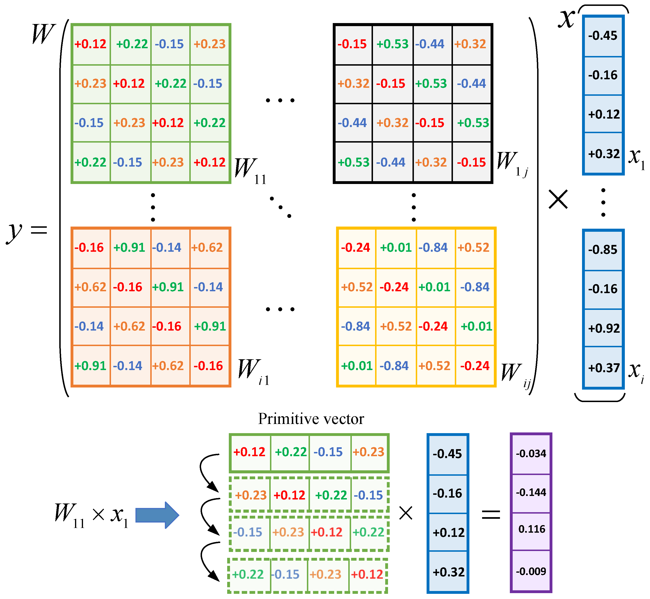
When a block-circulant matrix is applied in an FC Layer, the original weight matrix can be represented by 2D blocks of square sub-matrices, where each sub-matrix is a circulant matrix. Assume that the weight matrix W is partitioned into sub-matrices and the block size (size of each sub-matrix) is denoted by k. Here, and . Then, , , , and assume that the primitive vector of is . Simultaneously, the input vector is divided into q sub-vectors and then , where . Then, the in Equation (1) is given by (with bias and ReLU omitted):
where and .
Figure 1 illustrates the representation approach. A weight matrix is partitioned into circulant sub-matrices and the block size is 4. Then, the result of can be computed by the multiplications of sub-matrices and corresponding sub-vectors. As described in Section 2.2, only the primitive vector of each sub-matrix need to be stored, so the storage complexity of an FC layer will be reduced from () to .
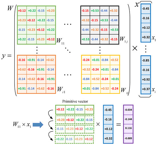
Figure 1.
Block-circulant matrices representation for FC Layers.
Because of the flexible size of block-circulant matrix, the compression ratio is adjustable and determined by the block size. Larger block size brings better compression ratio, but there will be more accuracy loss. On the contrary, smaller block size provides higher prediction accuracy, but the compression ratio may degrade. Notably, block-circulant matrix-based DNNs have been proven to asymptotically approach the accuracy of original networks using theoretical analysis [26].
For the training of block-circulant matrix-based DNNs, the corresponding training algorithm based on backward propagation is proposed in [24]. In this work, we do not use FFT in the inference and training, so we remove FFT from the training algorithm in [24]. The compressed DNNs are directly trained with block-circulant matrix-based weights, where no retrain process is required.
3.2. Power-of-Two Quantization
Suppose that a DNN model, which uses block-circulant matrices in FC layers, is pre-trained with full-precision weights. We propose to represent each entry in the weight matrix with an integer power of two. Thus, the weight matrix W can be approximated by a low-precision weight matrix , and each entry of is defined by
where n is an integer and sign function is used to decide the sign of . Here, n is calculated by
where , and are two integers, and . Thus, all the entries of can be selected from a codebook set
If we use b-bit indices to represent the entries of , there are total combinations of indices. To determine the value of , we can find the maximal entry of and then use Equation (6) to calculate . The minimum value of can be determined by . For example, we use 4 bit indices and the values of original weights are limited in . Then, is 0 and the minimal value of is . Thus, the codebook set . Then, we use the 4-bit indices to encode each entry of .
Since all entries are quantized into integer powers of two, the multiplications in the can be replaced by shift operations. The computational complexity in the inference can be significantly reduced and no multipliers are required.
3.3. Training and Quantization Strategy
A two-stage training process combining block-circulant matrix-based weight representation and retrain-based quantization strategy is proposed. Algorithm 1 describes the training process. In the first stage, block-circulant matrices are employed in FC layers of a DNN model. Specifically, primitive vectors of the sub-matrices in FC layers are randomly initialized with normal distribution. Then, other parameters in the block-circulant matrices are generated by using the primitive vectors. Next, we train the network with the block-circulant matrix-based training algorithm. In the second stage, based on the pre-trained model, we further quantize the weights with power-of-two scheme, and then retrain the network with quantized parameters. At the same time, the network weight matrices are still represented with block-circulant matrices.
| Algorithm 1 Training strategy with block-circulant matrices and weight quantization. PoT() is power-of-two quantization and C is the loss function. |
| Input: A minibatch of inputs I, targets , previous weights and previous learning rate . Output: Updated weights and updated learning rate 1: Quantize the original weights: 2: = PoT () 3: //Forward propagation with the quantized parameters in block-circulant weight matrices 4: = PoTBackward //Backward propagation with the quantized weights 5: // Update the original weights with respect to 6: // Update the learning rate |
4. Efficient Hardware Architecture
As shown in Figure 2, the weight matrix of an arbitrary FC layer can be represented by circulant matrices, where and denote the row number and column number of blocks in the weight matrix, respectively. According to Equation (4), the MV in the computation of an FC layer can be partitioned into multiplications of circulant sub-matrices and sub-vectors. Each can be computed independently and then the results of in the same row can be accumulated to get the corresponding result vector . All the multiplications can be replaced by shift operations by using the quantization scheme proposed in Section 3.2. To take full advantage of the quantization scheme, we do not use the FFT-based acceleration method in [24] because: (1) FFT-based method limits the quantization of weights. In [24], the accuracy is low, if the weights are quantized to 4 bits. (2) If the weights are transformed by FFT, we cannot use shift-operations to remove multiplications.
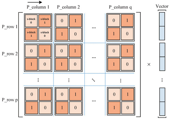
Figure 2.
Computing scheme for an FC layer.
As shown in Figure 2, the weight matrix of an arbitrary FC layer can be represented by circulant matrices, where and denote the row number and column number of blocks in the weight matrix, respectively. According to Equation (4), the MV in the computation of an FC layer can be partitioned into multiplications of circulant sub-matrices and sub-vectors. Each can be computed independently and then the results of in the same row can be accumulated to get the corresponding result vector . All the multiplications can be replaced by shift operations by using the quantization scheme proposed in Section 3.2. To take full advantage of the quantization scheme, we do not use the FFT-based acceleration method in [24] because: (1) FFT-based method limits the quantization of weights. In [24], the accuracy is low, if the weights are quantized to 4 bits. (2) If the weights are transformed by FFT, we cannot use shift-operations to remove multiplications.
4.1. Reorganization of Block-Circulant Matrix
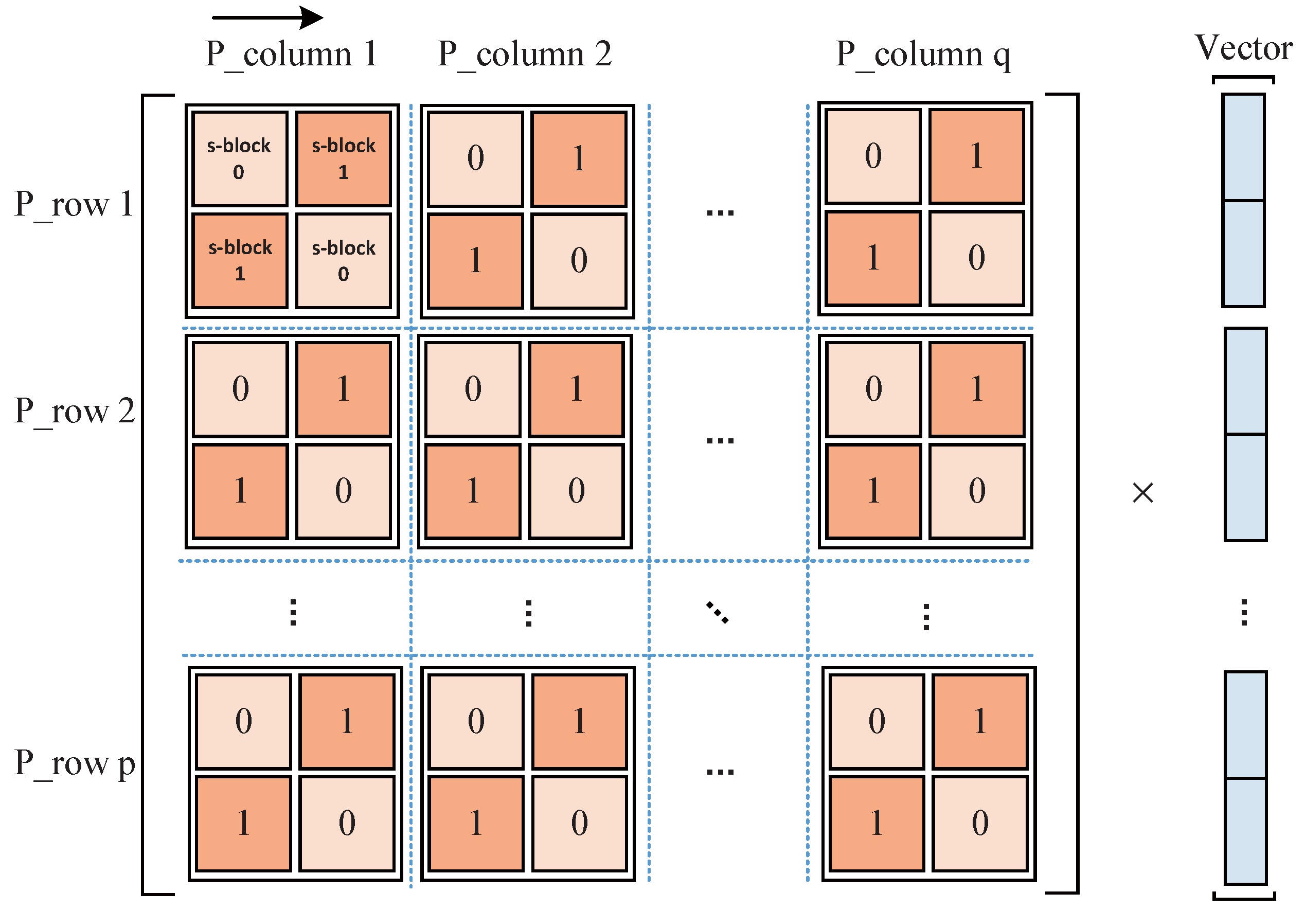
We can directly compute the sub-matrix and sub-vector multiplications when the block size is small. However, when the block size is large, e.g., 256 × 256, directly computing the is inefficient. In addition, because of the variable block size, a configurable hardware architecture is required. Thus, we propose to further divide every sub-matrix into smaller sub-blocks, each of which is still a circulant matrix. Similar chessboard division method is proposed in [27] for each sub-matrix. Figure 2 shows an example of the division, where each sub-matrix is partitioned into four sub-blocks. Specifically, we use a reorganization scheme [27] in each sub-matrix to further transform it into a block pseudocirculant matrix [28,29]. The detailed transformation scheme is illustrated as follows.
We assume that a sub-matrix is partitioned into sub-blocks, each of which is by () short circulant matrix denoted by :
where . Correspondingly, vector is divided into small vectors denoted by , where , .
The circulant matrix vector multiplication (C-MV) can be represented as follows
where is the cyclic shift operator matrix
Then, we can compute in parallel and , . For example, is given by
Each in the polynomial in Equation (11) is a C-MV and can be computed separately.
4.2. Architecture of Block-MV
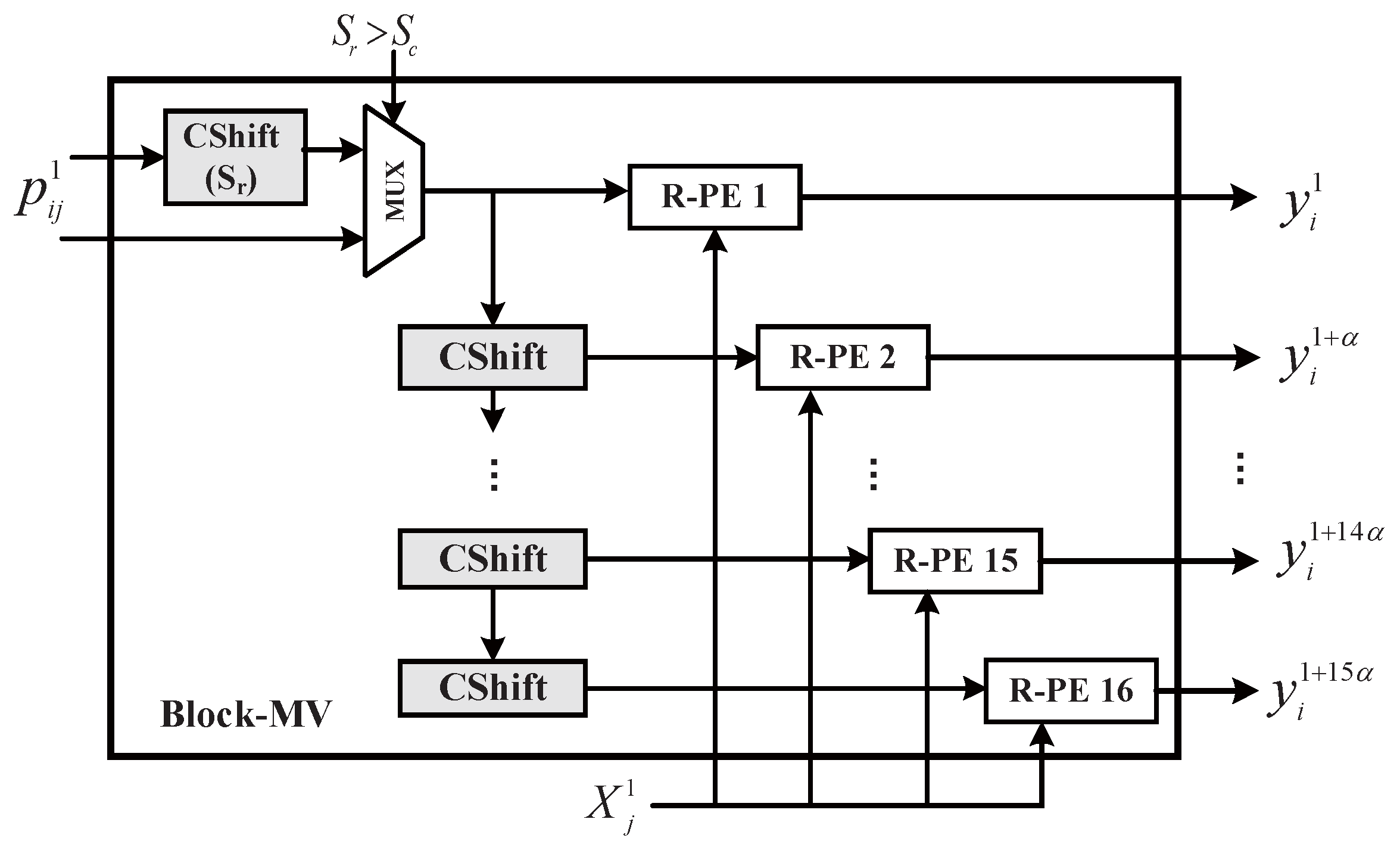
Using the reorganization scheme in Section 4.1, we can transform a sub-matrix into smaller sub-blocks. By observing the block size, we set the as the basic size of a sub-block, because all block sizes in our experiment were the multiples of 16. If the block size is , we can directly compute the C-MV. If the block size is larger than 16, the matrix can be naturally reorganized into several sub-blocks. As shown in Figure 3, the Block-MV (B-MV) module is the key computing module for processing the short C-MV, . Suppose the block size and . Then, can be represented as follows
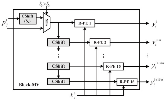
Figure 3.
Architecture of Block-MV.
When computing , and the primitive vector of , will first be fetched. Then, the primitive vector will be shifted to form the other rows in . and are parameters to denote the row and column of each sub-block. If , needs an additional left shift to implement the function of . Then, the activation vector and corresponding weight vectors will be sent to 16 row processing elements (R-PEs) to compute dot products in parallel.
When is computed, and will be prepared by a read controller (R-ctrl). After the calculation is finished, will be computed in the B-MV and the result will be accumulated in R-PEs. Next, and will be computed successively. When computation of C-MVs in the first row is finished, the result will be sent to an accumulator module. It is the same for computing , , and in the B-MV. Finally, when the B-MV finishes all the C-MVs of one sub-matrix, it will start the processing for the following sub-matrix. With the parallel processing of R-PEs, a sub-block can be processed in 1 clock, so clocks are required to compute a sub-matrix.
4.3. Row Processing Element
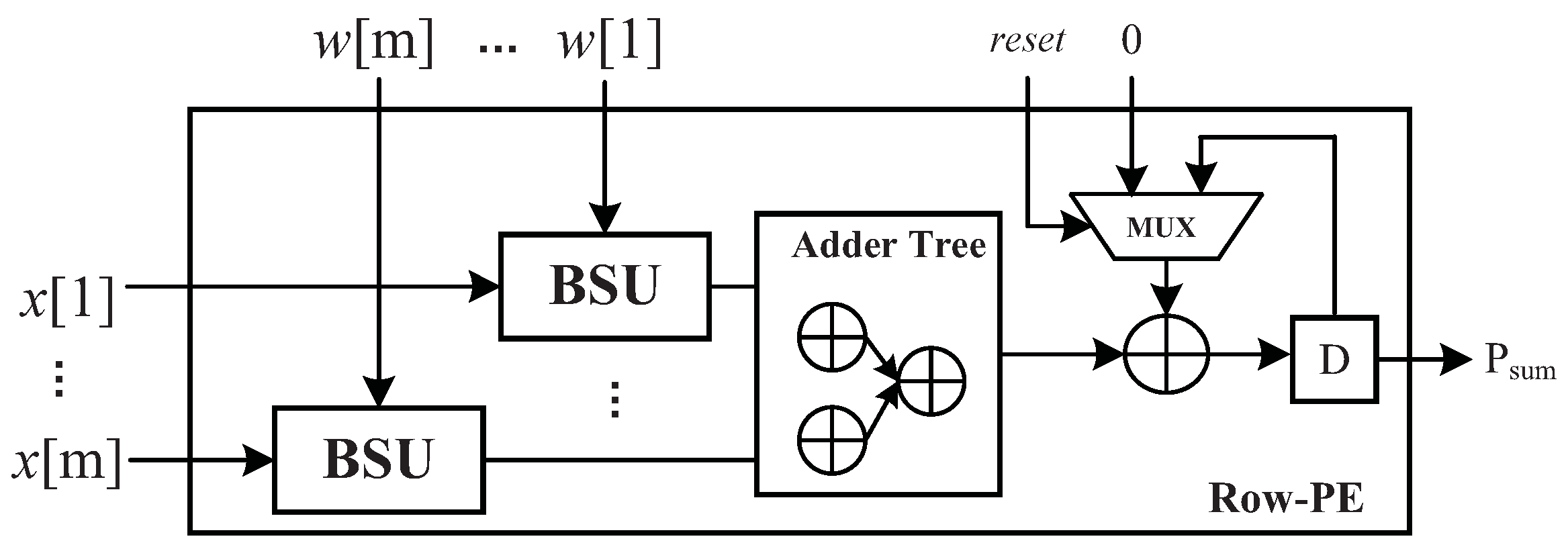
As shown in Figure 4, R-PEs are basic processing elements in the B-MV and each R-PE can compute m MACs in parallel. The mathematical representation of an R-PE’s output is
where is a weight parameter and is an element of an activation vector. Since the multiplications are replaced by shift operations, the element-wise multiplication of and is implemented with a basic shift unit (BSU) instead of a multiplier. The BSU performs shift operations on according to the weight indices. As values of the weights are limited in , only the left-shift operations are required. In a weight index, the highest bit denoted by is the sign bit, and the other bits in the index are the shift bits, . The value of determines the shift bits performed on . Table 1 shows the shift operations of a BSU with 4-bit indices.

Figure 4.
Architecture of row processing element.

Table 1.
Weight indices and shift operations in a BSU.
After is computed by the adder trees, the partial sum is stored in a register and accumulated every clock cycle. The reset signal in Figure 4 works when current partial sum is sent to the accumulator module for further processing.
4.4. Configurable Hardware Accelerator Architecture
The overall architecture of BPCA is shown in Figure 5. To fit for the adjustable block size and various network sizes of FC layers, BPCA is designed to provide flexibility for different needs. In general, designing a configurable accelerator involves the considerations of several factors: , the block size of one sub-matrix; , the row number of sub-matrices in a weight matrix; , the column number of sub-matrices in a weight matrix; and , the number of accumulators in the Accumulator module. According to the configuration parameters, the configurable controller (Config-ctrl) controls the computing of other components in BPCA. Weights, bias, and input activations are stored in three different SRAMs, which are W-RAM, B-RAM and A-RAM in Figure 5, respectively. The weights and input vectors are sent to the B-MV by the read-controller (Read-ctrl) according to different . The output vectors of all the sub-matrices in one row will be accumulated in the Accumulator module. In the following, we describe the configurable scheme in detail.

Figure 5.
Hardware accelerator architecture for FC layers.
For different FC networks, the BPCA requires configurable parameters including , and . As described in Section 4.2, the Block-MV can process a fixed-sized sub-block for one time. According to , the Read-ctrl feeds the 16-by-16 sub-blocks and corresponding activations to the Block-MV for processing. When all sub-blocks in one sub-matrix are processed, the Config-ctrl will move on to the calculation of the next sub-matrix in the same sub-matrix row. As shown in Figure 2, BPCA performs a row-wise computing scheme. Thus, according to , the Config-ctrl needs to judge whether current sub-matrix is the last one in current sub-matrix row. If the sub-matrix is the last one, the in the Accumulator module will be sent to the Bias-ReLU module for further processing, and then the final result vector of one sub-matrix row will be output. Because the size of a sub-matrix is adjustable, is determined by the biggest number of that BPCA supports. Since the size of output vector of each sub-matrix row is changeable, the Config-ctrl selects accumulators in the Accumulator module in every computing procedure.
As the main computing element, B-MV determines the processing time of an FC layer and the system throughput. In addition, the proposed hardware architecture is scalable, and the system throughput can be improved by adding more B-MVs.
5. Experiments of The Proposed Compression Method
We verified the effectiveness of the proposed method on three standard datasets: MNIST, CIFAR-10, and ImageNet. We compared the accuracy and storage cost of the compressed neural network models and the original neural network models. Since the effectiveness of applying block-circulant matrices in FC layers has been proven in [24,25], we pay more attention to the effectiveness of power-of-two quantization on the block-circulant matrix-based FC layers. To test quantization precision’s influence on prediction accuracy, we selected different for and quantized the weights with different quantization precision. Notably, the aim of our experiment was not to seek the state-of-the-art results on these datasets, thus the accuracy of the original neural networks was only used as a baseline for a fair comparison with the compressed neural networks.
5.1. Experiments on MNIST
MNIST is a digit dataset that contains 28 × 28 grey-scale images of ten handwritten digits (0 to 9). In MNIST, there are 60,000 images for training and 10,000 images for testing. The baseline model that we used is a three-layer DNN denoted by Model-A. The matrix sizes and parameters of the FC layers in Model-A are shown in Table 2. We tested the proposed compression methods on Model-A and the training results are given in Table 3. We first applied block-circulant matrices () in FC1 and FC2 layers. Then, we quantized the weights under different quantization precision. When , the quantization precision is and weights can be represented with 3 bits. Thus, quantization provides 10.7 times compression ratio (compared with 32-bit floating point). Other quantization precision requires 4-bit indices and the storage cost can be saved by eight times. We can see that quantization precision has little effect on the prediction accuracy. As a result, block size of 16 and 3-bit quantization can compress the FC layers by 170 times with accuracy loss.
Table 2.
FC Layers in the models for MNIST, CIFAR, and ImageNet.
Table 3.
Experiment results of Model-A for MNIST.
5.2. Experiments on CIFAR
CIFAR-10 dataset contains 60,000 natural 32 × 32 RGB images covering 10-class objects. There are 50,000 images for training and 10,000 images for testing. In our test, the network consisted of six convolutional layers and three fully-connected layers [18]. ReLU was used as the activation function. The proposed compression method was used in FC4 and FC5 layers. We also selected different to test the accuracies under different quantization precision, which is shown in Table 4. There is negligible accuracy loss when weights are quantized into 3 or 4 bits. Thus, the FC layers can be compressed by 2731× with 0.8% accuracy loss.
Table 4.
Experiment results of Model-B for CIFAR-10.
5.3. Experiments on ImageNet
We further evaluated the effectiveness of the proposed compression methods on the ImageNet ILSVRC-2012 dataset, which contains images of 1000 categories of objects. There are roughly 1000 images in each of the 1000 considered categories. AlexNet [5] was used as the baseline model denoted by Model-C, which consisted of five convolutional layers, two FC layers and one final softmax layer. The Top-1 accuracy and Top-5 accuracy of Model-C are and , respectively. The FC layers of Model-C are shown in Table 2. We applied block-circulant weight matrix in FC7, FC8 and FC9 layers with sub-matrices. Then, the weights were quantized with 4 bits. The length of output vector in FC9 was not a multiple of 16, thus we added eight rows at the end of the weight matrix to make it a 4096 × 1008 matrix. Then, the network could be trained as normal, but the eight additional outputs were dropped to get the results of 1000 categories that we wanted. As shown in Table 5, the network can be compressed by 128 times with accuracy loss. When power-of-two quantization is used in large scale networks, there is more accuracy loss compared with small networks.
Table 5.
Experiment results of Model-C for ImageNet.
5.4. Result Analysis
The power-of-two quantization scheme is effective when it is combined with block-circulant matrix-based weight representation on the three models. In general, the accuracy of a network is dominated by the block size of weight matrices. To achieve a trade-off between accuracy and compression ratio, the block size of each layer should be adjusted carefully. Quantization causes minimal accuracy loss on MNIST, CIFAR-10 and ImageNet, when the weights are quantized into 4 bits with precision 1/64.
6. Hardware Implementation Results
We evaluated the performance of the hardware architecture proposed in Section 4. The RTL of the design was implemented in Verilog and synthesized by using the Synopsys Design Compiler (DC) under the TSMC 40 nm CMOS technology. We measured the area, power, and critical path delay of the accelerator. Benchmarks were obtained from Models A–C.
6.1. Evaluation Results and Analysis
The synthesis results of the top architecture are presented in Table 6. A frequency of 800 MHz has been achieved. In our design, the basic size of a sub-block can be processed is . One B-MV containing 16 R-PEs is used for processing sub-blocks. The synthesis results of the R-PE are presented in Table 6.
Table 6.
Synthesis results of the proposed hardware architecture (logic part) and row processing element.
The on-chip SRAM consisted of W-RAM, A-RAM, and B-RAM. Notably, since the accelerator needed to process different scale networks, the SRAM sizes were selected to suitable for large scale FC layers. The on-chip SRAM was modeled using Cacti [30] under 45 nm process. In our design, 16 bits and 4 bits were used to represent activations and weights, respectively. The A-RAM was for storing activations, where the maximum input length of activations was 9216. The width of W-RAM was 64 bits and the size of W-RAM aws 1.747 MB. Thus, all compressed weights in FC layers of AlexNet could be stored in W-RAM. In addition, we used 16 bits to represent biases and B-RAM was , where the maximum number of biases was 4096.
The power/area breakdown of the accelerator is presented in Table 7. BPCA occupies 12.72 mm, where the memory dominates the chip area with of the total area. The logic part of BPCA only occupies 0.16 mm. The total power consumption is 77.09 mW and the memory consumes 24.13 mW.
Table 7.
Synthesis results of the breakdown by module (LINE 2-3) of the accelerator. The critical path is 1 ns.
6.1.1. Performance
To measure the performance of BPCA, we defined throughput () as the input numbers per seconds. is dominated by the B-MV and is given by
In our design, is 16 and = 800 MHz, thus numbers/s. The bigger the is, the smaller the input throughput is, which means less memory access is required. As for the computing performance, the giga operations per second (GOPS) is 409.6 GOPS corresponding to an uncompressed layer.
The computation time to process one weight matrix in the steady stage is
Nine pipeline stages are introduced in the design, so the actual runtime of one layer requires an additional nine clock cycles.
We selected benchmarks from Model-A, Model-B, and Model-C to evaluate performance of the accelerator. Layers A–E had different matrix sizes and block sizes. The configuration parameters and computation time are shown in Table 8. It takes 184.32 s to process layer C, which is the largest FC layer in AlexNet. To process middle scale layers, such as Layers A and B, only a few microseconds are consumed.
Table 8.
Benchmarks from three different DNN models.
6.1.2. Flexibility and Scalability
BPCA can fit for different scale FC layers with adjustable compression ratios. In this experiment, the could be configured to 16, 32, 64, 128, and 256. The basic sub-block size, which is processed by a B-MV, can be changed according to different requirements.
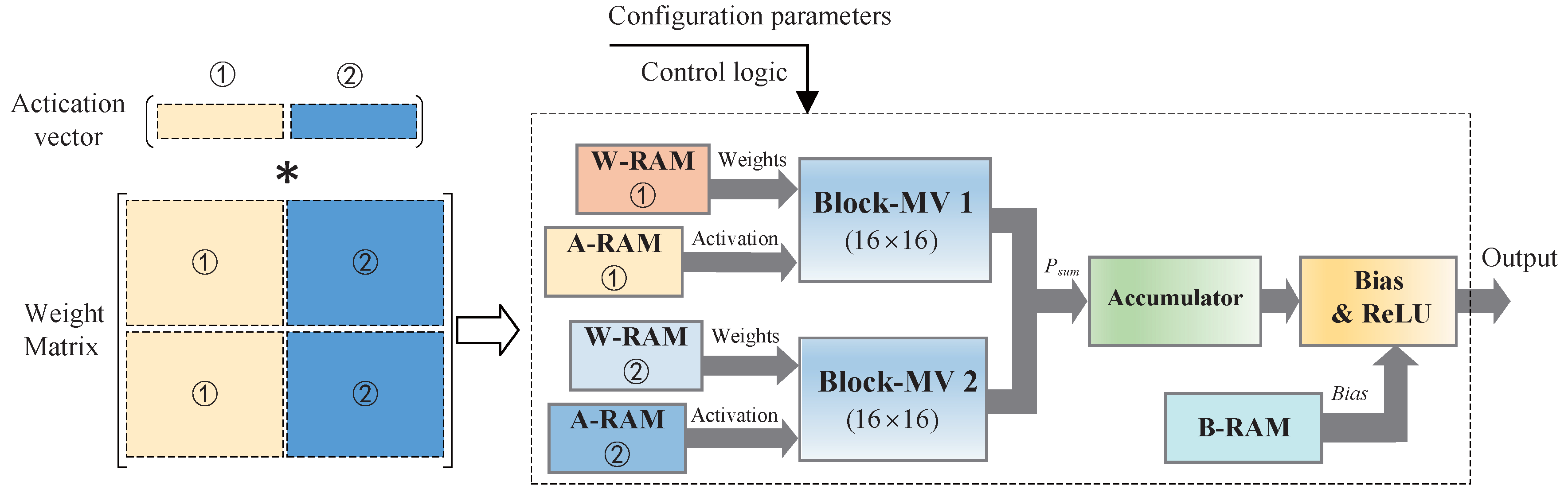
To fit for larger weight matrices, BPCA can be scaled up by adding more B-PEs. As shown in Figure 6, a large weight matrix can be divided into two parts and the corresponding parameters are stored in different weight RAMs. The two-part weight matrices can be processed by two B-MVs in parallel. To further improve the system throughput, more B-MVs can be used in the system.
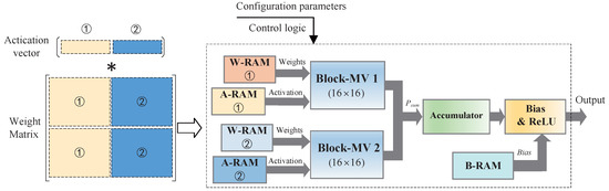
Figure 6.
The scalability of the accelerator.
6.2. Comparisons with Related Works
Based on FPGA or ASIC platforms, numerous works on DNN accelerators have been proposed. We compared BPCA with representative state-of-the-art ASIC development and synthesis results. Table 9 shows the comparisons with accelerators focusing on compressed networks or uncompressed networks.
Table 9.
Comparisons with state-of-the-Art DNN accelerators.
EIE [12] is a representative accelerator for processing sparse DNNs. EIE is mainly composed of customized PEs focusing on sparse matrix-vector multiplications. The computations of a network are partitioned for different PEs to perform and every PE stores a partition of the network in local SRAM. The FC layers of AlexNet can fit into 64 PEs in EIE. Using the same benchmark, AlexNet, we compared our work with EIE composed of 64 PEs.
In one PE of EIE, there are on-chip memory in sparse matrix read unit, activation read/write and pointer read unit for decoding the compressed weights. The memory takes 93.22% of the PE’s area. The arithmetic unit in a PE performs multiply-accumulate operations by using one multiplier and one adder. Running at 800 MHz, the logic part of one PE takes an area of 43,258 m, resulting in area efficiency of 37 GOPS/mm. The basic processing element in BPCA is R-PE. One R-PE can perform 16 multiply-accumulate operations in parallel using 16 adders and no multipliers. Because there are no additional decoding process, the area of an R-PE is dominated by computing units. As shown in Table 7, at 800 MHz, an R-PE takes 6944 m, resulting in area efficiency of 3.7 TOPS/mm. Without multipliers and decoding units, R-PE achieves significantly higher area efficiency than the PE of EIE.
In EIE, the sparse weight matrices, which are encoded in compressed sparse column (CSC) format, can all be stored in on-chip SRAM. With the encoding format, additional 4-bit indices and pointer vectors are required for the decoding of compressed weight matrices. The weight SRAMs of 64 PEs is 8 MB and can hold 4-bit weights and 4-bit indices of AlexNet’s FC layers with at least 8× weight sparsity. Each PE has a pointer SRAM and the total SRAM capacity for pointers is 2 MB. In addition, the activation SRAM in each PE is 2 KB and 64 PEs use 128 KB SRAM for activations. The on-chip SRAM dominates the area in EIE and takes of the total area of EIE. At 800 MHz, EIE (64 PEs) can yield a performance of 102 GOPS and the area efficiency can achieve 2.5 GOPS/mm (including SRAM). In BPCA, the accelerator also stores the FC layers of AlexNet in SRAM. Using block-circulant matrix, the weight matrix can be compressed by 16×. By using power-of-two quantization, the weights can be represented with 4 bits. Storing the block-circulant matrix-based layers does not require indices or pointers such as storing the sparse matrices in EIE. Without using additional indices, 2× storage usage can be reduced. In addition, 2 MB storage can be saved by using no pointers. In the accelerator, the weight SRAM is 1.772 MB and the activation SRAM is 18 KB. The on-chip SRAM takes 98.76% of BPCA’s area. For the same benchmark, AlexNet, BPCA can achieves an area efficiency of 31.8 GOPS/mm, which is 13× of EIE.
Our work also outperforms EIE in energy efficiency. In one PE of EIE, the memory consumes of the total power. Sixty-four PEs use 10.125-MB SRAM, which consumes 348 mW. Compared with EIE, we use less SRAM and save 14× power of memory. The logic part of one EIE’s PE consumes 3.74 mW, but the power of R-PE is only 57.5% of EIE’s PE. As shown in Table 9, the energy efficiency of BPCA can achieve 5.3 TOPS/W, which is 31× of EIE.
DNPU [31] is configurable heterogeneous accelerators supporting CNNs, FCLs, and RNNs. We mainly compare BPCA with the part of DNPU on FC layers. The weights in DNPU can be quantized into 4–7 bits using dynamic fixed point. However, without other compression method, the parameters of DNPU are still required to be fetched from external memory (DRAM). By using the proposed compression method, our work can save much more DRAM access than DNPU. Besides, one compressed FC layer can be stored in on-chip SRAM, which consumes less energy than storing parameters in off-chip memory. In DNPU, quantization table-based matrix multiplication is used and 99% of the 16-bit fixed-point multiplications can be avoided. At 200 MHz, the energy efficiency of DNPU can achieve 1.1 TOPS/W. BPCA also does not use any multipliers and can achieve 5 TOPS/W at 800 MHz. Compared with DNPU, our work achieves competitive performance and energy efficiency with less memory access.
7. Conclusions
In this paper, we present an effective compression method and an efficient configurable hardware architecture for fully-connected layers. Block-circulant matrices and power-of-two quantization are employed in this approach to compress the DNNs. Block-circulant matrices provide an adjustable compression ratio for weight matrices by changing the block size. Using power-of-two quantization, we can represent the weights with low precision and reduce computational complexity by replacing the multiplications with shift operations. The approach was applied to three classic datasets and provided remarkable compression ratios. For MINIST, the FC layers can be compressed by 171× with 1% accuracy loss. The results on CIFAR-10 show that the FC layers can be compressed by 2731× with negligible accuracy loss. Our experiment on ImageNet compresses the weight storage of AlexNet by 128× with 1.8% accuracy loss. The proposed compression method outperforms pruning-based method in compression ratio and avoids irregular computations of pruned networks.
To process the compressed neural network efficiently, we develop a configurable, area-efficient and energy-efficient hardware architecture, BPCA. BPCA can be configurable to process FC layers with different compression ratios. Without using multipliers, a lot of chip area can be saved in R-PEs and system throughput can be significantly improved. The proposed design is implemented under the TSMC 40 nm CMOS technology. Using 1.772-MB SRAM, the accelerator can do 409.6 GOPS in an area of 12.72 mm and dissipates 77.09 mW. Our work outperformed pruning-based accelerator, EIE [12], in energy efficiency by 31× and area efficiency by 13×.
8. Discussion
In this paper, the proposed compression scheme targets FC layers. In the experiments for Model B and Model C, we only applied the proposed compression method in FC layers and the accuracy of Model C has already shown some reduction on Imagenet dataset. Since FC layer has a lot of redundancy, the quantization may cause minimal accuracy loss. As for convolutional layers, which are sensitive to quantization, the proposed method may cause much accuracy loss. Thus, the quantization scheme should be examined carefully in block-circulant matrix-based CNNs. In our future work, we will evaluate the proposed method on convolutional layers and explore better quantization schemes on block-circulant matrix-based CNNs.
Author Contributions
Conceptualization, H.P. and Z.Q.; methodology, Z.Q. and D.Z.; software, D.Z.; validation, X.Z. and X.C.; formal analysis, Z.Q.; investigation, X.Z.; resources, H.P. and L.L.; data curation, X.Z. and X.C.; writing—original draft preparation, Z.Q.; writing—review and editing, Z.L. and Y.S.; visualization, Z.Q.; supervision, H.P. and Y.G.; project administration, Q.S.; and funding acquisition, H.P., Y.S. and Y.G.
Funding
This research was funded in part by the National Nature Science Foundation of China under Grant No. 61376075 and 41412020201, in part by the key Research and Development Program of Jiangsu Province under Grant No. BE2015153, and in part by the Priority Academic Program Development of Jiangsu Higher Education Institutions(PAPD).” “The APC was funded by the National Nature Science Foundation of China under Grant No. 61376075”.
Acknowledgments
This work was supported in part by the National Nature Science Foundation of China under Grant No. 61376075 and 41412020201, in part by the key Research and Development Program of Jiangsu Province under Grant No. BE2015153, and in part by the Priority Academic Program Development of Jiangsu Higher Education Institutions(PAPD).
Conflicts of Interest
The authors declare no conflict of interest.
References
- Tang, Z.L.; Li, S.M.; Yu, L.J. Implementation of Deep Learning-Based Automatic Modulation Classifier on FPGA SDR Platform. Electronics 2018, 7, 122. [Google Scholar] [CrossRef]
- Liu, X.; Yang, T.; Li, J. Real-Time Ground Vehicle Detection in Aerial Infrared Imagery Based on Convolutional Neural Network. Electronics 2018, 7, 78. [Google Scholar] [CrossRef]
- Wang, X.; Hua, X.; Xiao, F.; Li, Y.; Hu, X.; Sun, P. Multi-Object Detection in Traffic Scenes Based on Improved SSD. Electronics 2018, 7, 302. [Google Scholar] [CrossRef]
- Nguyen, T.V.; Mirza, B. Dual-layer kernel extreme learning machine for action recognition. Neurocomputing 2017, 260, 123–130. [Google Scholar] [CrossRef]
- Krizhevsky, A.; Sutskever, I.; Hinton, G.E. Imagenet classification with deep convolutional neural networks. In Proceedings of the International Conference on Neural Information Processing Systems, Lake Tahoe, NV, USA, 3–8 December 2012; pp. 1097–1105. [Google Scholar]
- Simonyan, K.; Zisserman, A. Very deep convolutional networks for large-scale image recognition. In Proceedings of the International Conference on Learning Representations, Banff, AB, Canada, 14–16 April 2014; pp. 1–14. [Google Scholar]
- Mirza, B.; Kok, S.; Dong, F. Multi-layer online sequential extreme learning machine for image classification. In Proceedings of ELM-2015 Volume 1; Springer: Berlin, Germany, 2016; pp. 39–49. [Google Scholar]
- Mikolov, T.; Karafiát, M.; Burget, L.; Černockỳ, J.; Khudanpur, S. Recurrent neural network based language model. In Proceedings of the International Symposium on Computer Architecture, Saint-Malo, France, 19–23 June 2010; pp. 1045–1048. [Google Scholar]
- Dominguez-Sanchez, A.; Cazorla, M.; Orts-Escolano, S. A New Dataset and Performance Evaluation of a Region-Based CNN for Urban Object Detection. Electronics 2018, 7, 301. [Google Scholar] [CrossRef]
- Sze, V.; Chen, Y.H.; Yang, T.J.; Emer, J.S. Efficient processing of deep neural networks: A tutorial and survey. Proc. IEEE 2017, 105, 2295–2329. [Google Scholar] [CrossRef]
- Dean, J.; Corrado, G.S.; Monga, R.; Chen, K.; Devin, M.; Le, Q.V.; Mao, M.Z.; Ranzato, M.; Senior, A.; Tucker, P.; et al. Large Scale Distributed Deep Networks. In Proceedings of the International Conference on Neural Information Processing Systems, Lake Tahoe, NV, USA, 3–8 December 2012; pp. 1223–1231. [Google Scholar]
- Han, S.; Liu, X.; Mao, H.; Pu, J.; Pedram, A.; Horowitz, M.A.; Dally, W.J. EIE: Efficient Inference Engine on Compressed Deep Neural Network. In Proceedings of the International Symposium on Computer Architecture, Seoul, Korea, 18–22 June 2016; pp. 243–254. [Google Scholar] [CrossRef]
- Han, S.; Mao, H.; Dally, W.J. Deep compression: Compressing deep neural networks with pruning, trained quantization and huffman coding. In Proceedings of the International Conference on Learning Representations, San Juan, Puerto Rico, 2–4 May 2016. [Google Scholar]
- Courbariaux, M.; Bengio, Y. BinaryNet: Training Deep Neural Networks with Weights and Activations Constrained to +1 or −1. arXiv, 2016; arXiv:1602.02830. [Google Scholar]
- Wu, J.; Leng, C.; Wang, Y.; Hu, Q.; Cheng, J. Quantized convolutional neural networks for mobile devices. In Proceedings of the International Conference on Computer Vision and Pattern Recogintion, Las Vegas, NV, USA, 26 June–1 July 2016; pp. 4820–4828. [Google Scholar]
- Choi, Y.; El-Khamy, M.; Lee, J. Towards the limit of network quantization. In Proceedings of the International Conference on Learning Representations, San Juan, Puerto Rico, 2–4 May 2016. [Google Scholar]
- Courbariaux, M.; Bengio, Y.; David, J.P. BinaryConnect: Training Deep Neural Networks with binary weights during propagations. In Proceedings of the International Conference on Neural Information Processing Systems, Montreal, QC, Canada, 7–12 December 2015; pp. 3123–3131. [Google Scholar]
- Zhao, R.; Song, W.; Zhang, W.; Xing, T.; Lin, J.H.; Srivastava, M.; Gupta, R.; Zhang, Z. Accelerating binarized convolutional neural networks with software-programmable fpgas. In Proceedings of the 2017 ACM/SIGDA International Symposium on Field-Programmable Gate Arrays, Monterey, CA, USA, 22–24 February 2017; ACM: New York, NY, USA, 2017; pp. 15–24. [Google Scholar]
- Ando, K.; Ueyoshi, K.; Orimo, K.; Yonekawa, H.; Sato, S.; Nakahara, H.; Takamaeda-Yamazaki, S.; Ikebe, M.; Asai, T.; Kuroda, T.; et al. BRein memory: A single-chip binary/ternary reconfigurable in-memory deep neural network accelerator achieving 1.4 TOPS at 0.6 W. IEEE J. Solid-State Circuits 2018, 53, 983–994. [Google Scholar] [CrossRef]
- Wang, Y.; Lin, J.; Wang, Z. An energy-efficient architecture for binary weight convolutional neural networks. IEEE Trans. Very Large Scale Integr. (VLSI) Syst. 2018, 26, 280–293. [Google Scholar] [CrossRef]
- Cheng, Y.; Felix, X.Y.; Feris, R.S.; Kumar, S.; Choudhary, A.; Chang, S.F. Fast neural networks with circulant projections. arXiv, 2015; arXiv:1502.03436. [Google Scholar]
- Cheng, Y.; Yu, F.X.; Feris, R.S.; Kumar, S.; Choudhary, A.; Chang, S.F. An exploration of parameter redundancy in deep networks with circulant projections. In Proceedings of the International Conference on Computer Vision and Pattern Recogintion, Boston, MA, USA, 7–12 June 2015; pp. 2857–2865. [Google Scholar]
- Sindhwani, V.; Sainath, T.; Kumar, S. Structured transforms for small-footprint deep learning. In Proceedings of the International Conference on Neural Information Processing Systems, Montreal, QC, Canada, 7–12 December 2015; pp. 3088–3096. [Google Scholar]
- Ding, C.; Liao, S.; Wang, Y.; Li, Z.; Liu, N.; Zhuo, Y.; Wang, C.; Qian, X.; Bai, Y.; Yuan, G.; et al. Circnn: Accelerating and compressing deep neural networks using block-circulant weight matrices. In Proceedings of the 50th Annual IEEE/ACM International Symposium on Microarchitecture, Cambridge, MA, USA, 14–18 October 2017; ACM: New York, NY, USA, 2017; pp. 395–408. [Google Scholar]
- Liao, S.; Li, Z.; Lin, X.; Qiu, Q.; Wang, Y.; Yuan, B. Energy-efficient, high-performance, highly-compressed deep neural network design using block-circulant matrices. In Proceedings of the 36th International Conference on Computer-Aided Design, Irvine, CA, USA, 13–16 November 2017; IEEE Press: Piscataway, NJ, USA, 2017; pp. 458–465. [Google Scholar]
- Zhao, L.; Liao, S.; Wang, Y.; Tang, J.; Yuan, B. Theoretical Properties for Neural Networks with Weight Matrices of Low Displacement Rank. CoRR 2017. Available online: http://xxx.lanl.gov/abs/1703.00144.
- Wang, Z.; Lin, J.; Wang, Z. Accelerating Recurrent Neural Networks: A Memory-Efficient Approach. IEEE Trans. Very Large Scale Integr. (VLSI) Syst. 2017, 25, 2763–2775. [Google Scholar] [CrossRef]
- Teixeira, M.; Rodriguez, Y.I. Parallel Cyclic Convolution Based on Recursive Formulations of Block Pseudocirculant Matrices. IEEE Trans. Signal Process. 2008, 56, 2755–2770. [Google Scholar] [CrossRef]
- Teixeira, M.; Rodriguez, D. A class of fast cyclic convolution algorithms based on block pseudocirculants. IEEE Signal Process. Lett. 1995, 2, 92–94. [Google Scholar] [CrossRef]
- Muralimanohar, N.; Balasubramonian, R.; Jouppi, N. Optimizing NUCA Organizations and Wiring Alternatives for Large Caches with CACTI 6.0. In Proceedings of the 40th Annual IEEE/ACM International Symposium on Microarchitecture (MICRO 2007), Chicago, IL, USA, 1–5 December 2007; pp. 3–14. [Google Scholar] [CrossRef]
- Shin, D.; Lee, J.; Lee, J.; Yoo, H. 14.2 DNPU: An 8.1TOPS/W reconfigurable CNN-RNN processor for general-purpose deep neural networks. In Proceedings of the 2017 IEEE International Solid-State Circuits Conference (ISSCC), San Francisco, CA, USA, 5–9 February 2017; pp. 240–241. [Google Scholar] [CrossRef]

© 2019 by the authors. Licensee MDPI, Basel, Switzerland. This article is an open access article distributed under the terms and conditions of the Creative Commons Attribution (CC BY) license (http://creativecommons.org/licenses/by/4.0/).