


Abstract
The emergence of the Demand Response (DR) program optimizes the energy consumption pattern of customers and improves the efficacy of energy supply. The pricing infra-structure of the DR program is dynamic (time-based). It has rather complex features including marginal costs, demand and seasonal parameters. There is variation in DR price rate. Sometime prices go high (peak load) if the demand of electricity is more than the generation capacity. The main objective of DR is to encourage the consumer to shift the peak load and gets incentives in terms of cost reduction. However, prices remain the same for all the users even if they shift the peak load or not. In this work, Game Theory (GT)-based Time-of-Use (ToU) pricing model is presented to define the rates for on-peak and shoulder-peak hours. The price is defined for each user according to the utilize load. At first, the proposed model is examined using the ToU pricing scheme. Afterward, it is evaluated using existing day-ahead real-time pricing scheme. Moreover, shifting load from on-peak hours to off-peak hours may cause rebound peak in off-peak hours. To avert this issue, we analysis the impact of Salp Swam Algorithm (SSA) and Rainfall Algorithm (RFA) on user electricity bill and PAR after scheduling. The experimental results show the effectiveness of the proposed GT-based ToU pricing scheme. Furthermore, the RFA outperformed SSA.
1. Introduction
Today, the power industry is the highest producer of electricity to balance demand and supply. The major considerations of the power industry are environmental protection, energy demand and the integration of renewable energy resources. The distributed renewable energy resources are installed to resolve the environmental related issues and energy demand. Moreover, energy generated by these resources is cheap as compared to power plants. However, a backup is needed for constant energy flow because of varying weather conditions which effects the generation of power. As the demand of power changes with the varying weather conditions. The change in energy demand and supply is very common. The Demand Response (DR) program is designed to cope with the load balancing problem. Various pricing strategies under DR program have been introduced in order to overcome the extensive use of electricity during on-peak hours (i.e., increased load demand). The electricity consumers who implement the DR are given incentives for shifting energy consumption to off-peak hours from on-peak hours. Initially [1,2] proposed price rates for peak hours. For this purpose, they used variable pricing strategies. Boiteux et al. have presented the fixed price rate according to the consumption of electricity. However, utility charge extra cost, if power consumption reaches the generation capacity. The high rates of electricity during the on-peak hours can manage the load. However, there is a chance of high energy demand during the off-peak hours.
Under DR, linear and non-linear pricing strategies have been designed. Manual pricing strategies are mapped in the linear fashion. In nonlinear pricing scheme, quantity and total price are mapped in the nonlinear fashion. Real-Time Price (RTP), Time-of-Use (ToU) and Curtailable/Interruptible (C/I) pricing tariffs are presented as nonlinear [3]. Other time-varying approaches ar Variable Peak Pricing (VPP), Critical Peak Pricing (CPP) and Critical Peak Rebate (CPR).
RTP and ToU are widely used pricing schemes throughout the world. RTP varies all the time according to the wholesale price and demand. This fluctuation may discomfort the consumer. The ToU tariff is divided into three blocks: off-peak, shoulder-peak and on-peak hours and prices during these time span remain fixed throughout the season. Utilities (or aggregators; i.e., electricity providers) define price rates for each block (off-peak, shoulder-peak and on-peak) of ToU after observing historical behavior of the users’ energy consumption patterns. As, after collecting the energy consumption patterns of three hundred prosumers in Cyprus, Venizelou et al., in [4] designed the ToU tariff. However, in our proposed work we modified the already defined ToU price signals in order to provide the incentives to the users who shift the peak load. For this research work, seasonally defined ToU electricity rates are taken from [5].
Some of the consumers shift the peak load to reduce the electricity cost. However, price rate remains the same even though if the user shifts the peak load. The utilities having CPR rate, pay incentives to the users who shift the on-peak load. The CPR pricing approach is introduced to give the money back to the customers after reducing the energy consumption [6]. This is applicable only during the critical peak hours. Among all these tariffs, the most widely used tariff around the globe is ToU. However, no economic gain is observed because of zero energy consumption during the on-peak hours [7].
In this price model, electricity per unit rate for each user is defined according to the increase in power consumption. This is applicable during shoulder-peak and on-peak hours. In the proposed pricing model, coalition-based Game Theory (GT) model is used to distribute the extra generation cost among the users in a specific residential sector. In the proposed price model, GT distributes the generation cost among all the users as a pay-off. Energy management system controls, monitors and manges the user demand according to the energy supply. It could be centralized, decentralized or hybrid depending on the geographical location of the area. In an aggregated residential sector, time-varying pricing scheme, coupled with large-scale energy management system can rebound peak [8]. Rebound effect is shifting of the load from on-peak to the off-peak hours. Especially, when all the users are subject to the same price (global price policy) [9].
To cope with this problem, we proposed a constraint-based cost minimization function for optimal scheduling of electric appliances. Salp Swarm Algorithm (SSA) and Rainfall Algorithm (RFA) are used to verify the compatibility of the proposed pricing scheme with energy management system.
Some machine learning techniques are also being studied to investigate the SG related issues. The combined problem of multiple power companies and DR management in a smart gird network is studied by [10] through reinforcement learning and GT technique.
Problem Statement
Every power generation plant can generate a fixed quantity of power. However, energy demand cannot be fixed. It varies from time to time which destabilizes the utility. DR program is designed to cope with the load balancing problem. Under DR program, price-based tariffs such as CPP, RTP and ToU tariffs are introduced. To minimize the extensive usage of electricity during on-peak hours (i.e., energy demand increases). The DR program encourages the user to shift the load from on-peak hours and get incentives. ToU tariff is the most common pricing scheme amongst others [4]. The ToU tariff is divided into three blocks: off-peak, shoulder-peak and on-peak hours. Although, ToU tariff can reduce the peak-load of electricity demand. However, almost zero energy consumption is observed during some peak period [7]. Zero energy consumption means no revenue. To achieve the better performance, an energy management controller is required to schedule the load in mean level. The electricity price for load shifting consumer is the same as other consumers [7]. A peak-rebate concept is introduced in this proposed work. Where a game theory model is presented to facilitate the load shifting consumers with price incentives. Moreover, to avoid the peak formation during the off-peak hours, meta-heuristic-based scheduling algorithm is presented in this work.
2. Related Work
Pricing schemes under DR program are defined to minimize the load on the generation unit. Two predominant electricity price rates are commonly used, i.e., flat rate and dynamic price rate. Prices under flat rates (traditional) remain stable regardless of the rise in load demands. Whereas dynamic price rates (cost-reflective) reflect the true cost of generation and supply. It might be helpful to reduce the load in a smaller region. The main components that influencing the electricity price model are; seasonal price spikes, seasonal volatility and seasonal fluctuation in demand and supply [11]. Authors in [11] consider these factors when designing electricity price model. This price model is based on stochastic time change and deterministic feature. Nowadays forecasting methods are introduced in the electricity price model. Authors in [12] study the long-term seasonal components’ effect in day-ahead price forecasting. Further, NARX Neural Network (NN) model is employed by [12] for electricity price forecasting. Similarly work on NN-based electricity price forecasting model is proposed in [13]. At first, the model consists of a two-layer decomposition technique. Thereafter, a hybrid model based on fast ensemble empirical mode decomposition, variational mode decomposition and back propagation NN is proposed. Finally, NN model is optimized using the firefly algorithm. Although, these price prediction techniques generalize the actual electricity price. However, prediction of weather condition and user demand cannot be 100% accurate.
In the literature, several works focus on event-based and time driven pricing schemes while neglecting that environmental conditioning may affect pricing schemes. As a consequence, authors in [14] inspire from psychology and behavioural economics, design cost-reflective tariffs. These tariffs are applied to the larger cross-section of the population. However, the existing pricing schemes like ToU are defined for two or three blocks, whereas pricing scheme defined on the human stochastic behaviour may not be applicable for the long-term periods. In this regard, ref. [15] propose the enhanced ToU tariffs in which 24 hours time slots are divided into periods of six blocks. While using this scheme, user can schedule the on-peak load towards the shoulder-peak or off-peak hours. Therefore, no proper mechanism is defined to cope with the peak formation during the shoulder-peak hours, as already these hours have much load.
Work in [16] designs the ToU tariff that is generated through flat-rates using clustering technique. Besides, the Gaussian mixture model clustering technique is used to group the half-hour time-span tariff and load demand into shoulder-peak, off-peak and on-peak hours. The main drawback of such models is lack of load controlling mechanism that can shift the shoulder-peak into on-peak hours of next day. Decision making another strategy is combined with electricity price model and in this regards, authors in [17,18] design the GT-based pricing model. Firstly, work in [17] uses GT Nash equilibrium strategy to define the ToU price rate for N time-frame of a day where electricity demand is a key factor that affects the electricity cost. Lastly, electricity price model in [18] calculates flat and elastic prices. This elastic price varies according to the generation and demand. However, the extra generation cost will be divided equally to each user. This can inconvenience the user who had already shifted his load and has compromised comfort.
Simple time-varying electricity pricing schemes and automated energy management system can rebound peaks in the residential home when each user wants to reduce electricity bill by shifting load from on-peak to off-peak hours [8]. To deal with this problem, innovative electricity price structures such as Multi-ToU and Multi-CPP are proposed in [8]. Simulation results depict that proposed pricing schemes smoothen the aggregate demand. Similarly, the peak load of the aggregated load demand problem is also discussed in [19]. Authors in [19] propose adaptive consumption level pricing scheme to shift the peak load demand. A case study test results show that the proposed scheme achieves peak load reduction up to 35% and a reduced electricity cost up to 53%. In addition, the user gets a reduced cost up to 53% by curtailing their load. This curtail load scheduled on the next day, which can discomfort the user.
Pricing mechanism is a solution for on-peak load management; however, the scheduling mechanism is required to shift load in a suitable manner. To achieve this, works in [20,21,22,23,24,25,26,27,28,29,30,31,32,33,34,35,36,37,38,39] present different load controlling techniques and strategies. For instance, the work in [20] proposes a Distributed Energy Storage Planning (DESP) for PAR minimization. As first, residential users are allowed to select an appropriate storage space so that balance between the installation and savings is maintained. Thereafter, a Genetic Algorithm (GA) is used for DESP whereas, a GT approach is used for distributed energy management. Moreover, this work also considered consumers’ privacy. Simulations results show that the proposed scheme minimizes PAR as well as consumers electricity bill. The authors in [21] present an algorithm for peak load reduction with coordinated response using Electricity Storage System (ESS), Photovoltaics (PV) and electric vehicle. In their work, peak load is reduced by observing the residential load of consumer using AMI in real-time. In addition, Artificial Neural Network (ANN) technique for peak load prediction is examined. The authors evaluate the effectiveness of the proposed scheme with Decision Tree (DT) algorithm. Furthermore, simulation results show that taking appropriate coordinated actions, the proposed scheme minimizes the peak load reasonably.
Some machine learning techniques are also being studied to investigate the smart grid related issues. The combined problem of multiple power companies and DR management in a smart gird network is studied by [10] through reinforcement learning and GT technique. To balance the power and supply [22] function binding is proposed. Where equilibrium is achieved between competitive and oligopolistic markets using GT. Another article [23], studied the DR framework, here authors simulated for stochastic environment. For real time scenario, values are taken after forecasting. These studies show the importance of GT model in DR. Further, In [24], Asif et al. develop a priority-based Demand side management DSM strategy for scheduling home appliances. Three known meta-heuristic techniques namely GA, Binary Particle Swarm Optimization (BPSO) and Enhanced Differential Evaluation (EDE) algorithm are employed. These techniques incorporate SS to solve the load shifting problem in SH. Furthermore, to tackle the problem of rebound peaks and enhance the stability of the grid, the knapsack capacity limit is used. From the simulation results, the cost is reduced by 60%. However, this work considered a limited number of home appliances.
A nonlinear programming model is proposed by [25]. In this work, the real-time DR model is presented to minimize the electricity cost associated with consumption through appliance scheduling while ignoring consumer comfort. Another article [26] presents a model for residential users to minimize their consumption cost. It is assumed that all consumers are selfish and they are only concerned about minimizing their energy utilization cost. For this purpose, the work adopts a non-cooperative game theoretic approach to optimize their battery capacity and schedule their electricity consumption. Besides, the work examines bilateral trading between the utility and consumers. In addition, this approach encourages the consumers to minimize their consumption cost and reduces the PAR. The experimental results show that the scheme achieves energy utilization cost reduction up to 5% and PAR reduction up to 50%. The authors in [27] develop a SHEMS to minimize consumption cost, PAR and user discomfort. In their work, the authors use three known meta-heuristic techniques namely Ant Colony Optimization (ACO), BPSO and GA. For the electricity tariff implementation, authors merge the ToU and IBR pricing signals. In addition, authors combine the RES and ESS. The simulation results show that GA-based SHEMS outperforms BPSO and ACO-based SHEMS in cost and PAR reduction with a tolerable user discomfort.
In [28], a multi-objective model for DSM is proposed by Dan Li. In his work, the author considers a day-ahead market with a hierarchical framework for the three grid participants namely: DR aggregator, utility and consumers. In his framework, all the grid participants have different objectives. The utility seeks to minimize its operational cost and increases its revenue. Whereas DR aggregator acts as a broker between consumer and the utility. The utility ensures that DSM services will be provided whereas, consumers are assured that the electricity bill will be curtailed if they eagerly participate in DSM programs. To give maximum benefit to all the participants, Artificial Immune Algorithm (AIA) is employed [28]. AIA uses a Pareto optimal set to ensure fairness among all grid participants.
Ren Shiou Liu [29] presents a multi-agent-based decentralized mechanism for SHs to share electricity within the neighbouring homes. The mechanism uses two algorithms namely Column and Constraint Generation (CCG) algorithm and Scalable and Robust DSM (SRDSM) algorithm. In addition, RES and ESS are incorporated to meet the electricity demand of the SH. The simulation results show that CCG is effective in cost reduction as compared to SRDSM. Whereas SRDSM outperforms CCG in PAR reduction. However, the performance of CCG is affected by increasing number of SHs. Furthermore, the proposed scheme only relies on solar irradiation for energy production. Therefore, the performance of this scheme is affected by uncertain weather conditions.
To minimize PAR, Vivekananthan et al. [30] analyze data gathered from several homes. The work uses an incentive-based scheme to reward consumers who actively participate in PAR reduction. However, the authors assume that all the consumers have a similar load profile and usage pattern of the home appliances. Simulation results show that the proposed scheme reasonably minimized the PAR. In [31], the authors develop a SHEMS to curtail the peak demand by motivating consumers to eagerly participate in the DSM strategies using the ToU scheme. In addition, GA and PSO-based known meta-heuristic techniques are implemented in a typical SG scenario. Furthermore, the authors highlight the advantages of ESS. Experimental results illustrate that the given optimization problem is effectively solved using PSO.
To automatically control and implement distributed DR [32], the authors proposed Overgrid, a distributed peer-to-peer architecture. Overgrid balances the power demand of its system buildings which belongs to virtual microgird. Qian et al. [33] proposed DR strategy in SG to minimize PAR. In addition, consumers minimize the electricity bill whereas, the utility plans to get more profits. To derive advantages of DR strategies for all the participates, Simulated-Annealing-based Price Control Algorithm (SAPCA) along with an iterative algorithm for scheduling the home appliances are examined. SAPCA maximizes the profit of utility whereas, iterative algorithm curtails the consumers’ electricity bill. In addition, the income of the utility is increased.
In order to keep the balance in demand and supply, flow updating distributed algorithm is implemented for monitoring the electricity consumption. Another article [34] presented the teletraffic tool to control the energy load. They proposed control schemes which are tuned to achieve the trade-off among control overhead, usage and privacy leakage. In power system, the utility stability is not only a matter of fact but also consumer satisfaction. Consumer satisfaction usually means minimum cost with maximum comfort. Developing an energy conservation plan at the consumer end can reduce up to 40% annual energy bills [35] by ensuring the fair level of user comfort. To achieve this goal, [35] compared the proportional-integral-derivative and Model Predictive Control (MPC) control methods of an air conditioner of a home.
The authors in [36] develop a SHEMS for scheduling home appliances and power trading simultaneously. It is assumed that each home has its own microgrid and ESS. Moreover, the SH is connected with the utility to trade the deficit/surplus energy on the basis of its requirements. The electricity demand of the SH is directly fulfilled by the MG and ESS. To schedule the home appliances, the work implements Cuckoo Search Algorithm (CSA) and SA. Simulation results show that the proposed scheme reduces the PAR and energy utilization cost. Furthermore, it shows that the performance of CSA is superior to SA in terms of cost minimization and earnings maximization.
Asif et al. [37] develop a scheme that derives an absolute comfort level for domestic users. In their scheme, the consumer is assigned a unique priority for each appliance on the basis of time and operational properties. It is assumed that the priorities assigned to each appliance vary according to the preferences of consumers. The work uses an Evolutionary Accretive Comfort Algorithm (EACA) with GA to generate an operational schedule of home appliance that yields a maximum User Comfort (UC) with a pre-determined budget. Simulation results report that their scheme achieves a reasonable UC within a small budget. The authors in [38] present a scheme that enhances UC via renowned meta-heuristic techniques, GA and PSO. The work maintains a specific environment inside an SH. To achieve the desired objective, the authors analyze a dataset recorded over a period of one month inside a laboratory. Experimental results report that the proposed scheme achieves the desirable objective. However, the work ignores PAR and electricity utilization cost.
Bharathi et al. [39] present a technique to minimize energy utilization cost. In their work, the authors analyze the energy utilization pattern of domestic, commercial and industrial consumers from different data repositories. To minimize the energy consumption cost of consumers, the authors use GA. Experimental results review that GA-based DSM achieves cost minimization as compared to the situation when GA is not used. Although, optimization techniques can be effective for a specific scenario. However, to derive the universal optimal solution is a challenging task. As a consequence, this work proposes a new optimization technique for appliances scheduling to reduce electricity cost and PAR.
3. System Model
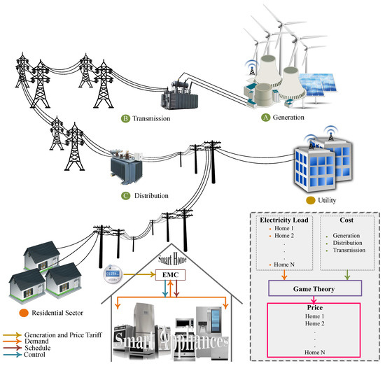
Under DR program different electricity tariffs (i.e., ToU, RTP, CPP, etc.) have been defined in order to reduce electricity demand during the on-peak hours. The DR strategy provides the incentive to shift the load from on-peak to off-peak hours. Where prices during the off-peak hours are low as compared to the on-peak hours. The prices during the on-peak hours increase as the demand of electricity increases and the excessive demand is fulfilled by costly energy generation units i.e., (fuel generators). The electricity per unit price is not only about the generation cost; however, there are also some other factors. The main factors that effect the electricity price signals are: generation cost, transmission cost and distribution cost [6] as described in Figure 1. The prices are highly influenced by the user demand and utility. Utility is known as service provider, it regulates the electricity rate seasonally (ToU and CPP), weekly, daily or hourly (variable peak price rebate or RTP).
Figure 1.
Proposed system model for GT pricing model and energy management scheduler.
In this paper, an enhanced ToU tariff based on GT (GTToU) is proposed for a residential sector. In this model, each user’ s per unit price of shoulder-peak and on-peak hour is calculated according to the electricity load profile and extra generation cost. Further, the proposed scheme is compared with that of day-ahead RTP. An overview of the proposed system model and information flow between the system components is provided in Figure 1. The electricity used by the end user passed through different processes. First, the generated energy is transmitted towards the distribution units through transmission lines. In the distributed unit, transformers stepping down the energy voltage to the level used by the consumer and distributed towards the end users through distribution lines. In this work, each home is considered as a smart home. A smart meter and an Energy Management Controller (EMC) are installed at each home. The smart meter acts as a gateway to exchange the information between the utility and a smart home. The EMC manages and controls the electricity load by scheduling the smart electrical appliances. A scheduler installed in the EMC schedules appliances according to constraint(s) defined by the optimization framework [40]. In this proposed work, utility asks for the user energy demand before the start of the day and it could be one hour before or 5 minutes before. The constraint (threshold level) will be set by the utility and scheduler according to the provided information. In our proposed work appliances are scheduled from on-peak to off-peak hours according to the provided electricity rates and demand through smart meter.
The utility has a price regulator that calculates each user’s shoulder-peak and on-peak price according to the consumed power. The utility also monitors the other costs (i.e., generation, transmission and distribution cost). However, in our scenario, we focus on the users’ power consumption. The price regulator calculates the price using GT and updates the users through the smart meter. Moreover, the user manages the load during the shoulder-peak and on-peak hours through scheduling. Whereas a meta-heuristic-based scheduler is embedded in EMC. In addition, we consider two meta-heuristic algorithms, SSA and RFA.
3.1. Formulation of GTToU
Due to the high demand of electricity during some specific hours, generation increases and has impact on electricity price and user’ s electricity bill. In this section, a mathematical model is formulated to enhance the ToU electricity price signals. In ToU rate, a day is broken up into three blocks: on-peak, shoulder-peak and off-peak. Prices during the on-peak and shoulder-peak hours are high due to high demand and generation units. It is worth mentioning here that each customer is charged the same price even if any of them shifts load towards off-peak hours. In this proposed price rate, each user’s per unit price is calculated during the shoulder-peak and on-peak hours according to the generation of extra energy and users’ consumed electricity. Further, in this section, we will discuss the constrained-based scheduling problem. The focus of the proposed work is cost minimization. Besides, the load shifting from on-peak and shoulder-peak hours to off-peak hours is also done.
3.1.1. Modified ToU Tariff
The modified ToU tariff is based on the extra generation cost and the load demand of user’s during the specific hours. The changes per hour units are made for shoulder-peak and on-peak hours. The formal representation of modified ToU price signal () is given as (1):
where represents the off-peak hours. Utilities define the price rate according to the demand, where electricity prices are high during the periods of high power demand (on-peak hours) and lower during the periods of low power demand (off-peak hours) [41]. off-peak hours are usually when homes and offices use less electricity.
In this scenario, we consider on-peak and Shoulder peak as on-peak hours. The h denotes the N number of homes () in a specific area. The value of ℑ depends on extra cost (ß%) rather than the off-peak price, the value of ß% depends upon the extra generated energy. The increasing amount of generation will increase the ß percentage of user per unit charge. The ß% amount will be distributed among all the users within a specific time interval according to their consumed electric energy.
3.1.2. Electricity Cost Minimization
DSM strategy, load shifting is adopted to reduce the electricity cost. EMC is used for home load management and appliances scheduling. However, this load shifting may results in undesirable rebound peaks because every consumer tries to reduce the electricity bill. To tackle with the rebound peak issue, we have proposed a constraint-based electricity cost minimization function. Here, electricity load is shifted from shoulder-peak and on-peak hours towards off-peak hours according to given constraint in Equation (3). In this equation, a threshold level according to aggregate load of all connected homes is defined for the on-peak, shoulder-peak and off-peak hours. The scheduler installed in energy management controller schedules the load according to the limits of power demand. It also prevents the rebound peak. The objective function of electricity cost minimization is mathematically written as:
Subject to the constraint:
where denotes standard deviation; is the total aggregated load of N homes. Appliances will be scheduled according to the constraint defined in Equation (3). In this equation, load limits are defined for the on-peak and off-peak hours. This threshold avoids the load to increase from a specific limit which helps in avoiding the rebound peak. The electricity load of an individual home is calculated as:
where represents the On and Off status of an appliance. The total electricity cost is calculated as:
The Equation (9) is formulated to calculate the .
where is the list of electricity price signal.
4. Proposed Methodology
4.1. GT Based Price Model
In this section, the proposed GTToU tariff is briefly discussed. In this work, the ToU price signals are enhanced using cooperative GT. In cooperative game, players cooperate to form some coalitions to distribute the profit according to the contribution (pay-off). The player with maximum contribution can obtain more profit. Every participant in coalition wants maximum profit [42]. In cooperative GT, Shapley value, a solution concept is proposed in [43]. In this work, the concept of Shapley value is used for fair distribution of extra generation cost among the N homes in a coalitional game . Fair in the sense, the home with maximum load has been charged more as compared to the customer who shifted the peak load. The extra generation cost that will be added in the home h electricity bill is calculated as [44]:
The Shapely value is expected electricity cost (pay-off or marginal distribution) of home h. Where ℵ is a set of N homes and is the function that maps subsets of ℵ to the real numbers ℜ (i.e., →ℜ). The represents the number of member in a coalition S and (=N) is the total number of homes. For coalition S, describes the total expected sum of marginal distribution that a member of S can obtain. In Equation (10), numerator is equal to the number of permutations of S whereas denominator is the total number of permutation [42]. Permutation is used to find out all the possibilities in which coalition can formed, for N homes it is calculated as . The complexity of electricity bill calculation procedure is .
4.2. SSA Based Scheduling Model
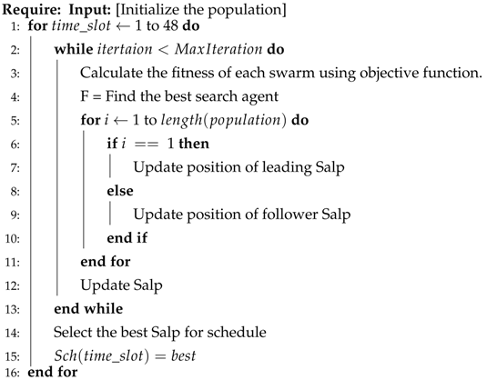
To optimally schedule the home appliances, SSA home appliances scheduling mechanism is proposed in this work as given in Algorithm 1. SSA behaviour is adopted from the Salps swarm navigating and foraging behaviour in oceans. Salp belongs to the Salpidae’ s family. The main motivation to adopt this technique for optimization is their swarming behaviour where all Salps move and forage food together [45]. This behaviour helps the Salp to explore and exploit the search space.
In this EMC, each salp is considered as an appliance. Where the target is to find the best swarm, i.e., a group of appliances. The salps’ swarm move together and find an optimal solution to survive. In our case, a group of appliances will have to find the best optimal point during a time-interval. Where, its target is to consume a moderate level of electricity so that neither it creates peak nor increases the price.
| Algorithm 1 Pseudocode of Salp swarm optimization |
 |
SAA
There is a chain of Salp swarm. This swarm is then divided into leaders and followers. A Salp leading a chain is said to be a leader Salp and others are follower Salps. The leader Salp guides the follower Salp. An n-dimensional search space is considered. n indicates the number of variables of a given optimization problem. X is a two-dimensional matrix used to denote the positions of Salps. F is a food source assumed in the search space. A Salp target inside the search space is F.
Following equation is used to update the leader position [45].
j is a dimension of a search space. is a position of leader Salp in a jth dimensional search space. is considered as a food source in jth dimensional search space. Where and are the upper and lower bounds of search space with dimension j. , and are random numbers.
The leader Salp position depends on the food source. is a coefficient. balance the exploration and exploitation. It is a very important parameter for Salp algorithm.
and are random numbers. The value of and is 0.5. and decides whether the next step should be towards positive or negative infinity.
Newton’s law of motion is used to update the position of follower Salps. Equation (13) is used for this purpose:
where indicates the position of follower Salp in search space of dimension j. t shows the iteration, represents the initial speed. Where and . The above equation can be expressed as:
4.3. RFA Based Scheduling Model
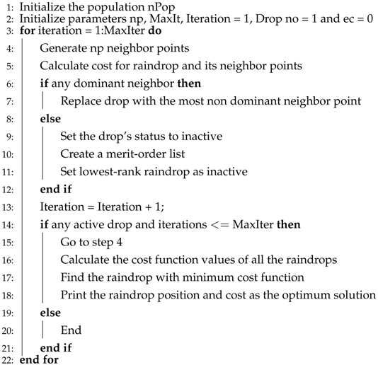
To optimally schedule the home appliances, RFA is proposed in this work. RFA mimics the behavior of rain drops. In EMC, each drop of rain is considered as an appliance. The drops of the water are collected in the deepest valley (local search) and then reach the global optimal solution (i.e., sea level).
4.3.1. RFA
In the RFA, the particles move like gradient descent and hill climbing. The pseudocode of the proposed work is given in Algorithm 2. RFA optimization starts with initialization of population and parameters used. The terms used in the proposed algorithm are: raindrop, neighborhood, neighbor point, active drop, inactive drop, explosion process, raindrops rank and merit order list. These terms are described below.
| Algorithm 2 Pseudocode of Rain-fall optimization |
 |
4.3.2. Raindrop
A single particle of a population is said to be a raindrop. It is a vector used to store the variables involved in optimization problem. It is used to satisfy the constraints of the optimization problem. m represents the size of the population, i is used to show the drop numbers. It is defined in Equation (15) [46].
where n is used to represent the variables used in optimization problem, shows the kth variable used in optimization problem. is the ith drop number. The constraint used is given in Equation (16) [46].
where U is used to show uniform distribution function. Upper and lower limits are represented as and .
4.3.3. Neighborhood
Neighborhood is the domain with radius r around raindrop in N-dimensional search space. It changes with the change of raindrop value.
4.3.4. Neighbor Point
In optimization, a random generation of a point is said to be a neighbor point. shows the neighbor point j of raindrop i. The formula for is given below in Equations (17) and (18) [46]:
whereas, , and , and r shows real vector, is the initial neighborhood size and np represents the neighborhood points.
4.3.5. Dominant Drop
The point performs well in neighborhood is said to be dominant. It reaches a optimum value of given objective problem. Dominant drop is represented as . F shows the function required to solve objective problem. Following formulas are used to find the value of raindrop and its neighbor point ().
4.3.6. Active Drop
The variable having a dominant neighbor is said to be active drop.
4.3.7. Inactive Drop
The variable having no dominant neighbor is said to be inactive drop.
4.3.8. Explosion Process
The explosion process is done when the drop is inactive, i.e., it has no dominant neighbor during optimization or there are not sufficient neighbors. This process is done to take rain drop out of this situation. The explosion process runs for Ne times. (np(ex)) is used to verify the neighbors in explosion process as Equation (20) in [46].
where neighbor points are represented as np, explosion base is shown as eb and the explosion counter is given as ec.
4.3.9. Raindrops Rank
There is a merit list in which different ranks are given to all raindrops. The ranks of raindrops are calculated as Equations (21)–(23) in [46].
where and are weighting co-efficients. The value of and is 0.5. and shows the change in value of objective function for raindrops at iteration t. shows the rank of rain drop at iteration t.
4.3.10. Merit Order List
A merit list is used to save the ranks of raindrops in ascending order. A raindrop from merit list is removed and considered in optimization problem. At first iteration, the raindrops are generated randomly. After generation of raindrop, a neighborhood is assigned to each raindrop and the neighbor points are also generated randomly according to the constraints of objective function. Some constraints are discussed below for assigning neighbor points using Equations (24) and (25) [46]:
The cost is calculated for each rain drop and its neighbors. All values of neighborhood are compared with value of raindrop to find out the most dominating neighbor point.
5. Simulation Results and Discussion
5.1. Experiment Configuration
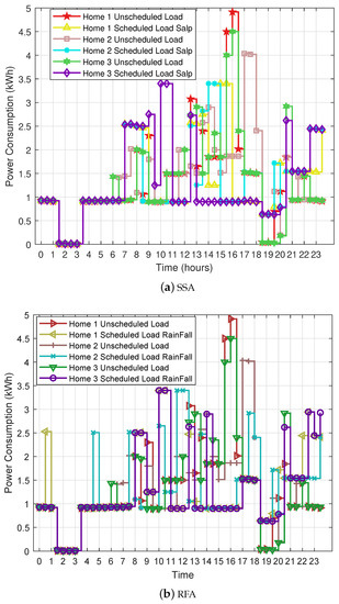
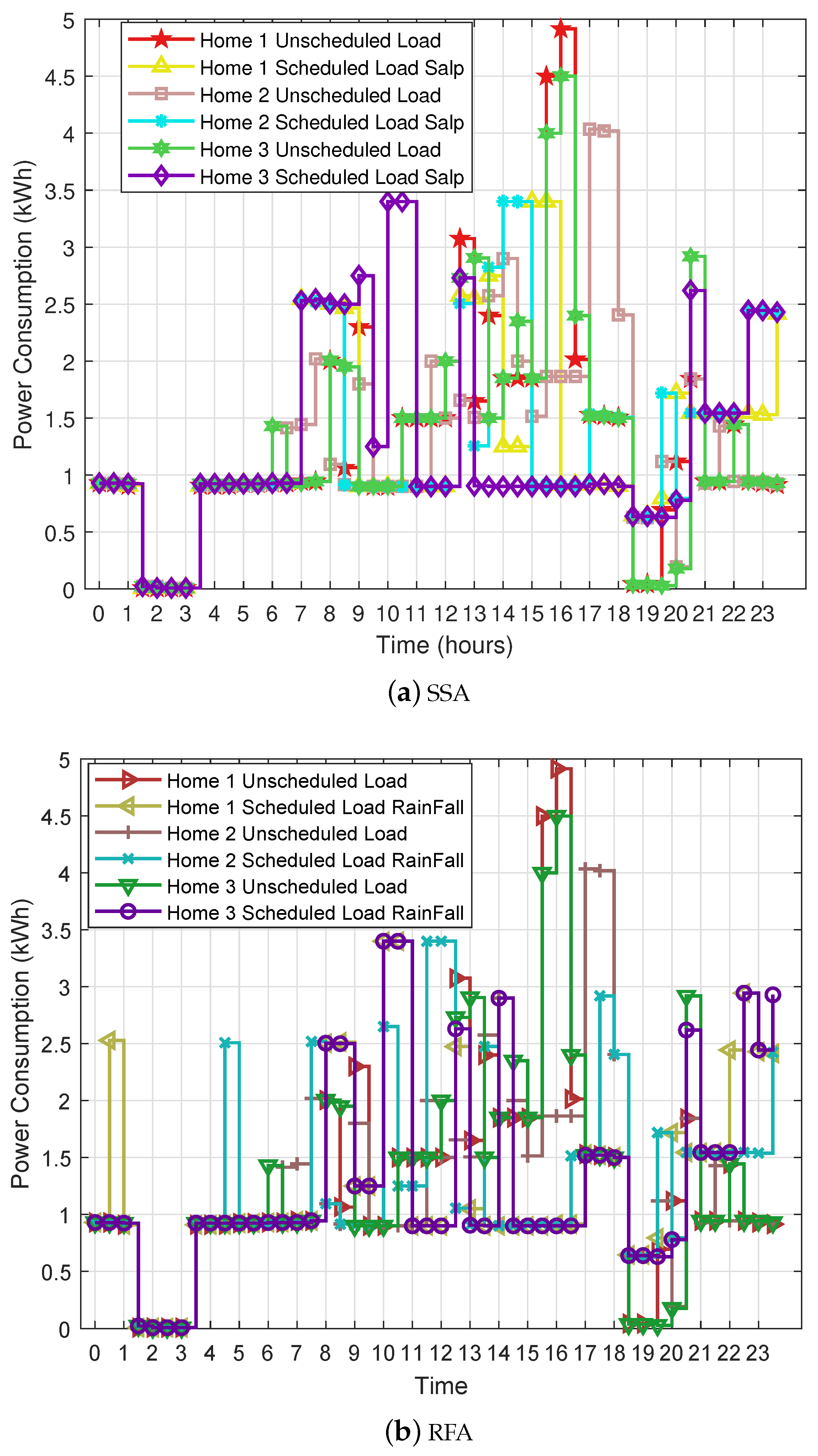
Simulations are performed to investigate the impact of GTToU and compared with Flat Rate (FR) and ToU (seasonal fixed) price signal on the user’s electricity bill. The FR is considered as a baseline electricity rate in [47]. As discussed earlier, dynamic and time-based electricity rates determine on the basis of generation cost and consumed energy. However, generation cost is somehow confidential. So, for this experimental study, we assume an increase in the generation where rates of ToU price are high. The FR and ToU tariff for this experimental study is taken from [5]. The ToU tariff is given in Figure 2. The FR price for each hour remains fix and it is per kWh up to 1000 kWh and for more than 1000 kWh. In order to find the difference in the total cost and per unit price, three homes are considered with the same number of appliances and the same load demand. However, appliances operational time varies according to the customer life style as shown in Figure 3.
Figure 2.
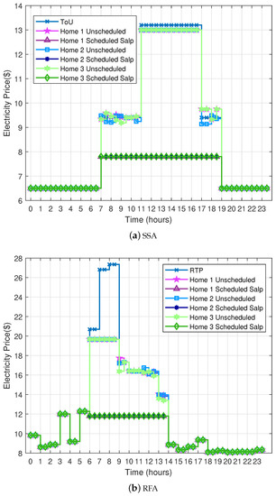
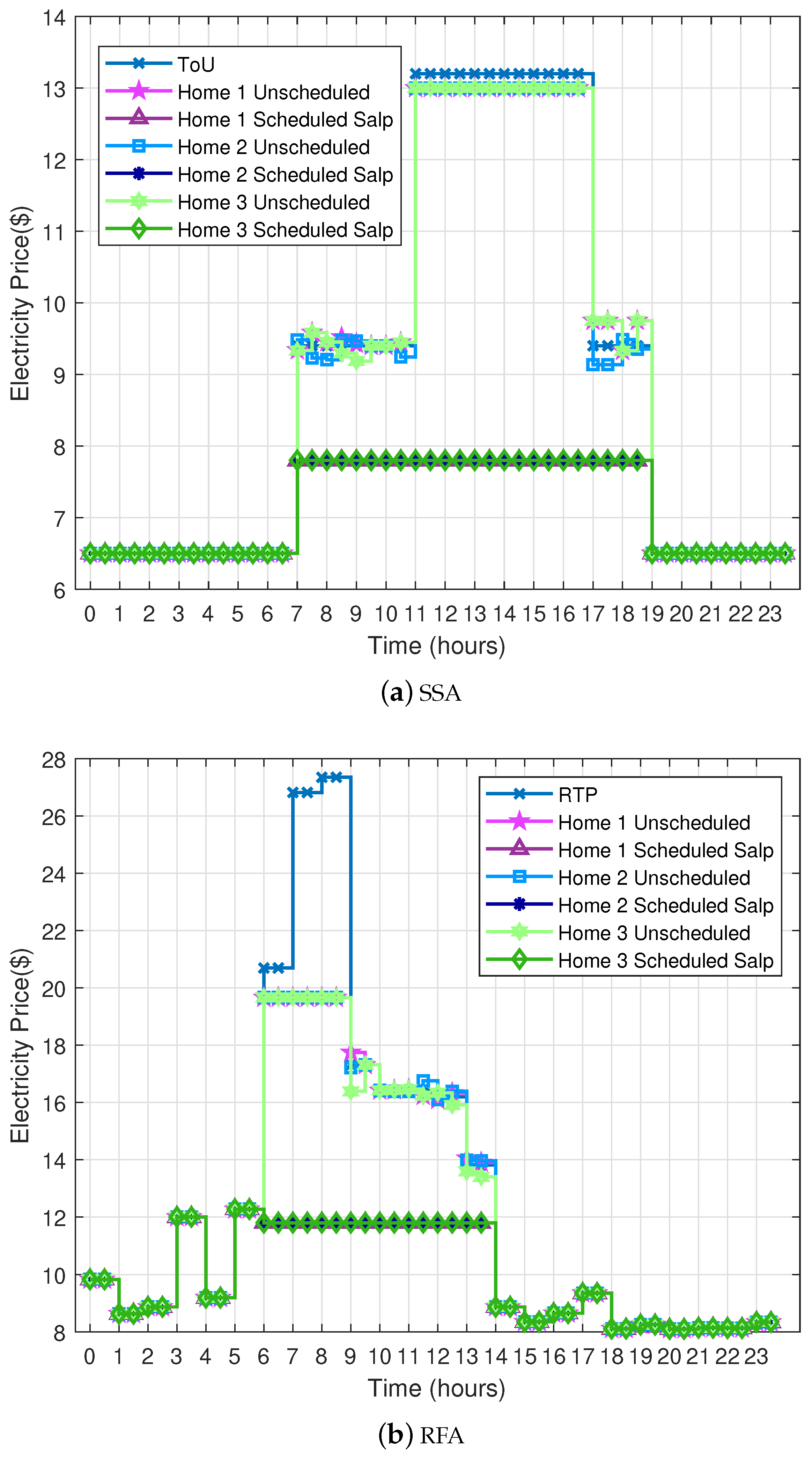
ToU price regulated by PG&E and price according to the proposed scheme.
Figure 3.
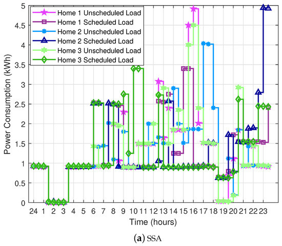
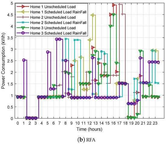
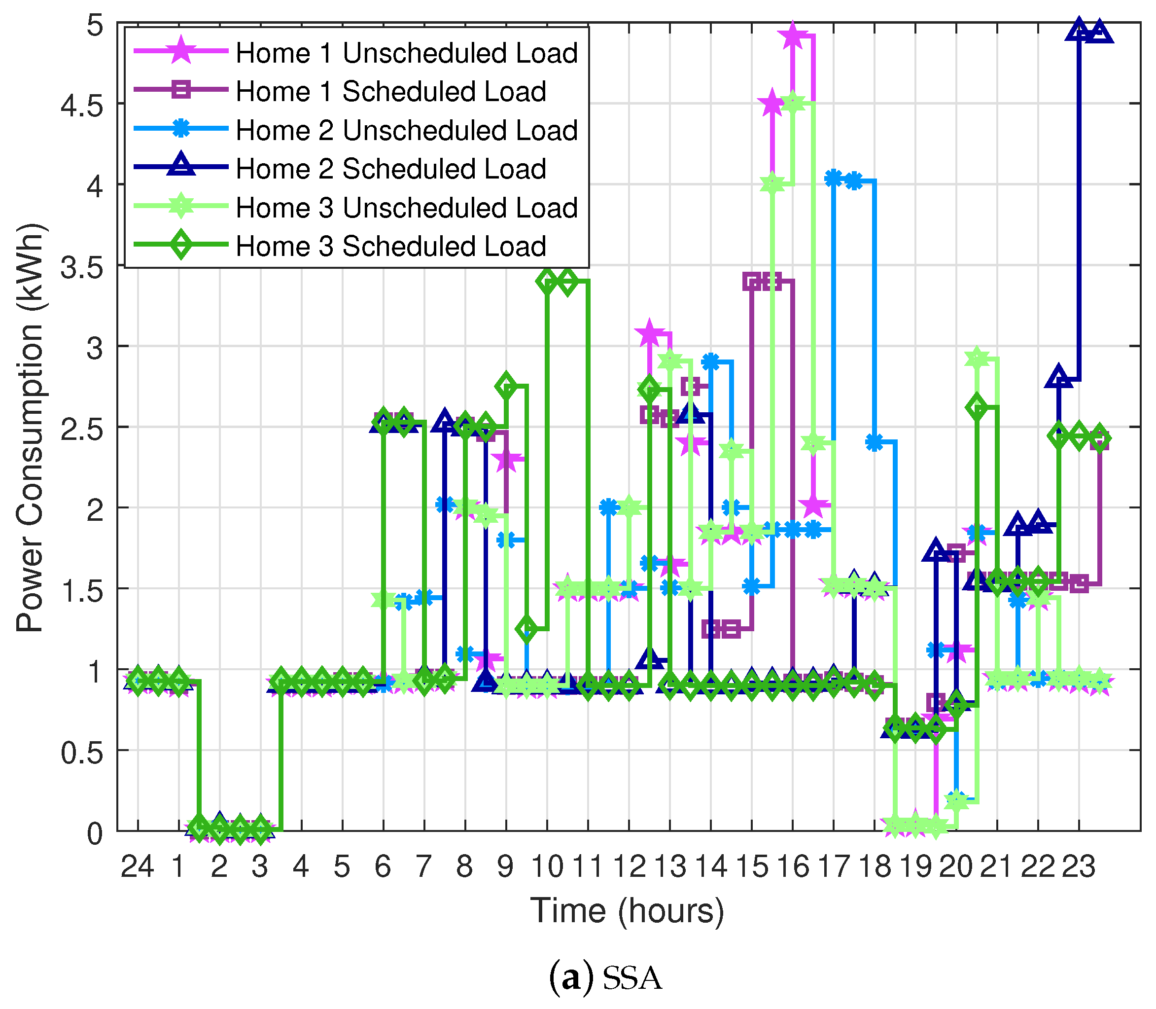
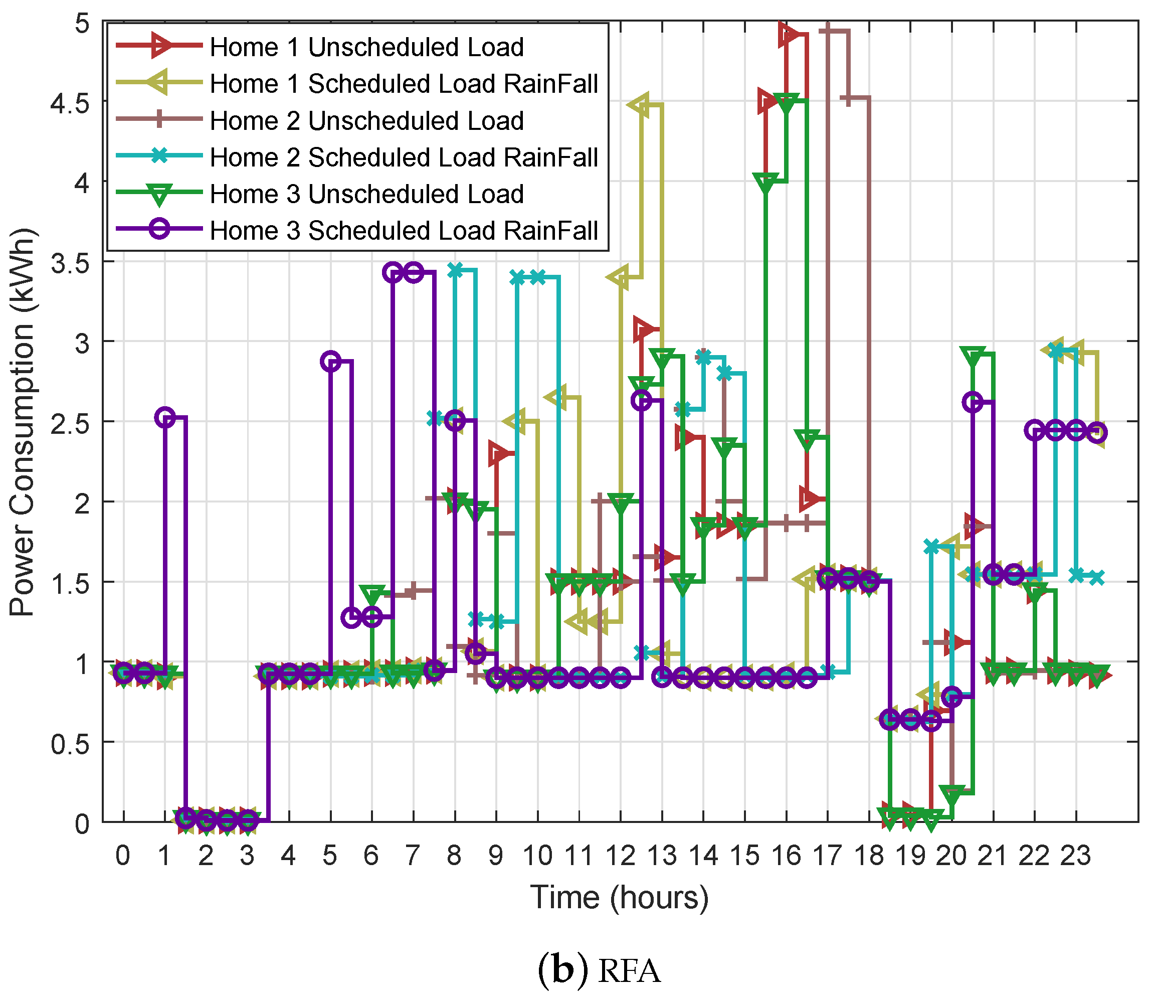
Load profiles of three homes before and after scheduling with ToU and GTToU.
The electricity bill can be further reduced after scheduling the electric appliances. Further experiments are carried out to study the impact of scheduling using two meta-heuristic optimization algorithms: SSA and RFA. We also investigated the impact of proposed pricing technique after load shifting through scheduling.
Three smart homes are considered for scheduling where each home has 12 appliances. For fair comparison of three homes’ electricity bill, we have considered the same energy demand by each user. The detailed description of each appliance is given in Table 1. The selected appliances have three groups: schedulable interruptible, schedulable non-interruptible and non-schedulable appliances. Different time slots can be allocated for interruptible appliances, whereas non-interruptible appliances cannot be interrupted during the working cycle (e.g., washing machine and cloth dryer). Moreover, dishwasher will always start working after the oven. There could be a gap between oven and dishwasher. However, this gap is not acceptable in case of cloth dryer and washing machine.
Table 1.
Detail description of appliances used in simulations.
5.2. Experimental Results for GTToU
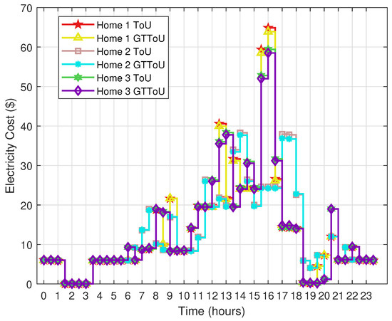
The difference in electricity cost for FR, GT-based ToU price (GTToU) and ToU without scheduling can be envisioned in Figure 4. In this figure, the electricity price of each user changes according to the consumed energy during the shoulder-peak and on-peak hours.
Figure 4.
Electricity bill of three users before scheduling with ToU and GTToU.
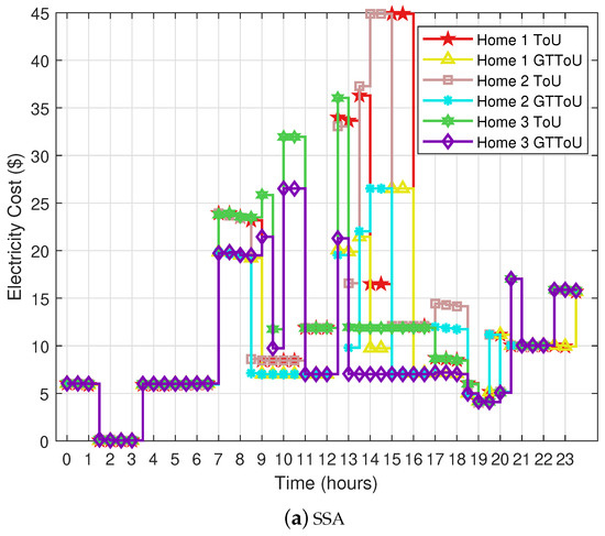
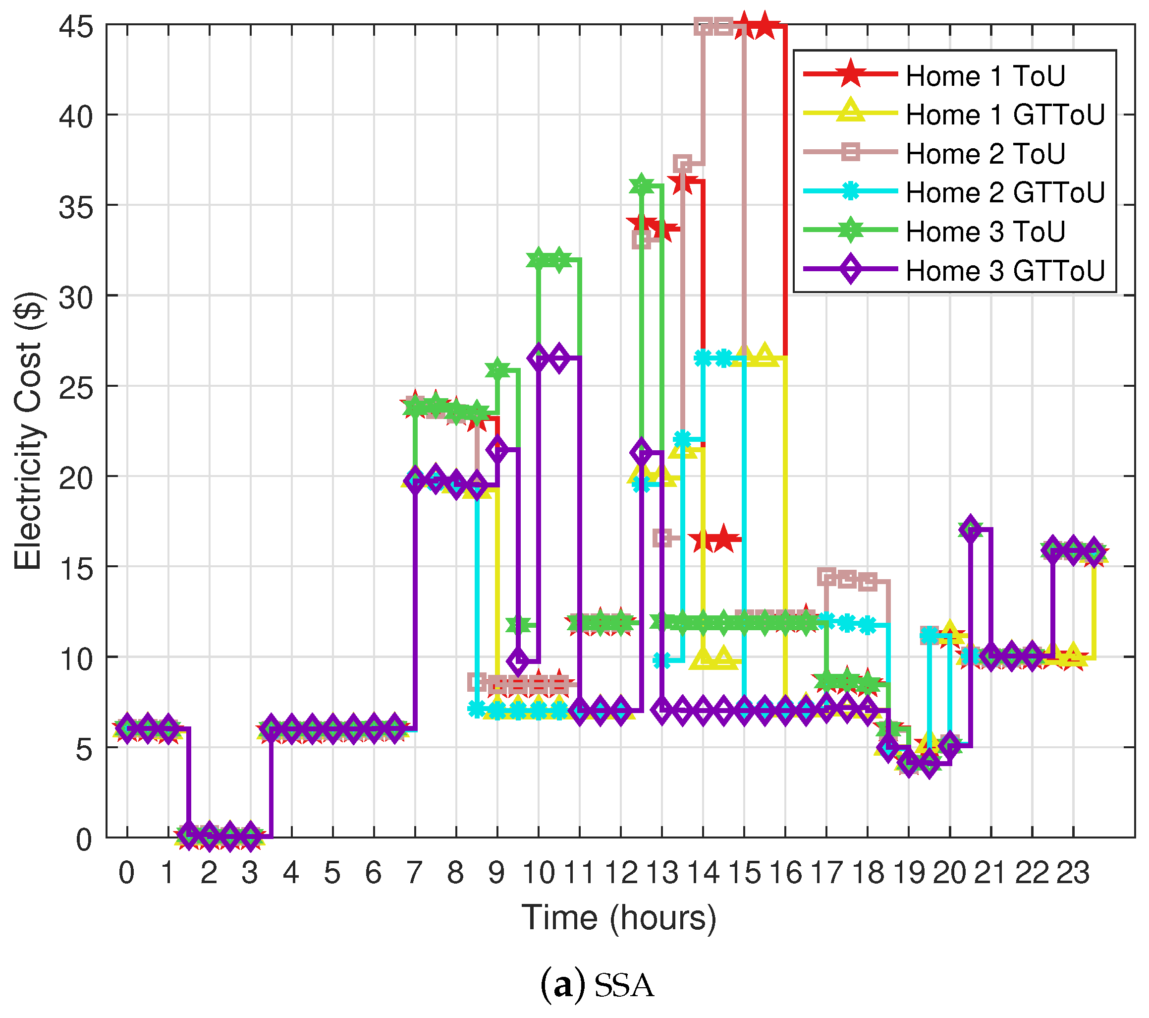
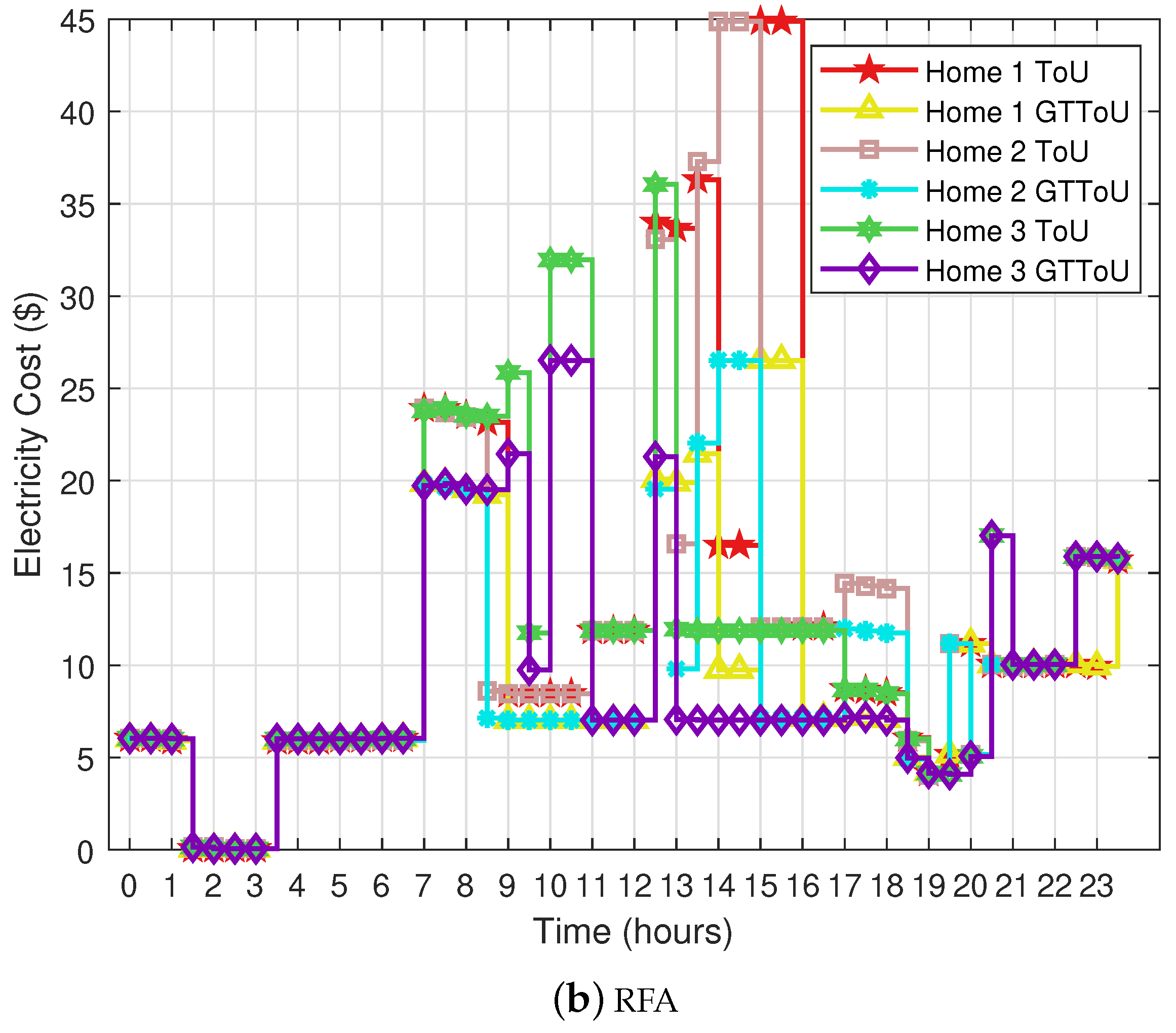
A slightly different behaviour in scheduled load is observed with the RFA, as shown in Figure 2b. At the 7 p.m. point, the unscheduled power consumption of Home 2 is less than Home 1 and 3 and the price is also minimized for this particular slot (see Figure 2 and Figure 3) which shows reduction in electricity cost as shown in Figure 5. Moreover, the Figure 5a,b show that the load at 6:30 p.m. is the same for Home 3.
Figure 5.
Effect of scheduling on electricity cost for ToU and GTToU.
The price during the off-peak hours remain same. From simulation results, it is analyzed that using FR, a user has to pay 483.767¢ for 62.870 kW for one day load. Which is higher than the scheduled load by RFA. While comparing GTToU with ToU approximately, 1% decrement is observed in electricity bill using GTToU. However, this difference is increased after scheduling as described in Table 2. With Salp scheduler, the difference between between scheduled and unscheduled cost for the three homes is calculated as 6%, 4% and 13%. Whereas RFA scheduler outperformed by reducing 14%, 5% and 12% electricity cost. This shows that the price is reduced after shifting the peak load from on-peak hours towards the off-peak hours. Moreover, the electricity cost per hour is decreased for each home using the GT model. The percentage difference of cost between scheduled and unscheduled homes using GTToU is 28% for Home 1, 25% for Home 2 and 29% for Home 3 for SSA. Whereas for RFA, the difference is 32%, 29% and 31% of targeted homes.
Table 2.
Electricity cost (¢) before and after scheduling with ToU and GTToU.
If we compare ToU and GTToU electricity cost after scheduling, it is observed that electricity cost decreases after calculating the price using GTToU up-to 21%, 26% and 23% for Home 1, Home 2 and Home 3, respectively for RFA. Similar behavior is observed for SSA, where 24%, 23% and 19% decrease in cost for GTToU is observed for Home 1, Home 2 and Home 3, respectively. Table 2 shows that each home electricity cost is different although each home has the same load. This shows that the home with the maximum load during on-peak hour has a high electricity bill. In summary, the proposed pricing scheme GTToU outperformed as compare to ToU rate after scheduling.
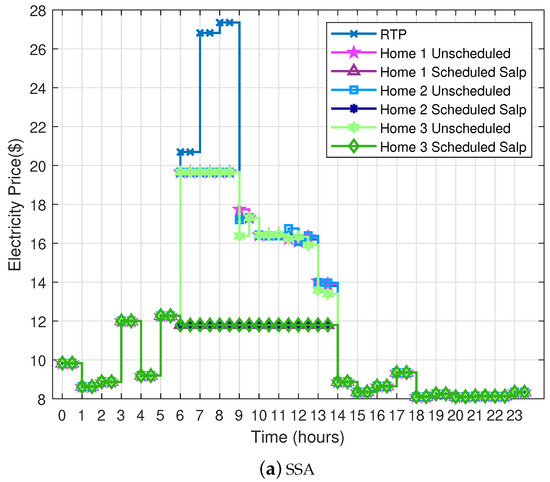
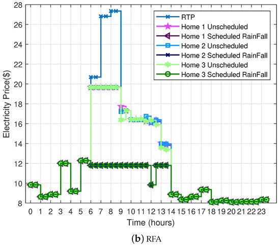
The impact of scheduled load on price is given in Figure 2. This figure depicts that the electricity price changes according to the user load profile given in Figure 3. As shown in Figure 3a for Salp algorithm, at 6 p.m. (shoulder-peak hour) load of Home 1 and Home 3 is higher than the Home 2 which reflects the price rate (see Figure 2a) whereas the cost of Home 1 and 3 is higher than the Home 2. After scheduling, a remarkable difference is observed in electricity cost and PAR as given in Table 2. The overall percentage difference is 4% in cost after scheduling with GTToU. Where the PAR difference for scheduled and unscheduled homes is 52% for Home 1, 29% for Home 2 and 43% for Home 3. This reduction in PAR shows that proposed constraint-based cost minimization function avoid the peak rebounding. Moreover, from Figure 3 it can be observed that the maximum unscheduled power load is 5 kWh; however, after scheduling maximum peak load is 3.5 kWh.
5.3. Experimental Results for Day-Ahead RTP
The RTP price can be defined as a week-ahead, day-ahead and an hour-ahead. The week-ahead and day-ahead pricing schemes are determined on the basis of previous electricity demand. RTP hourly pricing scheme is defined as the projection of incremental demand and generation cost per day. It is easy to schedule the electrical appliances for week-ahead and a day-ahead pricing schemes. However, scheduling of appliances for an hour-ahead pricing scheme is quite challenging. The price during on-peak and off-peak hours varies, so it is difficult to schedule the appliances for an hour-ahead pricing strategy. Load forecasting can be used to tackle the aforementioned problem.
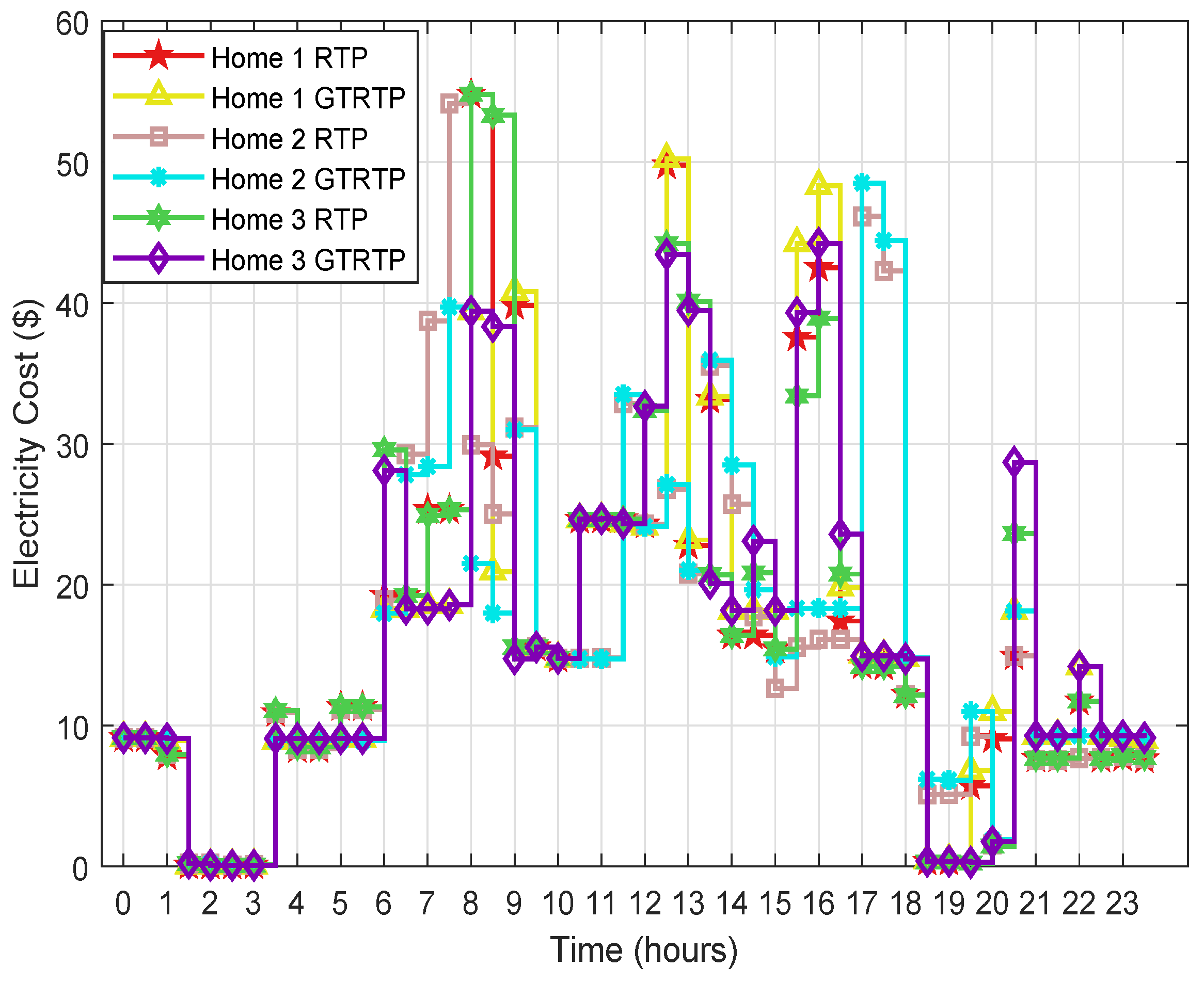
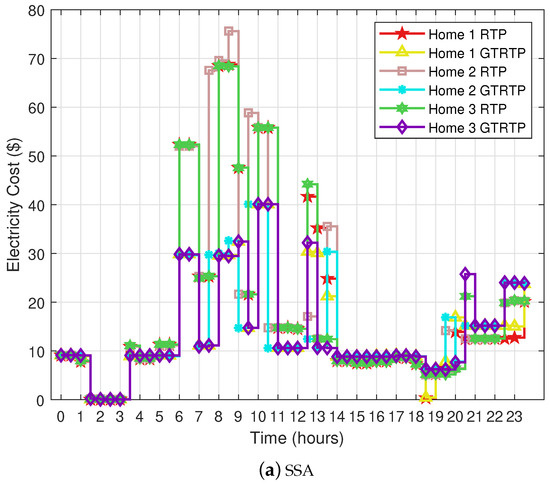
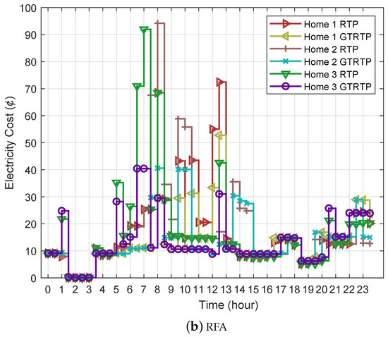
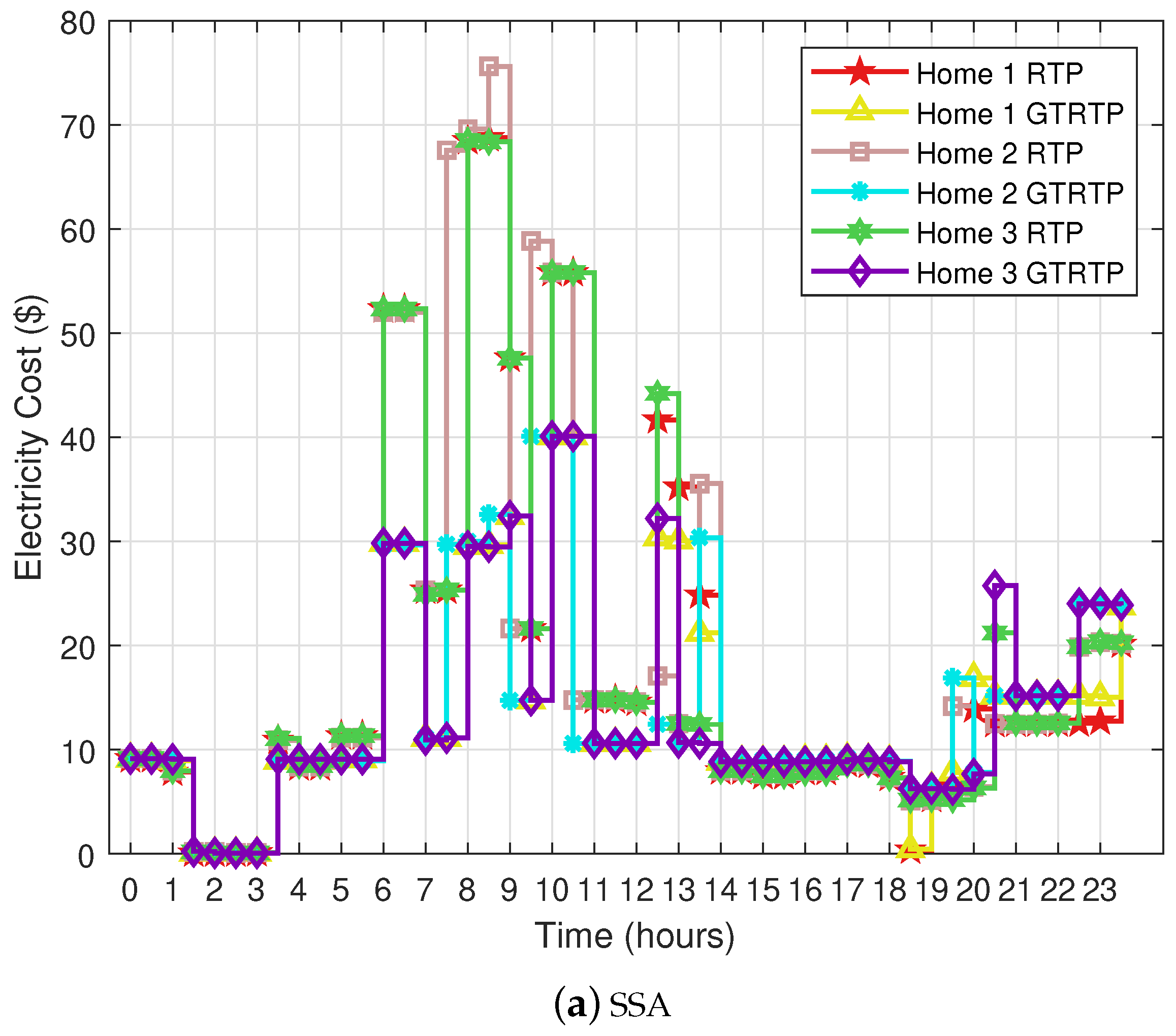
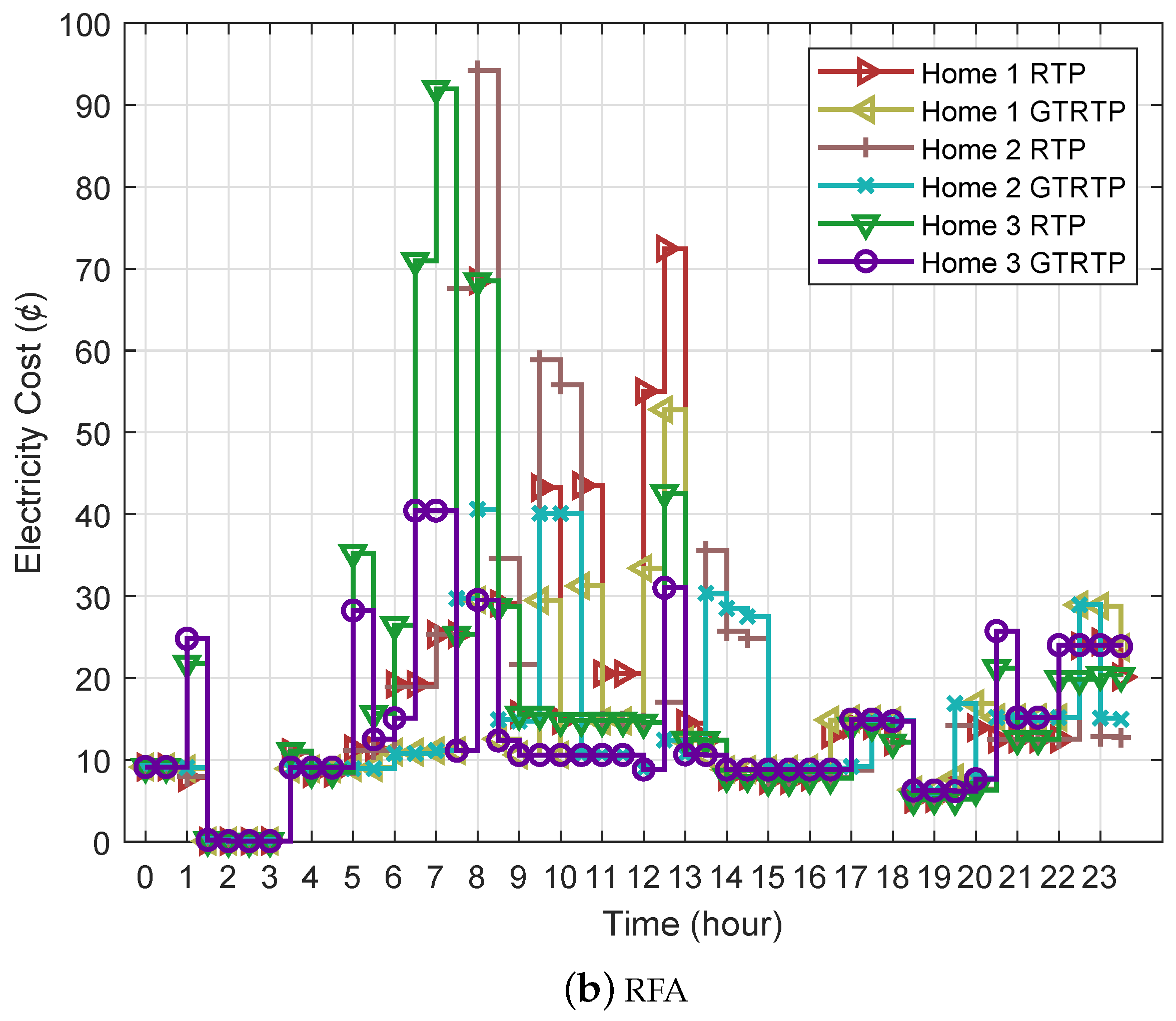
The proposed SSA-based scheduling scheme is tested for day-ahead RTP signals. The results are given in Figure 6, it depicts that the load is increased during the on-peak hours which affects the electricity cost. A minor difference (i.e., 1%) is observed between RTP and GTRTP price as shown in Table 3. However, the cost is increased with both schedulers. 13% cost is increased for Home 2 with Salp scheduler and 7% is increased with RFA for the same home. However, it is observed that the cost and price decreased after scheduling with GTRTP. The total difference in cost between the scheduled and unscheduled cost using Salp is 14%, 14% and 15% for Home 1, 2 and 3, whereas the difference is 16%, 15% and 16% with RFA. The results further confirmed that the RFA outperformed. The PAR value decreases up to 52% with Salp and 17% for RFA. In Figure 6, at 11:30 a.m., the energy consumption of Home 2 is higher than the Home 1 and 3.
Figure 6.
Load profiles of three homes before and after scheduling with RTP and GTRTP.
Table 3.
Electricity cost before and after scheduling for ToU and GTToU.
It can be envisioned from Figure 7 and Figure 8 that the electricity cost is not high during some specific hours. After scheduling the cost varies accordingly. Figure 9 shows that the price during on-peak hours is reduced due to the shifting of load. To avoid the peak formation, scheduling is done. The PAR value decreases up to 52% with Salp and 17% for RFA. In Figure 6, at 11:30 a.m., the energy consumption of Home 2 is higher than the Home 1 and 3. Further, Figure 3 and Figure 6 show the peak load and cost during on-peak and off-peak hours. The RFA efficiently dealt with the distribution of load during on-peak hours. Despite this, there is a minor difference between SSA and RFA. As shown in Figure 6a,b, RFA avoids peak formation and keeps the load on the average level. A Salp algorithm somewhere exceeds the average level (Figure 6a).
Figure 7.
Electricity bill of three user before scheduling with RTP and GTRTP.
Figure 8.
Effect of scheduling on electricity cost with RTP and GTRTP.
Figure 9.
RTP tariff and electricity price of all three homes according to the proposed scheme.
The results of ToU and day-ahead RTP tariff policies show that ToU is more convenient. In ToU tariff policy, the consumers have to pay less than the RTP users. Moreover, the proposed scheme efficiently reduced the electricity bill. Before scheduling, the difference between the electricity bill of ToU and GTToU is less. However, GTToU is effective after scheduling. Moreover, the simulation results depict that RFA effectively explores and exploits the search space.
The day-ahead RTP and ToU pricing schemes are efficient for scheduling the load profiles of electricity. The RTP has been defined for week-ahead, day-ahead and hour-ahead pricing schemes. The week-ahead and day-ahead pricing schemes are defined on the bases of previous electricity demand. The pricing scheme for an hour is defined for RTP hour-ahead price. It depends on the prediction of incremental demand and generation cost per day. It is easy to schedule electrical appliances using week-ahead and day-ahead pricing schemes. However, for an hour-ahead pricing scheme, it is difficult to schedule the appliances as the price per hour is different. Load forecasting is one of the solutions to solve the aforementioned issues. For this purpose, simulations are done for the load forecasting to deal with hourly ahead RTP signal using ensemble classifiers.
5.4. Experimental Results for Ensemble Regression
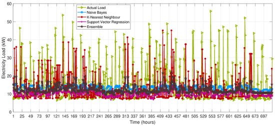
In order to study the impact of ensemble classifiers on load prediction, the weather and load data is taken from [48]. The datasets available in [49] contain the weather and energy consumption record of different homes. From this available records, we analyze and predict the Home A power load. This data contains the each mints load and weather detail.
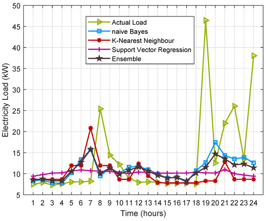
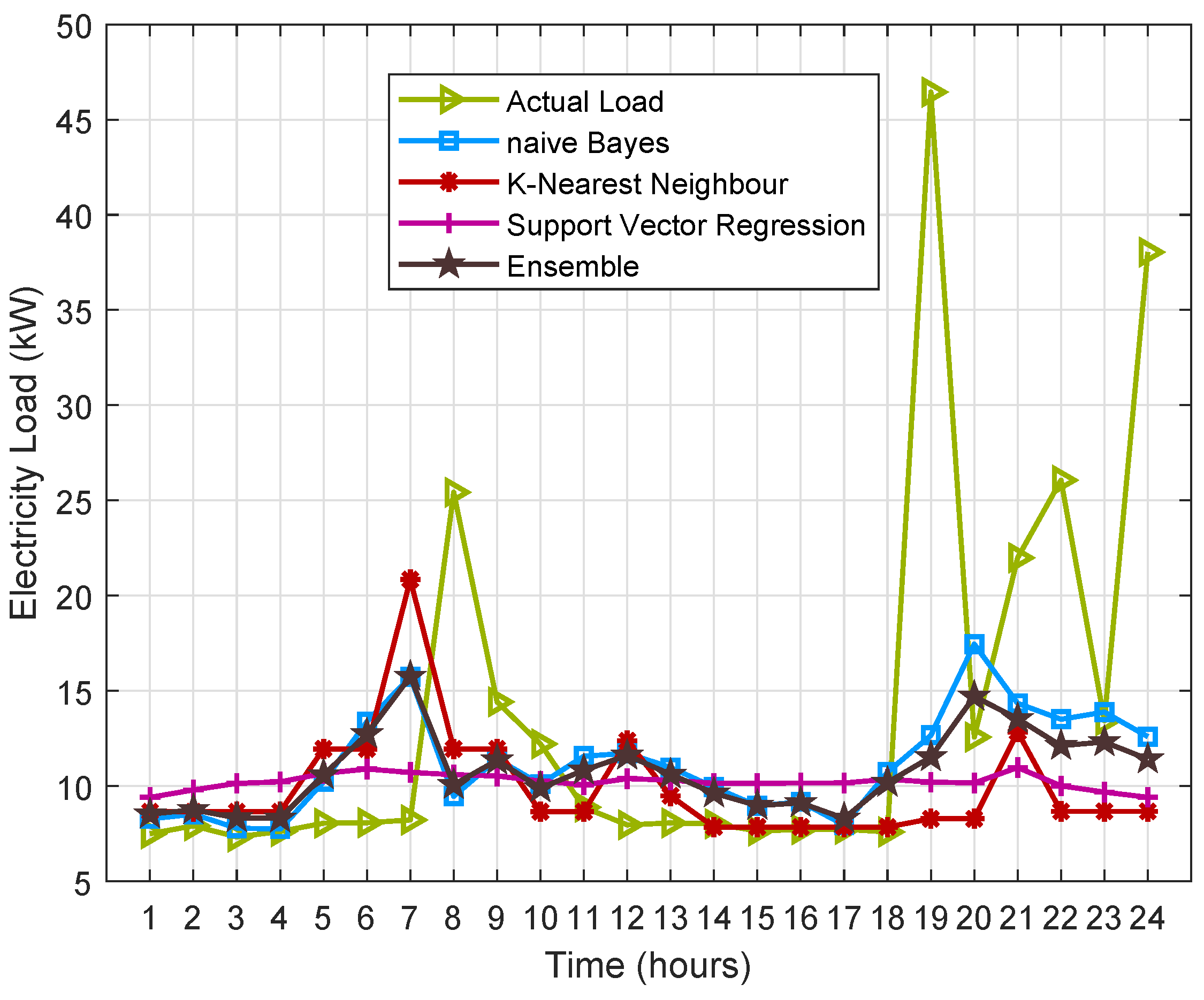
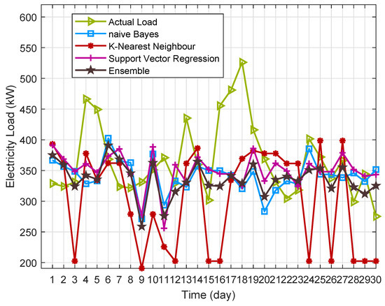
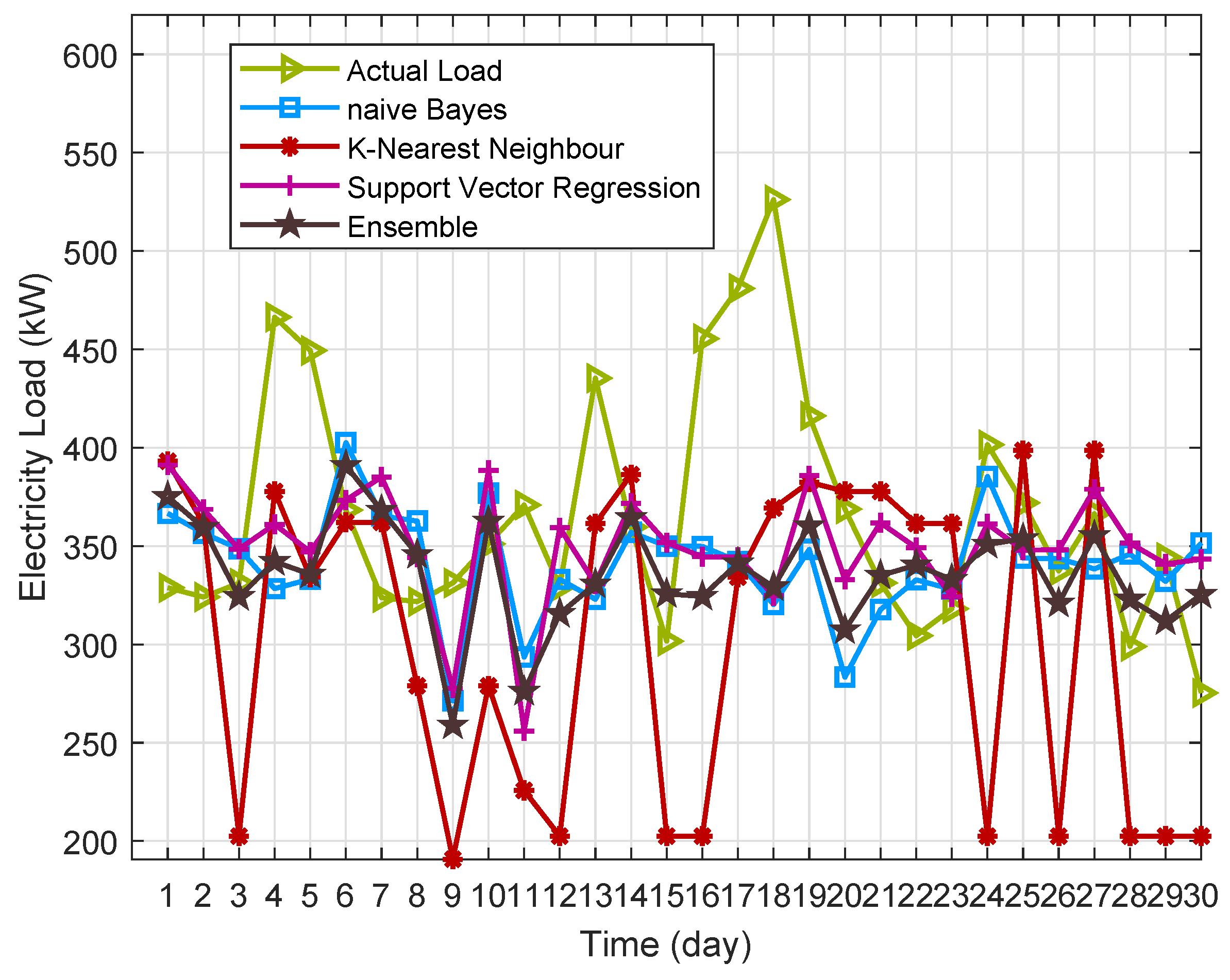
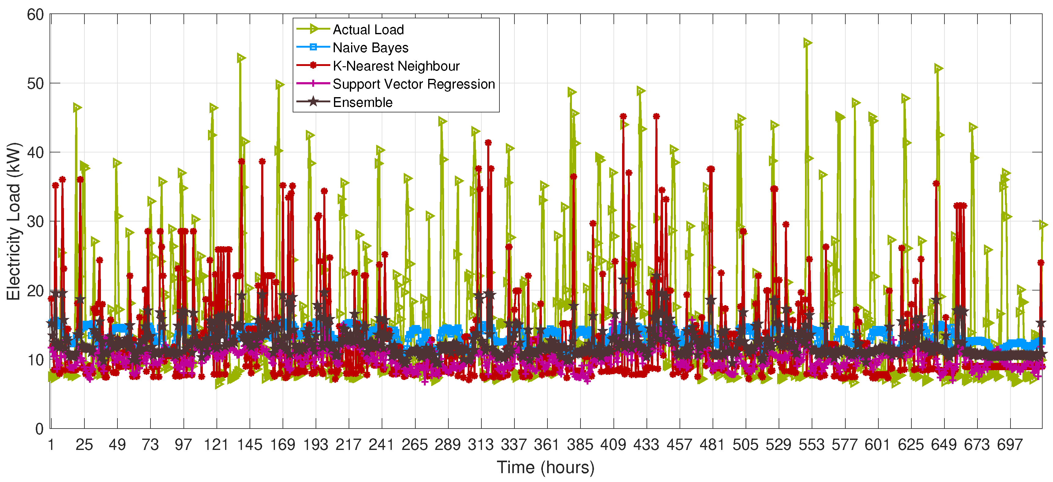
In the proposed work, the data of summer season is considered. So the data for June, July, August and September is taken. Regression model is used to train the data of June–August. Whereas the testing is performed on the data of September. The prediction of load depends on the conditions of the weather. To analyze the behaviour of regression model, different load patterns are studied as given in Figure 10, Figure 11 and Figure 12. These figures show the users behaviour for an hour, day and month.
Figure 10.
Predicted load of a day.
Figure 11.
Predicted load of a month.
Figure 12.
Per-hour predicted load of a month.
Figure 10 shows that the load profile of users is stochastic. The load demand is high in morning and evening. The electricity consumption also depends on the working hours. For one day prediction, only the first day of each month is taken for the purpose of training and testing. The Figure 10 shows that the K-nearest neighbour prediction is different from the actual data.
The user electricity consumption is given in Figure 11. Where electricity load profile shows a different behaviour for each day. From this, we analyze that the demand for a day and hour changes as given in Figure 12. Moreover, the minimum error is shown by Naive Bayes. However, its trend is different from the actual behaviour. From this trend, scheduler can estimate the on-peak and off-peak hours.
6. Conclusions
In this study, the coalition-based GT model is proposed to formulate the pricing scheme model. Dynamic DR price models are used to charge the electricity cost per unit. The main purpose of the proposed work is to shift the load from on-peak hours to off-peak hours. Furthermore, some incentives are also defined for users. However, a per unit cost is same for all users. There is a pay-off incentive for the users who have shifted the load from on-peak to off-peak hours. The purpose of the proposed model is to charge the per unit price according to the consumed energy and the extra generation cost. The shappley value distributes the extra generation cost among each user according to the electricity load profile. The cost is directly proportional to the load peak during on-peak hours. Moreover, SSA and RFA are used to automate home appliances. Experimental results show 50% reduction in PAR and 32% in cost with RFA using GTToU. This shows the effectiveness of RFA. A remarkable difference between schedule load price for ToU and the proposed technique is observed. However, this difference is minor for unscheduled ToU and GTToU electricity bill. The proposed scheme is further compared with day-ahead RTP. Simulation results show that the proposed GTToU price model is more cost effective as compared to day-ahead RTP. Moreover, electricity load is predicted using ensemble classifier for hourly-ahead RTP rates. Simulation results show that ensemble regression model outperformed the single regression model. In this work, we have studied ensemble classifiers impact on the load forecasting technique. In the future, we will enhance the techniques for load prediction.
Author Contributions
A.K., N.J. and M.I. proposed, implemented and wrote heuristic schemes. A.M., T.S. and A.R. wrote rest of the paper. All authors together organized and refined the paper.
Funding
This research received no external funding
Conflicts of Interest
The authors declare no conflict of interest
Nomenclature
| Symbols | Description | Symbols | Description |
| C/I | Curtailable/Interruptible | Total aggregated load of N homes | |
| CPP | Critical Peak Pricing | Constant value | |
| CPR | Critical Peak Rebate | Total electricity cost | |
| DR | Demand Response | ON and OFF status of appliance d | |
| EMC | Energy Management Controller | U | Uniform distribution function |
| GT | Game Theory | Pay-off of each home | |
| GTToU | GT-based Price Signal | Tuple of the game | |
| NN | Neural Network | m | Size of the population |
| PAR | Peak to Average Ratio | i | Drop numbers |
| RFA | Rain Fall Algorithm | Lower and upper limits | |
| RTP | Real Time Pricing | Neighbor point j of raindrop i | |
| SH | Smart Home | r | Real vector |
| SHEMS | SH Energy Management System | Initial neighborhood size | |
| SSA | Salp Swarm Algorithm | Neighborhood points | |
| ToU | Time-of-Use | Dominant drop | |
| VPP | Variable Peak Pricing | F | Objective function |
| Modified TOU Price Signal | Value of raindrop | ||
| Off Peak Hours | Neighbor point | ||
| h | Set of N number of homes | Neighbors in explosion process | |
| Depends on extra cost | Rank of rain drops | ||
| ß% | Extra generated energy | Weighting co-efficients | |
| Standard deviation | Change in value of objective function for | ||
| raindrops at iteration |
References
- Steiner, P.O. Peak loads and efficient pricing. Q. J. Econ. 1957, 71, 585–610. [Google Scholar] [CrossRef] [Scilit]
- Boiteux, M. Peak-load pricing. J. Bus. 1960, 33, 157–179. [Google Scholar] [CrossRef] [Scilit]
- Wilson, R.B. Nonlinear Pricing; Oxford University Press: Oxford, UK, 1993. [Google Scholar]
- Venizelou, V.; Philippou, N.; Hadjipanayi, M.; Makrides, G.; Efthymiou, V.; Georghiou, G.E. Development of a novel time-of-use tariff algorithm for residential prosumer price-based demand side management. Energy 2018, 142, 633–646. [Google Scholar] [CrossRef] [Scilit]
- PG & E. Available online: https://www.pge.com/en_US/business/rate-plans/rate-plans/time-of-use/time-of-use.page (accessed on 6 August 2018).
- EIA. Available online: https://www.eia.gov/energyexplained/index.php?page=electricityfactors_affecting_prices (accessed on 6 August 2018).
- Yang, Y.; Wang, M.; Liu, Y.; Zhang, L. Peak-off-peak load shifting: Are public willing to accept the peak and off-peak time of use electricity price? J. Clean. Prod. 2018, 199, 1066–1071. [Google Scholar] [CrossRef] [Scilit]
- Muratori, M.; Rizzoni, G. Residential demand response: Dynamic energy management and time-varying electricity pricing. IEEE Trans. Power Syst. 2016, 31, 1108–1117. [Google Scholar] [CrossRef] [Scilit]
- Hayes, B.; Melatti, I.; Mancini, T.; Prodanovic, M.; Tronci, E. Residential demand management using individualized demand aware price policies. IEEE Trans. Smart Grid 2017, 8, 1284–1294. [Google Scholar] [CrossRef]
- Apostolopoulos, P.A.; Tsiropoulou, E.E.; Papavassiliou, S. Demand response management in smart grid networks: A two-stage game-theoretic learning-based approach. Mob. Netw. Appl. 2018, 1–14. [Google Scholar] [CrossRef] [Scilit]
- Borovkova, S.; Schmeck, M.D. Electricity price modeling with stochastic time change. Energy Econ. 2017, 63, 51–65. [Google Scholar] [CrossRef] [Scilit]
- Marcjasz, G.; Uniejewski, B.; Weron, R. On the importance of the long-term seasonal component in day-ahead electricity price forecasting with NARX neural networks. Int. J. Forecast. 2018. [Google Scholar] [CrossRef] [Scilit]
- Wang, D.; Luo, H.; Grunder, O.; Lin, Y.; Guo, H. Multi-step ahead electricity price forecasting using a hybrid model based on two-layer decomposition technique and BP neural network optimized by firefly algorithm. Appl. Energy 2017, 190, 390–407. [Google Scholar] [CrossRef] [Scilit]
- Hobman, E.V.; Frederiks, E.R.; Stenner, K.; Meikle, S. Uptake and usage of cost-reflective electricity pricing: Insights from psychology and behavioural economics. Renew. Sustain. Energy Rev. 2018, 57, 455–467. [Google Scholar] [CrossRef] [Scilit]
- Azman, N.A.M.; Abdullah, M.P.; Hassan, M.Y.; Said, D.M.; Hussin, F. Enhanced Time-of-Use Electricity Pricing for Commercial Customers in Malaysia. Pertanika J. Sci. Technol. 2017, 25, 285–294. [Google Scholar]
- Li, R.; Wang, Z.; Gu, C.; Li, F.; Wu, H. A novel time-of-use tariff design based on Gaussian Mixture Model. Appl. Energy 2016, 162, 1530–1536. [Google Scholar] [CrossRef] [Scilit]
- Yang, P.; Tang, G.; Nehorai, A. A game-theoretic approach for optimal time-of-use electricity pricing. IEEE Trans. Power Syst. 2013, 28, 884–892. [Google Scholar] [CrossRef] [Scilit]
- Srinivasan, D.; Rajgarhia, S.; Radhakrishnan, B.M.; Sharma, A.; Khincha, H.P. Game-Theory based dynamic pricing strategies for demand side management in smart grids. Energy 2017, 126, 132–143. [Google Scholar] [CrossRef] [Scilit]
- Haider, H.T.; See, O.H.; Elmenreich, W. Dynamic residential load scheduling based on adaptive consumption level pricing scheme. Electr. Power Syst. Res. 2016, 133, 27–35. [Google Scholar] [CrossRef] [Scilit]
- Wang, K.; Li, H.; Maharjan, S.; Zhang, Y.; Guo, S. Green Energy Scheduling for Demand Side Management in the Smart Grid. IEEE Trans. Green Commun. Netw. 2018, 2, 596–611. [Google Scholar] [CrossRef] [Scilit]
- Mahmud, K.; Hossain, M.J.; Town, G.E. Peak-Load Reduction by Coordinated Response of Photovoltaics, Battery Storage, and Electric Vehicles. IEEE Access 2018, 6, 29353–29365. [Google Scholar] [CrossRef] [Scilit]
- Li, N.; Chen, L.; Dahleh, M.A. Demand response using linear supply function bidding. IEEE Trans. Smart Grid 2015, 6, 1827–1838. [Google Scholar] [CrossRef] [Scilit]
- Jacquot, P.; Beaude, O.; Gaubert, S.; Oudjane, N. Analysis and implementation of an hourly billing mechanism for demand response management. IEEE Trans. Smart Grid 2018. [Google Scholar] [CrossRef] [Scilit]
- Khan, A.; Javaid, N.; Ahmad, A.; Akbar, M.; Khan, Z.A.; Ilahi, M. A priority-induced demand side management system to mitigate rebound peaks using multiple knapsack. J. Ambient Intell. Hum. Comput. 2018, 1–24. [Google Scholar] [CrossRef] [Scilit]
- Veras, J.M.; Silva, I.R.S.; Pinheiro, P.R.; Rabelo, R.A. Towards the Handling Demand Response Optimization Model for Home Appliances. Sustainability 2018, 10, 616. [Google Scholar] [CrossRef] [Scilit]
- Gao, B.; Liu, X.; Wu, C.; Tang, Y. Game-theoretic energy management with storage capacity optimization in the smart grids. J. Mod. Power Syst. Clean Energy 2018, 6, 656–667. [Google Scholar] [CrossRef] [Scilit]
- Rahim, S.; Javaid, N.; Ahmad, A.; Khan, S.A.; Khan, Z.A.; Alrajeh, N.; Qasim, U. Exploiting heuristic algorithms to efficiently utilize energy management controllers with renewable energy sources. Energy Build. 2016, 129, 452–470. [Google Scholar] [CrossRef] [Scilit]
- Li, D.; Chiu, W.Y.; Sun, H.; Poor, H.V. Multiobjective Optimization for Demand Side Management Program in Smart Grid. IEEE Trans. Ind. Inform. 2018, 14, 1482–1490. [Google Scholar] [CrossRef] [Scilit]
- Liu, R.S.; Hsu, Y.F. A scalable and robust approach to demand side management for smart grids with uncertain renewable power generation and bi-directional energy trading. Int. J. Electr. Power Energy Syst. 2018, 97, 396–407. [Google Scholar] [CrossRef] [Scilit]
- Vivekananthan, C.; Mishram, Y.; Ledwich, G.; Li, F. Demand response for residential appliances via customer reward scheme. IEEE Trans. Smart Grid 2014, 5, 809–820. [Google Scholar] [CrossRef] [Scilit]
- Das, N.R.; Rai, S.C.; Nayak, A. Intelligent Scheduling of Demand Side Energy Usage in Smart Grid Using a Metaheuristic Approach; Modern Education and Computer Science Press: Hong Kong, China, 2018. [Google Scholar]
- Croce, D.; Giuliano, F.; Tinnirello, I.; Galatioto, A.; Bonomolo, M.; Beccali, M.; Zizzo, G. Overgrid: A Fully Distributed Demand Response Architecture Based on Overlay Networks. IEEE Trans. Autom. Sci. Eng. 2017, 14, 471–481. [Google Scholar] [CrossRef] [Scilit]
- Qian, L.P.; Zhang, Y.J.A.; Huang, J.; Wu, Y. Demand response management via real-time electricity price control in smart grids. IEEE J. Sel. Areas Commun. 2013, 31, 1268–1280. [Google Scholar] [CrossRef] [Scilit]
- Neglia, G.; Giarré, L.; Tinnirello, I.; Di Bella, G. Teletraffic engineering for direct load control in smart grids. Sustain. Energy Grids Netw. 2018, 16, 167–176. [Google Scholar] [CrossRef] [Scilit]
- Godina, R.; Rodrigues, E.M.; Pouresmaeil, E.; Matias, J.C.; Catalão, J.P. Model predictive control home energy management and optimization strategy with demand response. Appl. Sci. 2018, 8, 408. [Google Scholar] [CrossRef] [Scilit]
- Aslam, S.; Javaid, N.; Khan, F.A.; Alamri, A.; Almogren, A.; Abdul, W. Towards Efficient Energy Management and Power Trading in a Residential Area via Integrating a Grid-Connected Microgrid. Sustainability 2018, 10, 1245. [Google Scholar] [CrossRef] [Scilit]
- Khan, A.; Javaid, N.; Khan, M.I. Time and device based priority induced comfort management in smart home within the consumer budget limitation. Sustain. Cities Soc. 2018, 41, 538–555. [Google Scholar] [CrossRef] [Scilit]
- Ullah, I.; Kim, D. An improved optimization function for maximizing user comfort with minimum energy consumption in smart homes. Energies 2017, 10, 1818. [Google Scholar] [CrossRef] [Scilit]
- Bharathi, C.; Rekha, D.; Vijayakumar, V. Genetic algorithm based demand side management for smart grid. Wirel. Pers. Commun. 2017, 93, 481–502. [Google Scholar] [CrossRef] [Scilit]
- Ahmed, N.; Levorato, M.; Li, G.P. Residential consumer-centric demand side management. IEEE Trans. Smart Grid 2018, 9, 4513–4524. [Google Scholar] [CrossRef] [Scilit]
- Dusonchet, L.; Favuzza, S.; Massaro, F.; Telaretti, E.; Zizzo, G. Technological and legislative status point of stationary energy storages in the EU. Renew. Sustain. Energy Rev. 2019, 101, 158–167. [Google Scholar] [CrossRef] [Scilit]
- Kaushal, R.K.; Nema, A.K. Game Theory-Based Multistakeholder Planning for Electronic Waste Management. J. Hazard. Toxic Radioact. Waste 2012, 17, 21–30. [Google Scholar] [CrossRef] [Scilit]
- Shapley, L.S.A. A value for n-person games. Contrib. Theory Games 1953, 2, 307–317. [Google Scholar]
- Ichiishi, T. Game Theory for Economic Analysis; Academic Press: Cambridge, MA, USA, 2014. [Google Scholar]
- Mirjalili, S.; Gandomi, A.H.; Mirjalili, S.Z.; Saremi, S.; Faris, H.; Mirjalili, S.M. Salp Swarm Algorithm: A bio-inspired optimizer for engineering design problems. Adv. Eng. Softw. 2017, 114, 163–191. [Google Scholar] [CrossRef] [Scilit]
- Kaboli, S.H.A.; Selvaraj, J.; Rahim, N.A. Rain-fall optimization algorithm: A population based algorithm for solving constrained optimization problems. J. Comput. Sci. 2017, 19, 31–42. [Google Scholar] [CrossRef] [Scilit]
- Thumim, J.; Parade, B. Investigating the Potential Impacts of Time-of-Use (TOU) Tariffs on Domestic Electricity Customers; Centre for Sustainable Energy: Bristol, UK, 2014. [Google Scholar]
- Gelazanskas, L.; Gamage, K.A. Demand side management in smart grid: A review and proposals for future direction. Sustain. Cities Soc. 2014, 11, 22–30. [Google Scholar] [CrossRef] [Scilit]
- UMassTraceRepository. Available online: http://traces.cs.umass.edu/index.php/Smart/Smart (accessed on 5 November 2018).

© 2019 by the authors. Licensee MDPI, Basel, Switzerland. This article is an open access article distributed under the terms and conditions of the Creative Commons Attribution (CC BY) license (http://creativecommons.org/licenses/by/4.0/).