A Robust Registration Method for Autonomous Driving Pose Estimation in Urban Dynamic Environment Using LiDAR

Abstract
1. Introduction
2. Related Work
3. Proposed Method
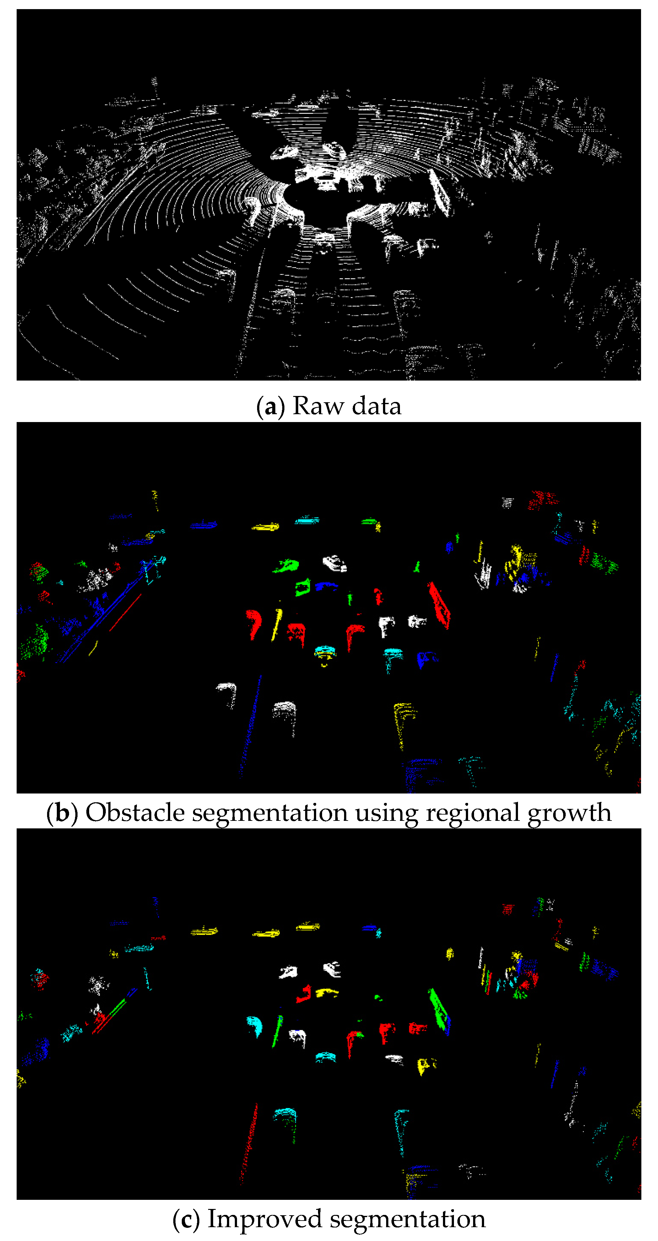
3.1. Object Segmentation
- Unstable objects, such as low curbs and branches of trees, are eliminated directly by the threshold of both grid height and object height. The gird height is calculated by maximum height and minimum height difference of points in one grid, and the object height is calculated by maximum height and minimum height difference of grids in one object.
- Objects such as the trees, street lamps, and road signs in the environment are stable, feature-obvious, and not easily shadowed. They are important features in the registration. The height of such objects is usually very different from that of the surrounding objects, so they can be separated from other objects according to the height difference between adjacent grids.
- height information is introduced to denoise the point cloud according to the object height
- more reasonable point cloud segmentation using height difference between grids
- compulsive segmentation of large objects
3.2. Registration
3.2.1. Overview
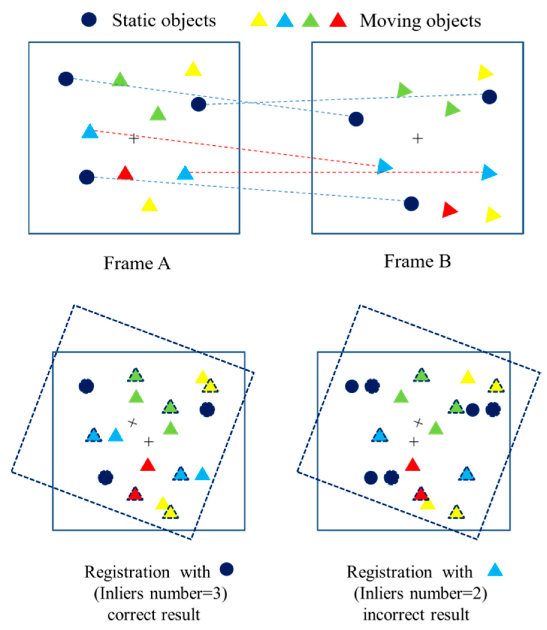
3.2.2. Data Association
3.2.3. Multi-Layer RANSAC
| Algorithm 1 Multi-layer RANSAC | |
| Step | Description of the implementation of the Multi-layer RANSAC algorithm |
| 1 | Start: |
| 2 | K: KNN search parameter |
| 3 | Ncp: Number of correspondences in set A and Bj |
| 4 | : Threshold of inliers ratio |
| 5 | Fori = 0 to L do |
| 6 | K = K(i) |
| 7 | For j = 0 to N do |
| 8 | M = M(j) |
| 9 | For k = 0 to M do |
| 10 | RANSAC(A, Bj) |
| 11 | End for |
| 12 | Calculating Tj with the largest number of inliers |
| 13 | T = T·Tj |
| 14 | Rj = max(nk)/Ncp |
| 15 | If then |
| 16 | Return T |
| 17 | Else |
| 18 | Bj+1 = Tj (Bj) |
| 19 | End if |
| 20 | End for |
| 21 | End for |
| 22 | RANSAC(A, Bj): |
| 23 | Random sample pi in A |
| 24 | Search correspondences of pi in Bj by KNN |
| 25 | Pick the points that satisfy conditions |
| 26 | Calculate matrix of each corresponding pairs |
| 27 | Transform Bj and count the number of inliers |
| 28 | End. |
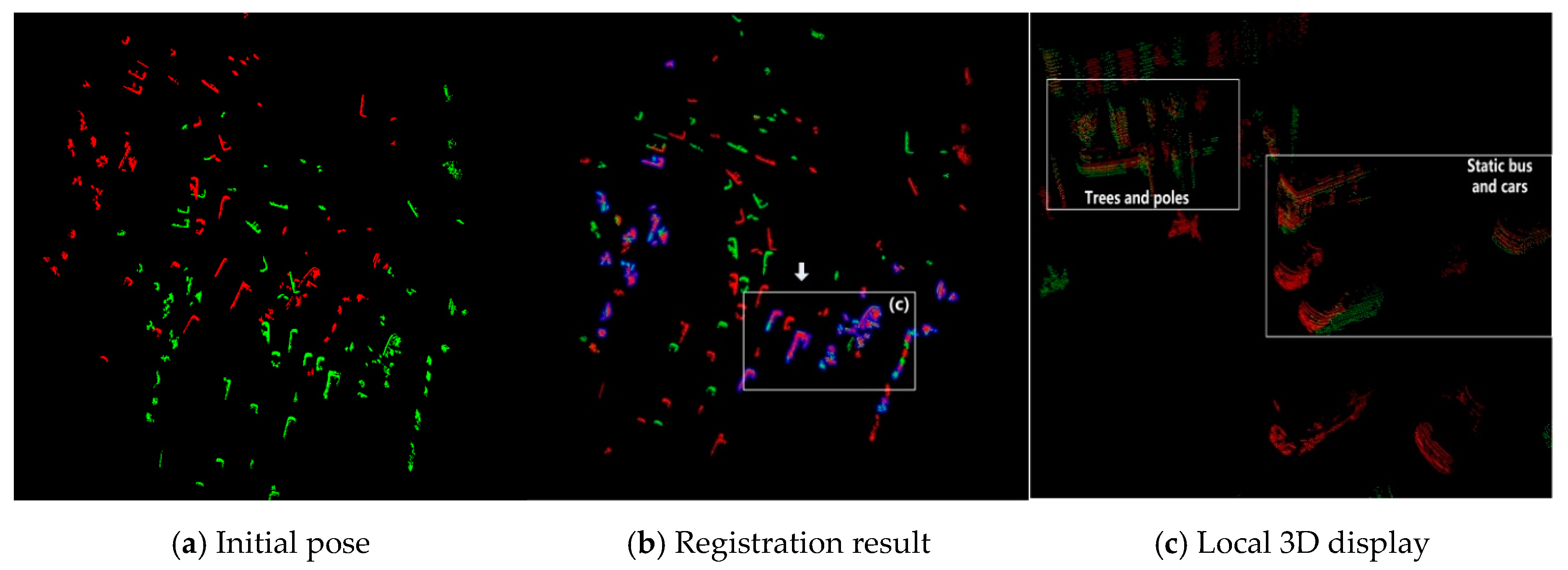
3.2.4. Accurate Registration
4. Experiments
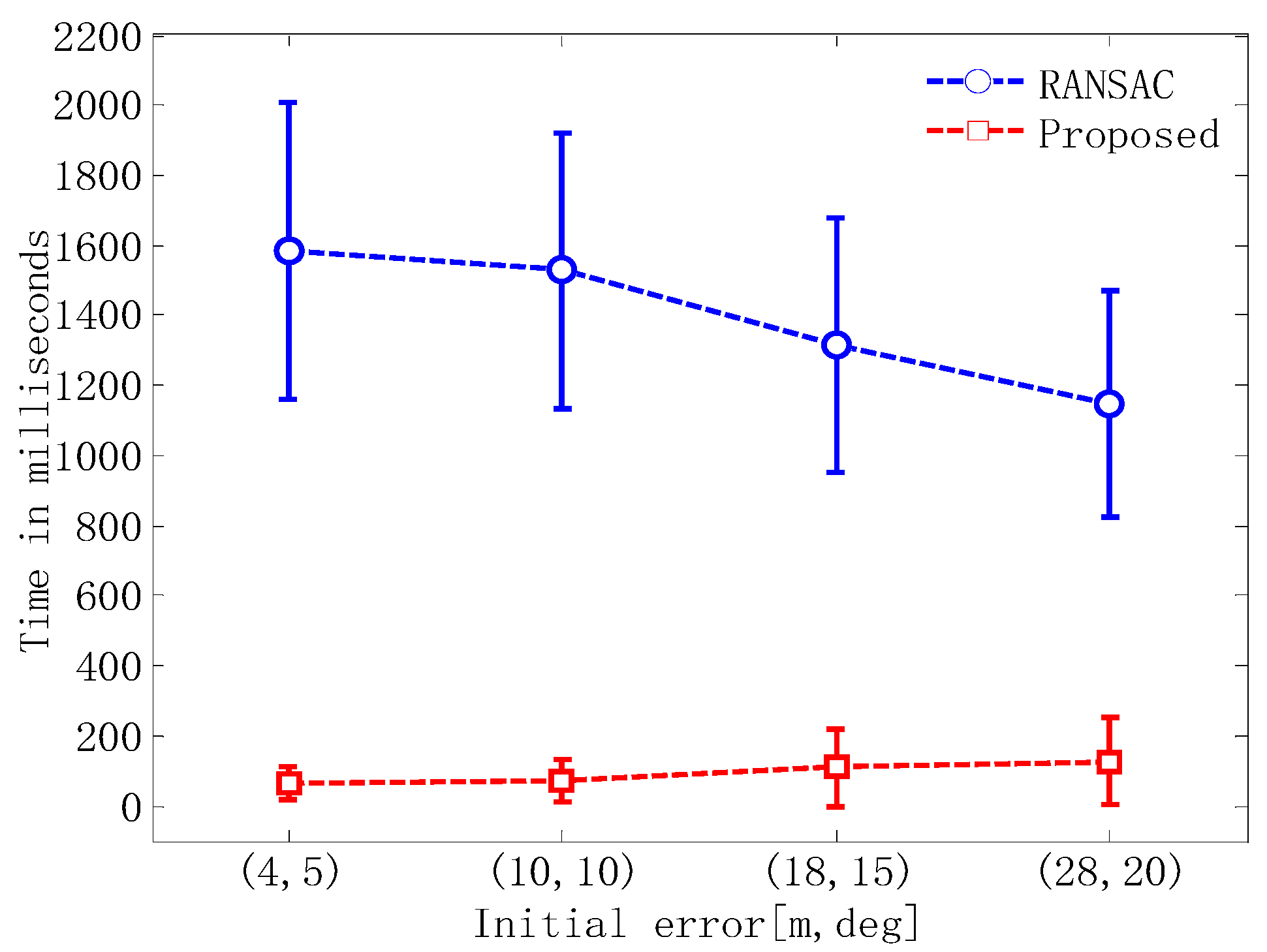
4.1. Registration
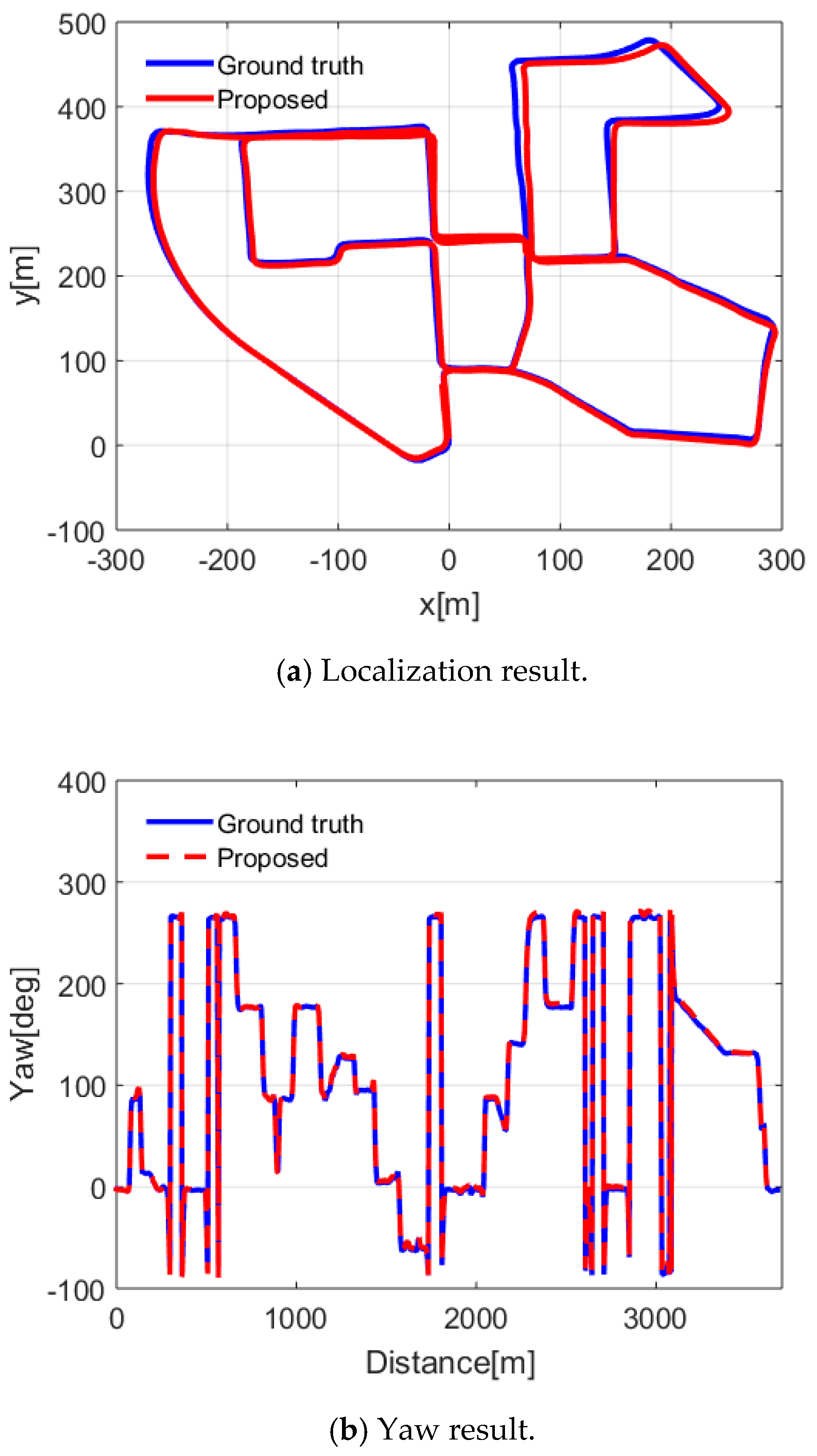
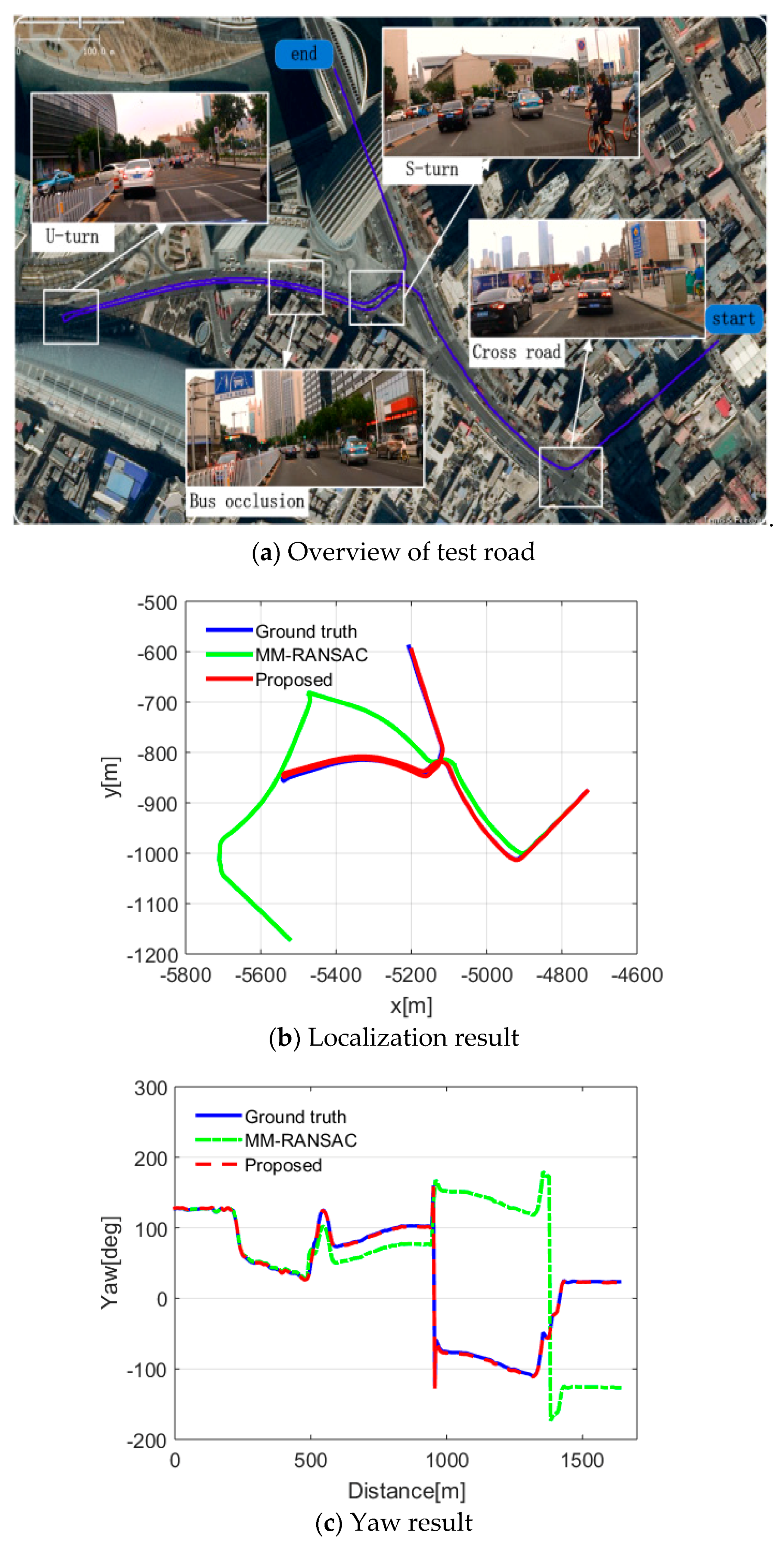
4.2. LiDAR Odometry
5. Conclusions
Supplementary Materials
Author Contributions
Funding
Acknowledgments
Conflicts of Interest
References
- Levinson, J.S. Automatic Laser Calibration, Mapping, and Localization for Autonomous Vehicles. Ph.D. Thesis, Stanford University, Stanford, CA, USA, 2011. [Google Scholar]
- Wolcott, R.; Eustice, R. Fast LIDAR Localization using Multiresolution Gaussian Mixture Maps. In Proceedings of the 2015 IEEE International Conference on Robotics and Automation (ICRA), Seattle, WA, USA, 26–30 May 2015; IEEE: New York, NY, USA, 2015; pp. 2814–2821. [Google Scholar]
- Zhang, J.; Singh, S. Low-drift and real-time lidar odometry and mapping. Auton. Robots 2017, 41, 401–416. [Google Scholar] [CrossRef]
- Cadena, C.; Carlone, L.; Carrillo, H.; Latif, Y.; Scaramuzza, D.; Neira, J.; Reid, I.; Leonard, J. Past, present, and future of simultaneous localization and mapping: Towards the robust-perception age. IEEE Trans. Robot. 2016, 32, 1309–1332. [Google Scholar] [CrossRef]
- Chum, O.; Matas, J.; Kittler, J. Locally Optimized RANSAC. In Proceedings of Joint Pattern Recognition Symposium; Springer: Berlin/Heidelberg, Germany, 2003; pp. 236–243. [Google Scholar]
- Sattler, T.; Leibe, B.; Kobbelt, L. SCRAMSAC: Improving RANSAC’s Efficiency with a Spatial Consistency Filter. In Proceedings of the 2009 IEEE International Conference on Computer vision, Kyoto, Japan, 29 September–2 October 2009; IEEE: New York, NY, USA, 2009; pp. 2090–2097. [Google Scholar]
- Pankaj, D.; Nidamanuri, R. A robust estimation technique for 3D point cloud registration. Image Anal. Stereol. 2016, 35, 15–28. [Google Scholar] [CrossRef]
- Moosmann, F.; Stiller, C. Joint Self-Localization and Tracking of Generic Objects in 3D Range Data. In Proceedings of the 2013 IEEE International Conference on Robotics and Automation, Karlsruhe, Germany, 6–10 May 2013; IEEE: New York, NY, USA, 2013; pp. 1146–1152. [Google Scholar]
- Yang, S.; Wang, C. Multiple-model RANSAC for Ego-Motion Estimation in Highly Dynamic Environments. In Proceedings of the 2009 IEEE International Conference on Robotics and Automation, Kobe, Japan, 18 August 2009; IEEE: New York, NY, USA, 2009; pp. 3531–3538. [Google Scholar]
- Wang, C.; Thorpe, C.; Thrun, S.; Hebert, M.; Durrant-Whyte, H. Simultaneous localization, mapping and moving object tracking. Int. J. Robot. Res. 2007, 26, 889–916. [Google Scholar] [CrossRef]
- Fischler, M.A.; Bolles, R.C. Random sample consensus: A paradigm for model fitting with applications to image analysis and automated cartography. Commun. ACM 1981, 24, 381–395. [Google Scholar] [CrossRef]
- Schlichting, A.; Brenner, C. Vehicle localization by lidar point correlation improved by change detection. Int. Arch. Photogramm. Remote Sens. Spat. Inf. Sci. 2016, 41, 703–710. [Google Scholar] [CrossRef]
- Im, J.; Im, S.; Jee, G. Vertical corner feature based precise vehicle localization using 3D LIDAR in urban area. Sensors 2016, 16, 1268. [Google Scholar] [CrossRef] [PubMed]
- Hata, A.; Wolf, D. Road Marking Detection using LIDAR Reflective Intensity Data and its Application to Vehicle Localization. In Proceedings of the 2014 IEEE International Conference on Intelligent Transportation Systems, Qingdao, China, 8–11 October 2014; IEEE: New York, NY, USA, 2014; pp. 584–589. [Google Scholar]
- Hata, A.; Osorio, F.; Wolf, D. Robust Curb Detection and Vehicle Localization in Urban Environments. In Proceedings of the 2014 IEEE Intelligent Vehicles Symposium, Dearborn, MI, USA, 8–11 June 2014; IEEE: New York, NY, USA, 2014; pp. 1257–1262. [Google Scholar]
- Aiger, D.; Mitra, N.; Cohen-Or, D. 4-points congruent sets for robust pairwise surface registration. ACM Trans. Gr. 2008, 27, 85. [Google Scholar] [CrossRef]
- Mellado, N.; Aiger, D.; Mitra, N. Super 4pcs fast global point cloud registration via smart indexing. Comput. Gr. Forum 2014, 33, 205–215. [Google Scholar] [CrossRef]
- Su, Z.; Xu, Y.; Peng, Y. Enhanced detection method for structured road edge based on point clouds density. Automot. Eng. 2017, 39, 833–838. [Google Scholar]
- Dimitrievski, M.; Van Hamme, D.; Veelaert, P.; Philips, W. Robust matching of occupancy maps for odometry in autonomous vehicles. In Proceedings of the 11th Joint Conference on Computer Vision, Imaging and Computer Graphics Theory and Applications (VISIGRAPP 2016), Rome, Italy, 27–29 February 2016; Volume 3, pp. 626–633. [Google Scholar]
- Anderson, S.; Barfoot, T.D. RANSAC for Motion-Distorted 3D Visual Sensors. In Proceedings of the 2013 IEEE/RSJ International Conference on Intelligent Robots and Systems (IROS), Tokyo, Japan, 3–7 November 2013; IEEE: New York, NY, USA, 2013; pp. 2093–2099. [Google Scholar]
- Geiger, A.; Lenz, P.; Stiller, C.; Urtasun, R. Vision meets robotics: The KITTI dataset. Int. J. Robot. Res. 2013, 32, 1231–1237. [Google Scholar] [CrossRef]


| Test A (Short-Term Registration) | Test B (Long-Term Registration) | |||
|---|---|---|---|---|
| Success | Fail | Success | Fail | |
| Error less than (0.2 m, 0.2 m, 0.5°) | 4126 | 40 | 3561 | 17 |
| Error more than (0.2 m, 0.2 m, 0.5°) | 29 | 2205 | 451 | 2371 |
| Scene | RMSE | ||
|---|---|---|---|
| Lateral (m) | Longitudinal (m) | Yaw(°) | |
| A1 turning right | 0.0148 | 0.0354 | 0.0954 |
| A2 turning left | 0.0298 | 0.0348 | 0.1113 |
| A3 bus occlusion | 0.0193 | 0.0753 | 0.2322 |
| A4 traffic jam | 0.0291 | 0.0249 | 0.0419 |
| B1 straight road | 0.076 | 0.1561 | 0.2751 |
| B2 cross road | 0.0342 | 0.044 | 0.0409 |
| B3 entrance ramp | 0.0546 | 0.0642 | 0.2328 |
| B4 elevated road | 0.0221 | 0.0373 | 0.047 |
© 2019 by the authors. Licensee MDPI, Basel, Switzerland. This article is an open access article distributed under the terms and conditions of the Creative Commons Attribution (CC BY) license (http://creativecommons.org/licenses/by/4.0/).
Share and Cite
Wang, R.; Xu, Y.; Sotelo, M.A.; Ma, Y.; Sarkodie-Gyan, T.; Li, Z.; Li, W. A Robust Registration Method for Autonomous Driving Pose Estimation in Urban Dynamic Environment Using LiDAR. Electronics 2019, 8, 43. https://doi.org/10.3390/electronics8010043
Wang R, Xu Y, Sotelo MA, Ma Y, Sarkodie-Gyan T, Li Z, Li W. A Robust Registration Method for Autonomous Driving Pose Estimation in Urban Dynamic Environment Using LiDAR. Electronics. 2019; 8(1):43. https://doi.org/10.3390/electronics8010043
Chicago/Turabian StyleWang, Rendong, Youchun Xu, Miguel Angel Sotelo, Yulin Ma, Thompson Sarkodie-Gyan, Zhixiong Li, and Weihua Li. 2019. "A Robust Registration Method for Autonomous Driving Pose Estimation in Urban Dynamic Environment Using LiDAR" Electronics 8, no. 1: 43. https://doi.org/10.3390/electronics8010043
APA StyleWang, R., Xu, Y., Sotelo, M. A., Ma, Y., Sarkodie-Gyan, T., Li, Z., & Li, W. (2019). A Robust Registration Method for Autonomous Driving Pose Estimation in Urban Dynamic Environment Using LiDAR. Electronics, 8(1), 43. https://doi.org/10.3390/electronics8010043