Short Term Residential Load Forecasting: An Improved Optimal Nonlinear Auto Regressive (NARX) Method with Exponential Weight Decay Function

Abstract

The advancement in electrical load forecasting techniques with new algorithms offers reliable solutions to operators for operational cost reduction, optimum use of available resources, effective power management, and a reliable planning process. The focus is to develop a comprehensive understanding regarding the forecast accuracy generated by employing a state of the art optimal autoregressive neural network (NARX) for multiple, nonlinear, dynamic, and exogenous time varying input vectors. Other classical computational methods such as a bagged regression tree (BRT), an autoregressive and moving average with external inputs (ARMAX), and a conventional feedforward artificial neural network are implemented for comparative error assessment. The training of the applied method is realized in a closed loop by feeding back the predicted results obtained from the open loop model, which made the implemented model more robust when compared with conventional forecasting approaches. The recurrent nature of the applied model reduces its dependency on the external data and a produced mean absolute percentage error (MAPE) below 1%. Subsequently, more precision in handling daily grid operations with an average improvement of 16%–20% in comparison with existing computational techniques is achieved. The network is further improved by proposing a lightning search algorithm (LSA) for optimized NARX network parameters and an exponential weight decay (EWD) technique to control the input error weights.

1. Introduction

Short Term Load Forecasting has ended up one of the major research fields in power system designing. With the recent changes in weather conditions determining power operation costs, the demand response and future load are more essential today than ever before. A power system operates by coordinating numerous stakeholders who can be influenced by an inaccurate forecasting estimate: Generation planning required a 24–48 h demand forecast in order to allocate the power resources economically [1]. The consumer can know energy prices and response based on the forecasted demand. The transmission sector ought to know the transmitted power necessities in order to allot assets, plan load shedding, draft commercialization strategies, and do risk management and contingency planning, which are all affected by the accuracy of load forecasting. Error in forecasted load can result in increase of operating cost [2]. Overestimation of demanded load will result in significant speculation for the development of abundance power sources while underestimation of demand will result in deficiencies and customer disappointment.

Generally, forecasting is divided into three main categories mainly determined by the forecasting period: long; medium, and short terms, respectively.

Short-term forecasting is based more on climate conditions such as dry bulb temperature, wet bulb temperature, humidity, and dew point temperature. Usually, the estimate load is from an hour to a week and is pivotal in generation scheduling or shutdowns, network flow rate optimization etc. Forecasting for medium-term and long-term depend more on financial variables and political choices. Medium-term lasts from a week to a year and is utilized for apportioning assets, arranging operations and establishing economic components such as tariffs, rate plans, and regulations. Long-term is generally for more than a year. A long time prediction is valuable for arranging the generation assets that need to be accessible at any point in time and extending them when required [3]. Experts for forecasting utilize numerous methods with each having a certain advantage and disadvantage [4]. Load forecasting techniques can be categorized in three sections, the statistical or parametric approach, a combination of statistical and computational methods, and intelligent computational techniques. The expert system, fuzzy logic, and the neural network are among the commonly-used computational intelligent techniques [5]. Ordinary load variations are not linear and, thus, non-linear networks have demonstrated high success in generating accurate short-term estimates. Neural Networks (NN) gave an exact perspective to the solve nonlinear problem and have the benefit of not necessarily having a thorough understanding of the inputs and output fundamental relationship. NN can be a crossover strategy that employs regression and dynamic time series. The NN observe past data information and finds patterns from that information. It employs that information to foresee the load demand using forecasted weather data. There are diverse structures for NN utilized to anticipate load, such as backpropagation, Boltzmann machines and Hopfield. Backpropagation is a commonly used NN technique for load forecasting. Contrary to statistical techniques, the mathematical model for NN is not required to be characterized “a priori.” The input layer can easily incorporate important parameters as a node and the network learns the relationship among parameters. Numerous creators [6,7,8,9,10] have analyzed the outcomes of distinctive artificial neural network (ANN) strategies. ANN has demonstrated an improvement in forecasting error and proved to be an effective forecaster when compared with corresponding statistical methods. This paper focuses on the range of expected accuracy obtained by comparing existing statistical, computational, and ANN techniques. The research meets at the junction of load forecasting, time-series forecasting, and ANN. The focus lies on short-term load forecasting utilizing ANN.

A unique and improved NARXNN based recurrent load forecaster is developed using the lighting search algorithm, which determines the optimal value for the number of hidden layer neurons, feedback delays, and input delays. This paper develops a recurrent neural network (RNN) with an LSA optimization algorithm to increase the robustness and intelligence of the forecasting method. The other heuristic optimization techniques such as particle swarm optimization, genetic algorithm, and simulated annealing are considered in pre-study due to the superiority of LSA in terms of speed, convergence, and error reduction. Only LSA is considered and explained in the proposed solution.

1.1. Literature Review

Bennett et al. [11] performed a comparison between ARIMAX and a multilayer feed forward network (MLFFN) to forecast a head peak demand and energy use. The hybrid model incorporated linear and quadratic multipliers for temperature and humidity parameters in the ARIMAX model. The MAPE for ARIMAX and ANN model calculated is in a range of 7% and 6%, respectively. Data is taken for 128 residential houses with introduction of dual exponential regression techniques to analyze the data trend. The hybrid mix of ANN-ARIMAX further improved the fit and accuracy. Hernandez et al. [12] took three layer MLFFN to forecast the regional load in Spain. Bayesian backpropagation is utilized for training. The hidden neurons are optimally determined by using a heuristic method. Averagely MAPE is 2.4%, which reached to 4% on specific days. Another work [13], forecasted city load by using two different MLFFN models. The output from a first conventional MLFFN model is fed to a modified two-stage second model to determine the day ahead load peaks and valleys. MAPE reduced from 2.4% to 1.6% in the modified model.

A support vector regression ANN model (SVR) is used by Fattaheian et al. [14]. Backpropagation is used to train a biased radial function. Initially, regression is executed by means of SVR then four different kernels, i.e., polynomial, linear, radial, and sigmoid are tested for better accuracy. The problem is solved optimally and is associated with a combinatorial model to obtain the lowest error. A fuzzy logic algorithm is used by Mahmoud et al. [15], which utilized post-processed output from a conventional forecaster with additional inputs to determine its output. This made the system more robust and covered all the missing data information. The model converged to a defined range, which optimized the error by functioning like a PI controller. The proposed technique is applied to MLFFN, SVR, and the FBTFS network improved MAPE to 4.2%, 4.9%, and 4.5%, respectively. Clustering regression is used in Reference [16] for Short Term Load Forecasting by multiple tests on time series data. The proposed regression and clustering stages proved more robust than conventional estimators. Authors in References [17,18] ensemble load patterns together by proposing a grouped framework of ANN, parameter estimation, and clustering. Currently, forecasting the load peak is also very critical since it effects significantly in the power system improvement and regional economic stability. Researchers have demonstrated keen interest to foresee such an event in Reference [19]. A data mining scheme is proposed for peak detection using a pattern recognition method instead of a time series approach. The algorithm demonstrated accuracy of 96.2% in day ahead peak detection. In Reference [20], variability of household behavior is analyzed using grade correspondence analysis with a post clustering approach. The electricity usage regularity is analyzed and the method is tested for 46 household data from Austin Texas, USA. In Reference [21], the neural network has been utilized to solve the nonlinear load-forecasting problem for economic generation planning. A leader following algorithm is utilized in 20 dimensions and shown high accuracy when compared with other forecasting algorithms in 2, 3, 5, 10, and 20 dimensions.

Ekonomou et al. [22] considered the de-noising wavelet algorithm to improve the accuracy for a hybrid model in order to neutralize input data before feeding it to a feedforward neural network. A comparison of two training algorithms, i.e., Levenberg–Marquardt and gradient decent with three different activation functions is done in Reference [23]. Different combinations of hidden layers and neurons are tested to analyze model performance on a yearlong real time data from Greece. A prediction accuracy test is performed in Reference [24] using the NARX ANN method on ERCOT data. Different training algorithms are used with varying lengths of training data set, effects of size, and the number of hidden layers are analyzed on network performance. Recently, heuristic and Meta heuristic optimization methods are extensively deployed to handle foresting problems. These methods are stochastic in nature and perform according to a natural phenomenon such as evolution, natural selection, and self-grouping. LSA is maintaining dominance among these techniques in terms of speed, convergence, and error reduction. The LSA search for the best solution using fast searching projectiles mimicking natural lighting process. A study [25] with 24 benchmarks and multiple characteristic functions is performed to test the robustness and efficiency of LSA. The result demonstrated LSA reliability. Krogh et al. [26] utilized the linear weight decay method in the predicted model and successfully tested its performance. The authors in References [27,28] presented a general improvement in the model by masking the error weights.

1.2. Contributions

The paper presented a strategy of attaining a more precise short-term residential load forecast utilizing a recursive ANN approach with varying climate factors as exogenous input vectors. A fully connected neural network with 10 hidden layers and a logistic sigmoid as an activator in hidden nodes and linear activator in output nodes forecasts a 24-h output as the yield. The input vector incorporates month, day, the specific day of the week, working day or holiday, climate information, and historical load data as an exogenous input. Some available algorithms to train NN are: Bayesian regularization, Levenberg-Marquardt, gauss-newton, and gradient decent. In the proposed method, the weight of hidden layers are updated by using the Levenberg-Marquardt algorithm. The node weights are calculated by training the network in an open loop, utilizing existing load data, and then the forecasted load is utilized as an input in a close-loop to the regenerate forecast. Due to network recurrent behavior, it will reutilize its calculated output and will not require retraining in order to proceed to provide the forecast. The results show a notable development when compared with statistical methods i.e., ARMAX and state space, Decision Tree i.e., BRT and conventional feedforward ANN FitNet method without exogenous inputs. The proposed method does encounter stability issue generated during the closed loop, used optimal value for feedback, and input the time lag. The proposed method is further furnished by applying a unique and improved NARXNN based recurrent load forecaster using a lighting search algorithm (LSA), which determines the optimal value for the number of hidden layer neurons, feedback delays, and input delays. Moreover, an error decay method is employed and gives more weight to the error from recent data and exponentially decreases the error weight from lagged data. The final outcome of the proposed method is compared with the results from two training algorithms i.e., Bayesian regularization and Levenberg-Marquardt and two activation function i.e., Hyperbolic Tangent and Logistic Sigmoid with and without an exponential decay function to demonstrate the chosen parameters’ efficiency.

1.3. Organization

The remainder of the manuscript is prepared as follows: Section 2 sheds light on the nature of the data with Pearson correlation analysis of different input parameters. A brief introduction about the reference forecasting methods is presented in Section 2 with introduction about foresting methods in Section 3. The proposed framework is thoroughly analyzed in Section 4. The performance evaluation of the proposed model with comparative analysis is presented in Section 5. The discussion on results is presented in Section 6 and the conclusion is drawn in the last section.

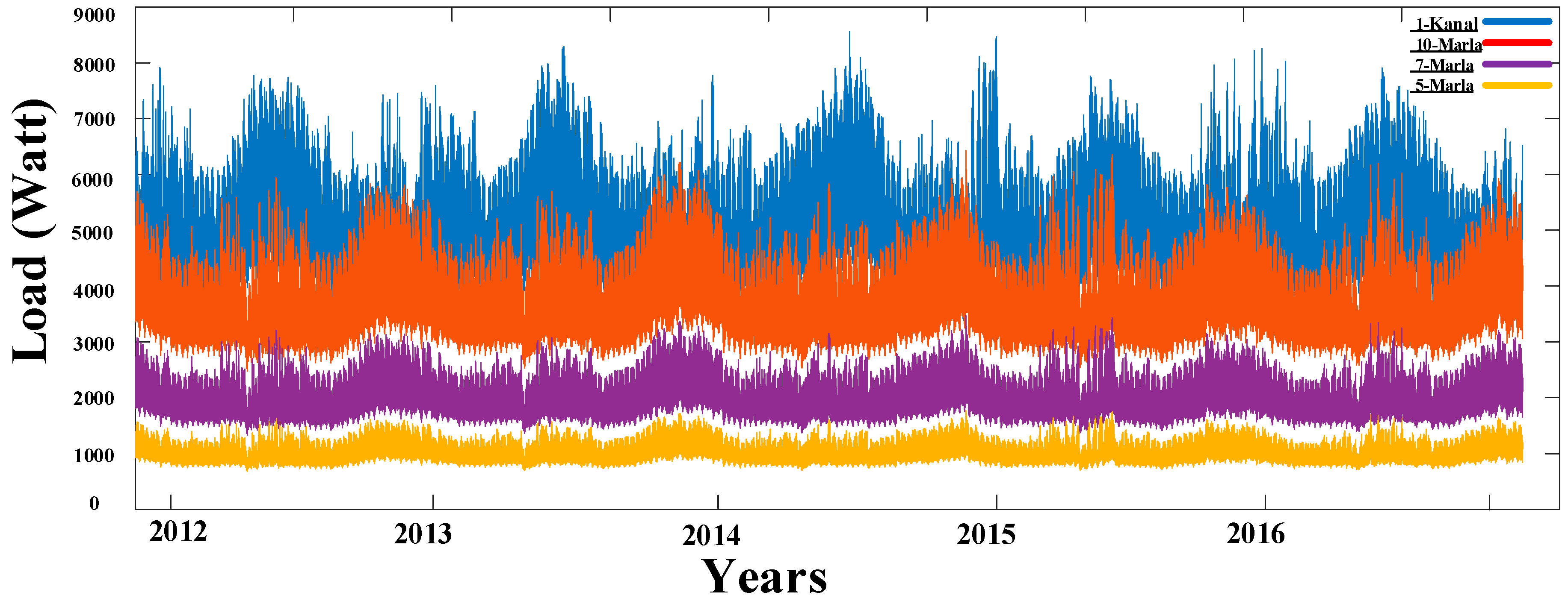
2. Load Consumption IESCO

Islamabad is the capital city of Pakistan and has developed infrastructure with the number of residential load zones. The city has an extensive socio-economic growth in past decades and, with the same pace of development, the EVs will become a considerable common household load with a prominent grid impact. The electrification responsibility of the region is under Islamabad electric supply company IESCO, which is a state owned distribution firm. The power demand for Pakistan is experiencing a steep increase and it becomes very important to estimate the forecasted load accurately in order to satisfy the customer needs as well as properly plan and build the power system infrastructure. In this paper, the IESCO data for active power consumption of different residential units is analyzed. The houses are categorically divided into four types depending on their power consumption and occupied land area. The details of minimum and maximum demand in the winter and summer and specific names associated with each type are as follows:

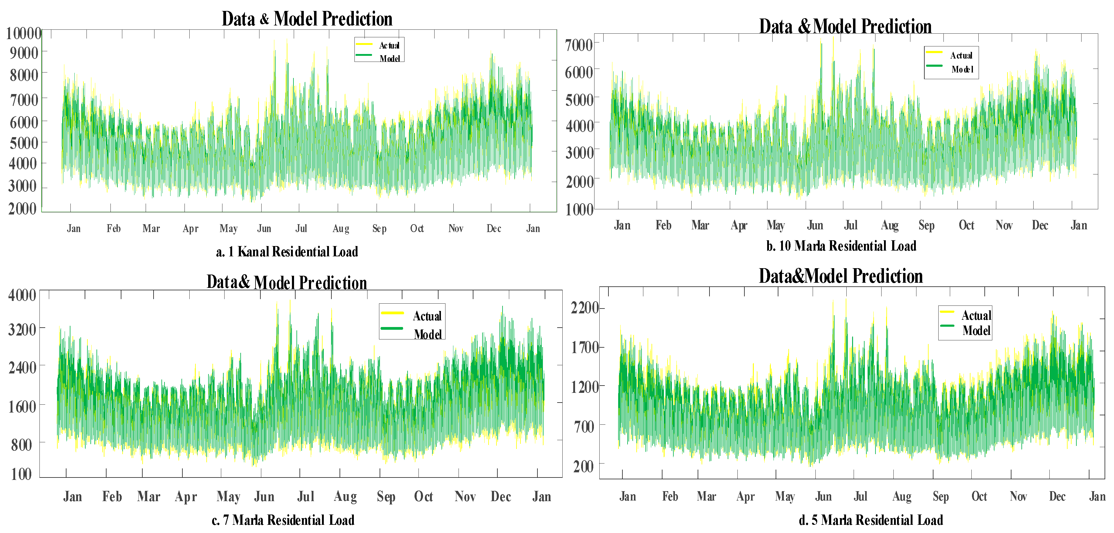
• 1 Kanal = 10,042 Square Meter approx., Load Demand; winter (3.5 kW–8.5 kW); Summer (2.5 kW–8 kW)
• 10 Marla = 5021 Square Meter approx., Load Demand; winter (2.5 kW–6.5 kW); Summer (2 kW–6 kW)
• 7 Marla = 3514 Square Meter approx., Load Demand; winter (1 kW–3.5 kW); Summer (1 kW–3kW)
• 5 Marla = 2510 Square Meter approx., Load Demand; winter (0.5 kW–2 kW); Summer (0.5 kW–1.7 kW)

The hourly real-time data was collected from a substation in Islamabad for five years from 2012 to 2016 [29]. The substation caters only residential load. From data, it is analyzed that the time series load variations for residential consumers have strong seasonal and weather dependency. The yearly residential load profile, as shown in Figure 1, follows a specific seasonal pattern considering the 24-h profile. The summer morning peak appears from 07 to 10 h and the evening peak occurs from 15 to 20 h. In the winter, the morning peak is from 07 to 09 h and the evening peak period is from 17–21 h. The load profile for weekends follows a different trend unlike the working days. The monthly pattern analyzed for the summer and winter showed that the consumer peak demand is during the month of July in the summer and December in the winter, respectively, which shows strong seasonal influence on load variation.

Figure 2 shows the triangle plots for seasonal variations [30] (Dew Point & Dry Bulb Temperature) vs. Load. It can be seen that, during the winter, at a low temperature, there is a considerable rise in demand due to heating load and similarly the trend repeats for the summer due to the air conditioning load. The comfort zone is during the autumn and spring at around 20 to 24 °C when there is no heating and cooling load.

Variables like humidity, working hours, and temperature were considered to find the variations in load trends. The Pearson correlation shown in Figure 3 of all chosen predictors is analyzed and only significant variables with a 90% confidence interval is used since it can been seen that the wet bulb has the same effect on the load as dew point temperature. Therefore, it is not considered as an input vector in the model.

3. Load Forecasting Methods

Short Term Load Forecasting (STLF) can be methodically categorized into three sections based on past studies.

Statistical Methods, Statistical-Computational Methods, and Intelligent Computational Methods.

LF is largely a nonlinear regression issue and the connections between diverse factors are examined with the assistance of historical data samples [31]. With the following concept, distinctive sorts of STLF models with a shifting success ratio are created. Numerous components particularly time periods, climatic changes, and the air condition are considered as a part of the model. The technique and the precision of the LF model change due to a given situation.

3.1. Statistical Methods

Statistical strategies incorporate all forms of parametric and autoregressive models. Nonlinear relationships are attempted to distinctly model by utilizing regression techniques, which act as linear devices. When nonlinear regression is utilized, the relationship between the required output and the illustrative inputs is exceptionally complex and it is difficult to approve observationally.

The common statistical methods utilized for the short-term load forecasting are shown below [32,33].

• ARMA-Auto Regress Moving Average
• ARIMA-Auto Regress Integrated Moving Average
• State Space
• Linear Regression

ARIMA/State Space

To begin with, the ARIMA prerequisites must be met and a prior information transformation needs to be performed. ARIMA models are the foremost non-linear general class models for forecasting time series data. The most necessity for the data while applying the ARIMA model is that the data must be stationary, i.e., the data characteristics must not be subordinate on which time outline is chosen. This implies that there must be no patterns within the data or any predictable reaction on the model residuals. Diverse strategies for making the data stationary are utilized including the favorable ones of which are deflating or logging differences. The objective to achieve with this change is to attain a data set in which its autocorrelations stay consistent over time. We must begin with recognizing the control range of the data series for the purpose to decide the natural frequencies that exist within the fundamental data. We apply the ARIMA model by performing the following steps.

• Apply quick Fourier transformation, remove trends, and ensure the model is stationary.
• Autocorrelation and partial autocorrelation graphs are analyzed to check if the moving average and autoregressive models are suitable. To confirm ARMA configuration, check for the extended data autocorrelation graph.
• Different ARMA model sets are tested for the lowest Akaike’s Information (AIC) and Schwartz Bayesian Information (BIC) Criterion.

The ARIMA model is developed by using the model optimizer in SPSS, the optimal parameters found are AR = 2, I = 1, and MA = 8, which is an autoregressive model of second order, the differences of one degree, and a moving average of the eighth degree. The fitting error is reduced from the output using proposed ARIMA configuration in Expert Modeler platform of SPSS. The resulting ARIMA model is further transformed to generate a state space model for a comparison purpose. This fitting produce does not necessarily confirm a good forecasting output since a lot of periodic data information is left in the residuals. An improvement is done by implementing the proposed neural network model. The result of this is presented in the simulation and result section.

3.2. Computational-Statistical Methods

In data mining, generally, the decision tree method is taken as a combination of statistical and computational techniques. It uses a tree predictive model and branches to represent the observation about an item and leaves to represent the target values. This approach is utilized in data mining, statistics, and machine learning. Decision trees are classified in two main types, which includes Regression tree and Classification tree, respectively. Some ensemble methods used to construct a multiple decision tree are as follows: Boosted trees; Bootstrap aggregated, and Rotation forest. In this paper, the bootstrap aggregated decision tree approach is utilized to test the performance of the proposed model.

Bootstrap Regression Tree

Bootstrap bagging or aggregation may be the most effective outfit strategy given by Leo Breiman, which exact individual model estimation by incorporating different machine learning tools [34]. Since a singletree is liable to over fit, bagging is utilized to diminish the fluctuation among calculations like regression trees. Nevertheless, the outcomes of numerous selected trees are combined by bagging to overcome the overfitting issue. The in-bag test samples, which represent each independent tree, are generated individually as a replica from the input data set. Almost one-third of out-of-bag test samples, which are an excluded dataset, are utilized for estimating the error in the forecast model. The input dataset is separated in two sets: training set 2012 to 2015 and test set 2015 to 2016. The training set is utilized for the model parameters estimation while the test set is utilized to check the forecasting model credibility. The forecast model with set of regression trees is built utilizing MATLAB Bagger Tree function with each individual tree performing regression with a diverse set of rules. Initially, 20 such trees with 40 least leaf estimates are utilized. The regression tree size is determined by the leaf size and the smaller trees have larger leaf size. The size of the tree measure provides the power to control performance execution and overfitting.

3.3. Computational Intelligent Methods

Computational intelligence (CI) strategies incorporate, expert system, fuzzy logic technique, and artificial neural systems (ANN). Typically, for the nonlinear load, these techniques are more compelling in producing a short-term forecast. Particularly, ANNs gave operators a freedom of not having basic numerical understanding of the issue and have the advantage of generating yield with less complexity. Recently, ANNs are compelling a forecasting technique among researchers. The results of different studies proved ANN held a statistical counterpart [35,36]. A brief description of ANN architecture is given in the section below.

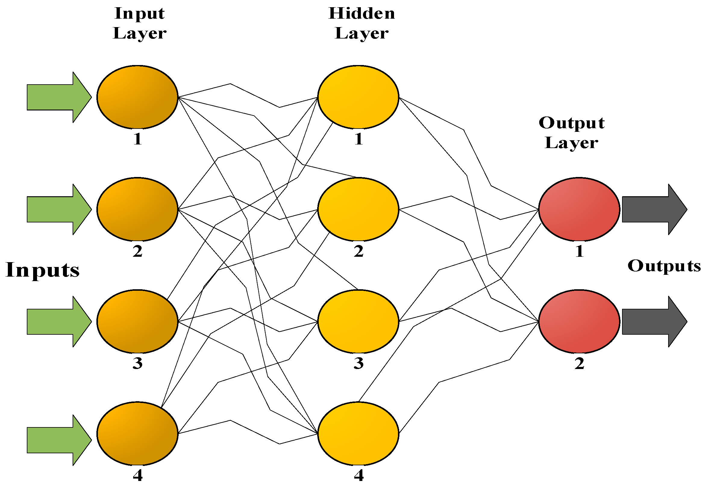
Artificial Neural Network (ANN) Description

An Artificial Neural Network is a nonlinear intelligent computational method of cross-connected neurons propelled by centrally controlled nervous system as in human creatures. The neuron is defined as a fundamental cell in ANN. Different neurons operate side by side to handle the mathematical information similar to a human brain. A fundamental network architecture demonstration is given in Figure 4 that is comprised of three crucial capacities: scalar weights, the summing intersections, and a transfer function, which produce scalar yield.

The numerical representation of a fundamental neural network is given below [37].

$$Y_l={{\displaystyle \sum }}_{l=1}^m{W}_l{P}_l$$

(1)

where $P_l$ represents the kth input, $W_l$ is the weight designated to lth input, and $Y_l$ is lth yield of ANN and l = 1, 2, 3, …, m.

The parallel neurons get mathematical information and handle it in two steps. Directly duplicate the value with weights $W_l$ and forward the weighted values to summing the intersection that appeared in Figure 5. The intersections are represented by circles. A comprehensive study on ANNs is displayed in Reference [38].

Artificial intelligence-based models are considered more solid, adaptable, and precise in comparison with regular regression-based strategies but need a huge set of information for data training and validation. However, regression techniques are commonly utilized when the accessibility of notable information may be a huge issue. In recent years, there is an increase in adaptation of AI-based estimating models among the analysts. ANNs is favored for the most part because of the inborn capacity to bargain with the nonlinearities among parameters such as the cyclic load behavior and weather changings, which are complicated to grasp in ordinary models [39]. NN is supplanting the conventional techniques utilized for day a head load and cost predictive analysis due to their straightforwardness and high accuracy. Most ANN strategies come about with a mean absolute percentage error (MAPE) of around 2% to 4% compared to statistical strategies, which produce an error within the range of 5% to 6%. The objective is to get a reliable estimate for the forecast error, which is lower than preferred statistical techniques. An SPSS and a Matlab information system was built up in order to generate forecasting results through a nonlinear statistical regression model, which can be utilized as a benchmark for examining the execution of the proposed ANN. The important features utilized in the proposed model to build a competent ANN model are explained in the proposed network section.

4. NARX Neural Network

The applied network is designed to take exogenous inputs i.e., weather and time variables and endogenous inputs i.e., electrical load, and give a 24-h load as an output. The general architecture of the NARX network is given below.

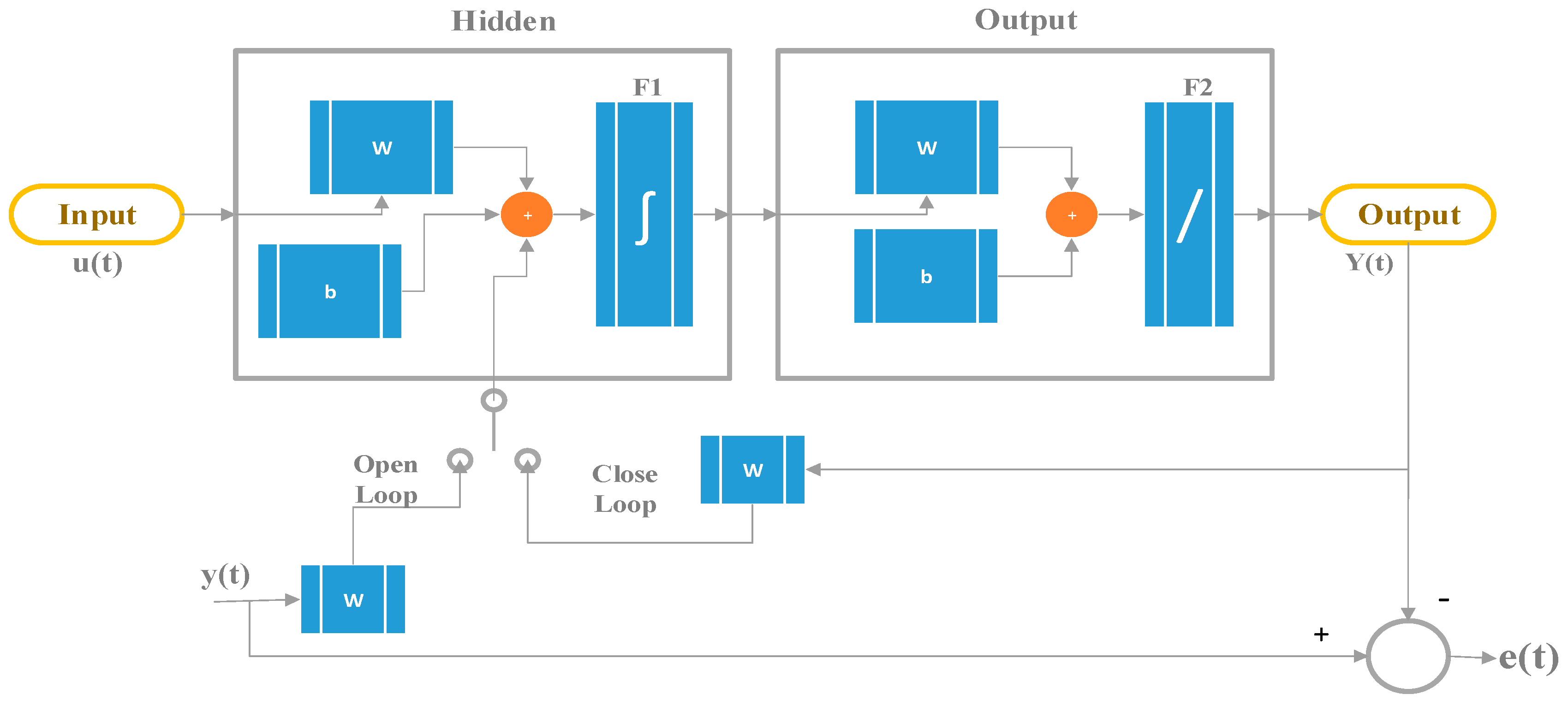
4.1. NARX Architecture

In general forecasting, the independent variable u has a cause-effect relationship with forecasted variable y, which can be represented by Equation (2). For time series, forecasting the previous outputs $y_t$ and previous time interval $y_{t-p}$ determine the output for the next interval and can be expressed by Equation (3). The time series model forecasting accuracy is improved by taking into account the predictors and time lagged variables as inputs to produce the output, which is defined by Equation (4).

$$y=f\left(u_1,u_2, \dots , u_n\right)$$

(2)

$$y_{t+1}=f\left(y_t,y_{t-1}, \dots , y_{t-p}\right)$$

(3)

$${\overrightarrow{y}}_{t+1}=f\left({\overrightarrow{u}}_1,{\overrightarrow{u}}_2,\dots , {\overrightarrow{u}}_p,{\overrightarrow{y}}_t,{\overrightarrow{y}}_{t+1}, \dots , {\overrightarrow{y}}_{t-q}\right)$$

(4)

In Equation (3), accuracy is improved by considering $u_p$ variables, which represents an external predictor vector along with ${\overrightarrow{y}}_{t-q}$. This represents a lagged output vector. ${\overrightarrow{y}}_t$ is a 24 × 1 output vector containing the day-a-head load forecast. In addition, it is important to keep in mind that each of the inputs is in itself a vector of different variables. In the present work, the exogenous predictors ${\overrightarrow{u}}_1,{\overrightarrow{u}}_2,\dots ,{\overrightarrow{u}}_p$ are the time and weather variables shown in Figure 1. The time-lagged vector variables ${\overrightarrow{y}}_t,{\overrightarrow{y}}_{t+1},\dots ,{\overrightarrow{y}}_{t-q}$ are the past values of the load. These variables are fed to the model in three vector streams as inputs: five-year hourly load values, last week’s hourly load values, and the last 24-h hourly load values. The justification of this overlap is to increase the weight of more recent values of the output variables over the oldest values. The Input-output relationship of ANN using NARX can be formulated as follows [40].

$$y\left(t\right)=F\left[u\left(t\right),u\left(t-\Delta t\right),\dots , u\left(t-n\Delta t\right),y\left(t\right),y\left(t-\Delta t\right), \dots ,y\left(t-m\Delta t\right)\right]$$

(5)

In this case, n and m represent the delay time step in input and fed back output, respectively, where F represents a nonlinear function. The actual values of load $y\left(t\right)$ are used to train the network and, in order to produce the forecasted 24-h load, the predicted $y\left(t\right)$ load values are fed back in a closed loop in a step of one hour. A backpropagation Levenberg–Marquardt training algorithm is used to train the network in open loop utilizing the previous 365 days of data consecutively. The last 24-h data is fed to the network as input in the closed loop mode while the fed back calculated the load produced output with hour increments.

While operating in a closed-loop, the well-known, time varying exogenous variables such as (working days, holidays, specific day in week, month, day, and hour) are utilized as regular inputs. However, the forecasted values of weather parameters (dry bulb and dew point temperatures) are taken for the chosen 24-h span where the load is being forecasted.

For a proposed framework, a feed forward perceptron neural network is constructed to study the behavior of output $y_t$ at time t, utilizing inputs $u_t$. The regression model for the output layer y is represented in a nonlinear functional form below.

$$y_t=\mathsf{\phi }\left[{\beta }_0+{{\displaystyle \sum }}_{i=1}^q{\beta }_i{h}_{it}\right]$$

(6)

In this scenario, the hidden layer $h_{it}$ is given as:

$$h_{it}=\mathsf{\Omega }\left[{\gamma }_{i0}+{{\displaystyle \sum }}_{j=1}^n{\gamma }_{ij}{x}_{jt}\right]$$

(7)

$\mathsf{\phi }$ is the output activation function, is linear, and is given as:

$$\mathsf{\phi }\left(\mathrm{x}\right)=\mathrm{x}$$

(8)

$\mathsf{\Omega }$ is the logistic sigmoid activation function for hidden neurons, which is of form:

$$\mathsf{\Omega }\left(\mathrm{t}\right)=\frac{1}{1+ e^{-t}}$$

(9)

The logistic function is utilized to limit or flatten the neuron weights. The bias value of output is represented by ${\beta }_0$. The output layer weights are represented by ${\beta }_i$ and input bias and weights of input layer are represented here by ${\gamma }_{i0}\mathrm{and}{\gamma }_{ij}$ respectively, where sub index of q neurons and n inputs are represented by i and j, respectively. From Equations (6) and (7), we have:

$$y_t=\mathsf{\phi }\{{\beta }_0+{{\displaystyle \sum }}_{i=1}^q{\beta }_i\mathsf{\Omega }\left[{\gamma }_{i0}+{{\displaystyle \sum }}_{j=1}^n{\gamma }_{ij}{x}_{jt}\right]\}$$

(10)

Then, for recurrent network description, an autoregressive, dynamic term is added on the output. The hidden layers are represented by the equation below.

$$h_{it}=\mathsf{\Omega }\left[{\gamma }_{i0}+{{\displaystyle \sum }}_{j=1}^n{\gamma }_{ij}{x}_{jt}+ {{\displaystyle \sum }}_{r=1}^q{\delta }_{ir}{h}_{r,t-1}\right]$$

(11)

Here, the delayed term weight is represented by ${\delta }_{ir}$ and the feedback term by $h_{r,t-1}$. Replacing Equation (11) into Equation (6), we obtain:

$$y_t=\mathsf{\phi }\{{\beta }_0+{{\displaystyle \sum }}_{i=1}^q{\beta }_i\mathsf{\Omega }\left[{\gamma }_{i0}+{{\displaystyle \sum }}_{j=1}^n{\gamma }_{ij}{x}_{jt}+ {{\displaystyle \sum }}_{r=1}^q{\delta }_{ir}{h}_{r,t-1}\right]\}$$

(12)

Equation (12) shows multiple inputs and past values of the output, which generally represents the dynamics of the network. However, the equation represents the model as having only one hidden neural layer, which can be extended to N layers by introducing the k index. Where $k=1, \dots , \tau$, and $\tau$ outputs have a multi-dimensional nature.

$$y_t^k=\mathsf{\phi }\{{\beta }_0^k+{{\displaystyle \sum }}_{l=1}^N{{\displaystyle \sum }}_{i=1}^q{\beta }_i^l\mathsf{\Omega }\left[{\gamma }_{i0}^l+{{\displaystyle \sum }}_{j=1}^n{\gamma }_{ij}^l{x}_{jt}+ {{\displaystyle \sum }}_{r=1}^q{\delta }_{ir}{h}_{r,t-1}\right]\}$$

(13)

Equation (13) represents the proposed NARX network. The network description for the open loop and the closed-loop only varies by the method through which the delayed output is drawn. In open-loop, the values of y is obtained from known historical output values and, taken as a regular network input but in a closed-loop case, the value of y is obtained from predicted output values. This description is given in Reference [11].

4.1.1. Non Recurrent or Recurrent Network

For feed forward topology, the proposed framework is trained initially in the open loop with a training data set containing historical hourly load and weather data. The network is made recurrent after feeding the output as an input into ANN, which is calculated after determining the node weights in the open loop. Figure 6 shows the proposed Nonlinear autoregressive network. Two position switches for open and close loop are shown. The switch is connected in the open loop phase during training and in the closed loop phase during forecasting where the future value is predicted by utilizing the calculated load values. The network weight is determined in the open loop during the training process since the actual load output y(t) is a known reason. During the forecasting phase in the closed loop, the actual load output is unknown. Therefore, the predicted load value with delay is fed back to the network to produce a forecasted value.

4.1.2. Optimal Parameters

The network optimal structure is determined by iterating the number of neurons and the best network with optimal fit is saved for forecasting purposes. However, for determining the optimal value for input and feedback lag, certain procedures are needed due to the model recursive nature. They are complicated to determine analytically.

The procedure can be categorized in three types. Direct method: Retrain the network until a minimum error is obtained (difficult to generalize error threshold, as network abilities are unknown and its time consuming to retrain). Select Stopping Criteria: by dividing the data into training, testing and validation set, a more consistent stopping criteria can be acquired. The training is stopped based on minimum error on the validation set. The error weight on the training set is continuously decaying but the error on validation set stops after decreasing to a minimum value until it increases again. When the error is at a minimum, on the validation set, the network and generalized characteristics are optimal and it determines a good fit. Using this approach, the need to retain the network for a fixed error threshold can be omitted since the optimal value for input and feedback lags are determined without utterly retraining the network. The general architecture for stopping criteria is shown in Figure 7. Meta Heuristic Optimization: Multiple heuristic optimization techniques such as particle swarm optimization, genetic algorithm, and simulated annealing are considered in the pre-study. However, due to superiority of LSA in terms of speed, convergence, and error reduction, only LSA is considered and explained in the proposed solution.

Lighting Search Algorithm

Lighting Search Algorithm (LSA) is a metaheuristic optimization technique invented in 2005 [25]. The optimal solution is determined by propagating the step leader particles known as projectiles.

▪

Projectiles Properties

The projectile velocity $v_p$ and kinetic Energy $E_P$ are given by the equation below.

$$E_P=\left(\left(\frac{1}{\sqrt{1-{\left(\frac{v_p}{c}\right)}^2}}\right)-1\right)m{c}^2$$

(14)

$$v_p={\left[1-{\left(\frac{1}{\sqrt{1-{\left(\frac{v_p}{c}\right)}^2}}-\frac{s{F}^i}{m{c}^2}\right)}^{-2}\right]}^{-\frac{1}{2}}$$

(15)

In this scenario, v₀ is initial velocity, v_p is current velocity, s represents the traveling path length of the projectile, m represents the particle mass, Fⁱ is the constant rate of ionization, and c is the speed of light.

In LSA, projectiles are divided into three categories, i.e., transition, space, and lead projectiles. Movement of the step leader and projectiles modeling are explained below.

▪

Transition State Projectile

Initially, a leader tip is created randomly whose probability density function (PDF) could be mathematically represented as:

$$f\left(x^T\right)=\{\begin{array}{c}\frac{1}{b-a} for a\le x^T\le b\\ 0 for x\langle a or x^T\rangle b\end{array}$$

(16)

$s{l}_i$ gives the step leader value with a and b as a solution space upper and lower bounds, solution space is represented as $SL=\left(s{l}_1;s{l}_2;s{l}_3;\dots ;s{l}_N\right)$, $E_{sli}$ gives tip energy of step leader whose initial value is given by the random value $x^T$ with a population of N with solution dimensions $p^T=\left(p_1^T;p_2^T;\dots ;p_N^T\right)$.

▪

Space State Projectile

When the N movement in step leader tips is observed, a random number model is generated with partial properties having exponential distribution and shaping parameter $\mu$. The position at step+1 of the space projectile is given as $p^S=\left(p_1^S;p_2^S;\dots ;p_N^S\right)$. The Exponential distribution PDF in this case is given as:

$$f\left(x^s\right)=\{\begin{array}{c}\frac{1}{\mu }{e}^{-\frac{x^s}{\mu }} for x^s\ge 0\\ 0 for x^s\le 0 \end{array}$$

(17)

The updated position at step+1 stating the distance between space and lead projectile with exprand as exponential random function is given as:

$$p_{i\left(new\right)}^s=p_i^s\pm exprand\left({\mu }_i\right)$$

(18)

Step leader expand to $s{l}_{i\left(new\right)}$ when appropriate results are achieved at step+1, with corresponding value for $p_{i\left(new\right)}^s$, if expansion of $p_{i\left(new\right)}^s$ surpass $s{l}_{i\left(new\right)}$ then the new leader changed into the lead projectile.

▪

Lead State Projectile

With $\sigma ;\mu$ as a scaling parameter and shaping parameter respectively a random number model is generated for lead projectile, with a normal distribution, given as:

$$f\left(x^L\right)=\frac{1}{\sigma \sqrt{2\pi }}{e}^{-\frac{{(x^L-\mu )}^2}{2{\sigma }^2}}$$

(19)

At step+1 the lead projectile updated position with norm and representing normal random function is given as:

$$p_{i\left(new\right)}^L=p_i^L\pm normrand\left({\mu }_L,{\sigma }_L\right)$$

(20)

▪

Forking Method

Forking in LSA occurred in two ways:

• With production of symmetrical channels due to collusion in nucleus, given as:

  $$\overline{p_i}=a+b-p_i$$

  (21)
  The one-dimensional original and opposite projectiles are represented by $p_i$ and $\overline{p_i}$, respectively, with a and b as boundaries, a satisfied fitness value is chosen by the forking leader in order to increase the method efficacy.
• After the number of propagation, the unsuccessful step leaders re-forward the energy. In such a case, a successful leader tip is expected to produce a channel to generate forking.

▪

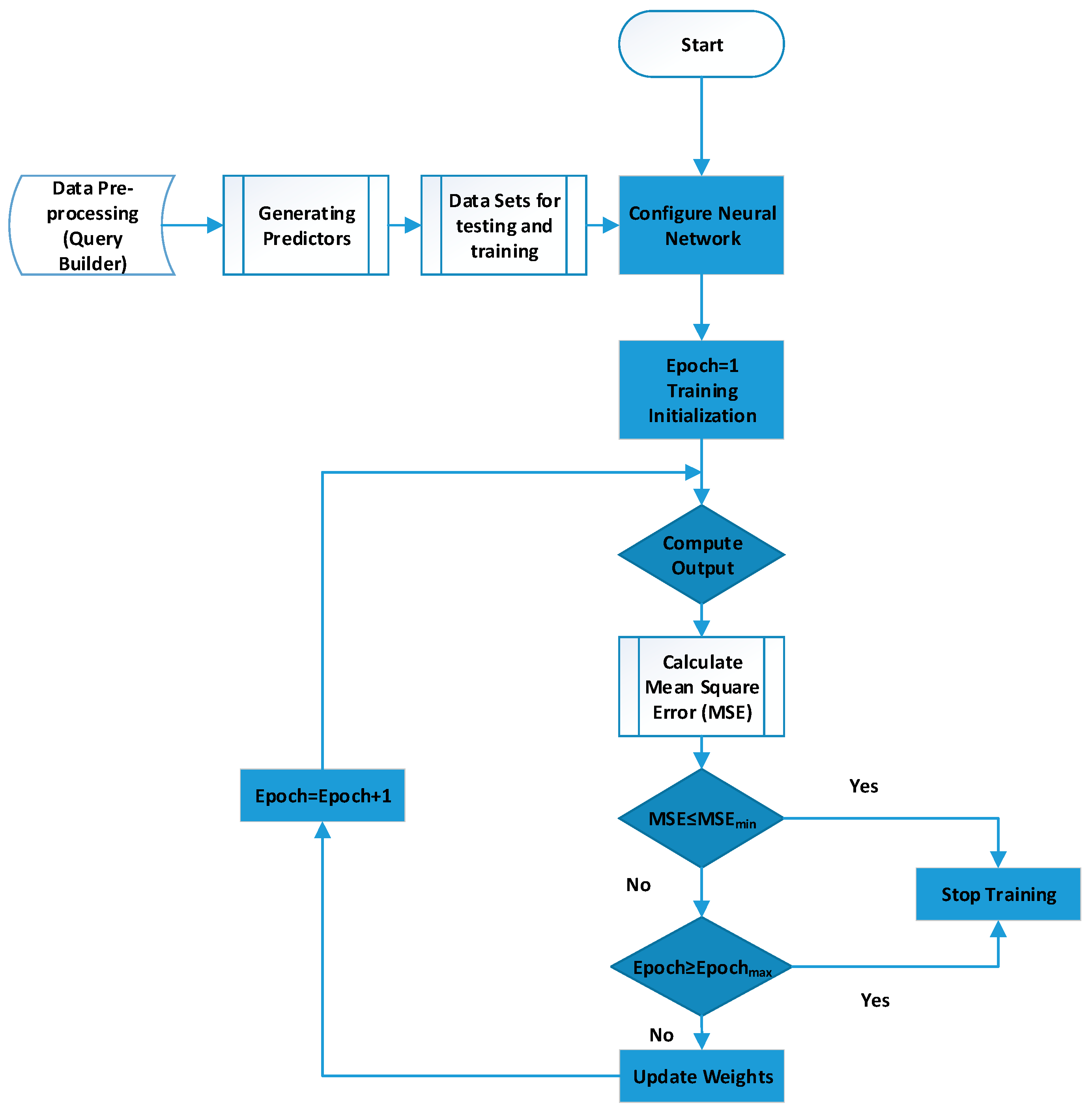
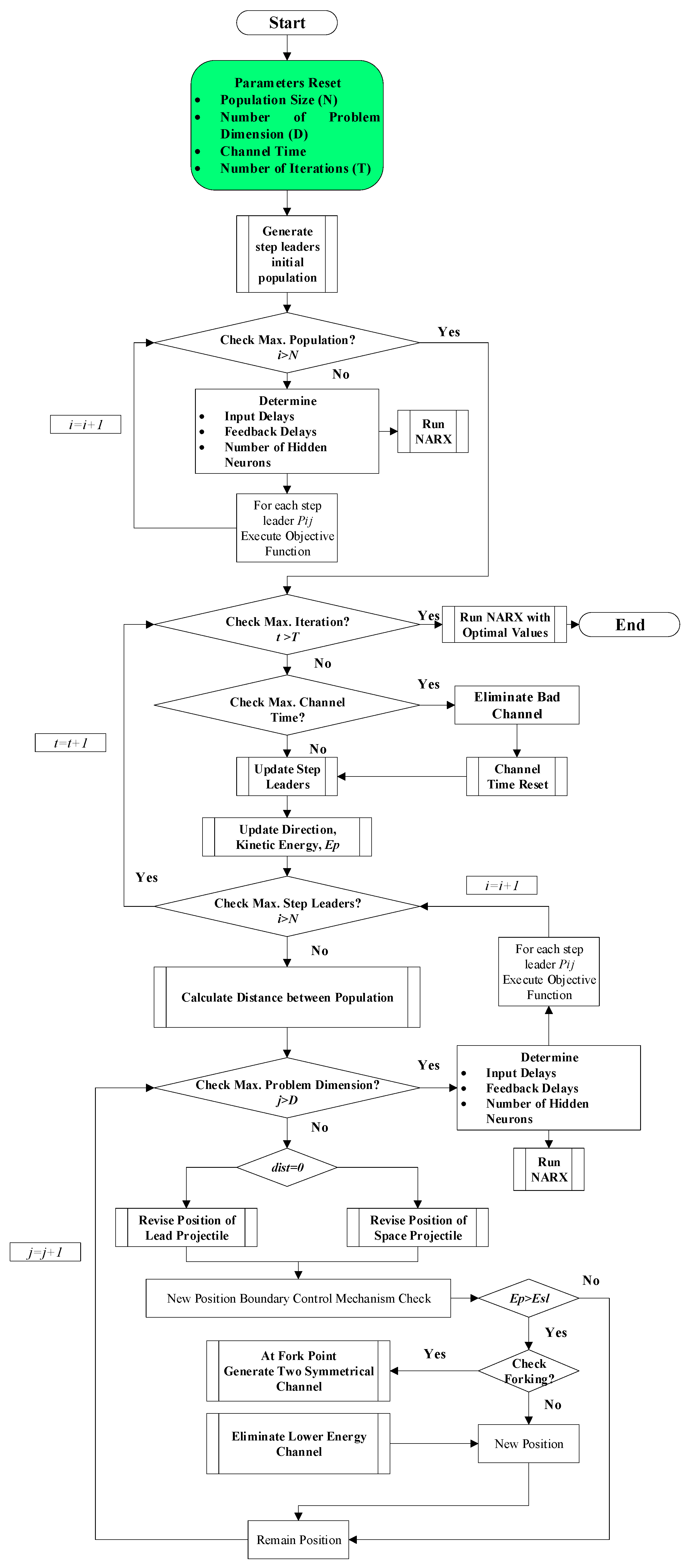
Optimization Algorithm

• Objective

Based on a minimum objective function value, the number of hidden neurons, feedback delays, and input delays are optimized using the equation below.

$$objectivefunction=\min \left[\frac{1}{N}{\displaystyle \sum }_{i=1}^N{\left(I_{es}-I_a\right)}^2\right]$$

(22)

In this case, the actual $I_a$ and estimated $I_{es}$ values are presented for N observations.

• Implementation

Through an iterative process using input and constraints, the objective function is minimized to obtain the best solution. The LSA algorithm is summarized as follows:

• The parameters values are declared, which includes population size, channel time, and number of iterations. Moreover, boundaries are assigned for three-dimensional numbers of hidden neurons, feedback delays, and input delays.
  • 100 iterations are considered with 10-channel time.
  • The hidden nodes range are set from 0–20.
  • Delays are set in range 1–64.
• Step leaders are generated randomly within the bounded range for the number of hidden neurons, feedback delays, and input delays.
• Levenberg–Marquardt is used for training with a logistic sigmoid as an activation function. During training, the objective function is calculated for each step leader.
• Considering all step leaders, the iterative process is initiated to find an optimal solution.
• Considering step leader movement, the bad channel is eliminated and the channel time is resettled.
• Step leaders are estimated based on best and worst performance.
• With revised kinetic energy, Ep the network is retrained and the activation function is re-executed. For each step leader, the objective function is reassessed.
• Ejecting space particles and lead particles.
• In case the energy of space and lead projectiles greater than step leader energy, their direction and position are updated using Equations (18) and (20).
• Re-initialize the updated projectile. The network is retrained and the objective function for lead and space particles is reassessed.
• Two identical channels are formed at the fork point in the case of occurrence of forking. With the least energy, elimination of the channel time is revised.
• All values in the population are updated and the procedure is repeated until the maximum iteration limit.
• The optimal result for the number of hidden neurons, feedback delays, and input delays are utilized in the NARXNN network for the best training and validation.

The Flow chart explaining the LSA optimization algorithm is shown in Figure 8.

4.1.3. Operating Parameters

The data set for five years is segmented into one-year groups including: Date; Month; Year; Hour; Week day; Holiday/Working day; Dry Bulb Temperature; Dew Point Temperature; Humidity; Hourly Load. The data set also include redundant inputs, previous week, and previous day load values. The data is pre-processed to match the size of input neurons. The sub set of each year is used for testing. The processed data is distributed into training, testing, and validation sets. Open loop weights are obtained by training data through Levenberg–Marquardt backpropagation, Bayesian Regularization Backpropagation, and Scaled Conjugate Gradient Backpropagation methods. The process is repeated for a multiple neuron count in order to achieve minimum MAPE criteria. The loop is closed after selecting the Minimum MAPE open loop network. In order to forecast the next 24-h load, the forecasted weather and desired date is fed to the network with one-hour increments. The forecasted output generated is fed back to produce the next 24-h load output. The main parameters of the model include input values, lagged input values, neuron counts in each particular layer, hidden layers, and connection among neurons. The inputs are selected by performing partial and multiple correlation analysis among available variables. The importance of selected predictors is shown in Figure 1. The stepwise selection method is used to find the highest correlated subset. The lag in the input is determined by testing the model form 1-h to 168 h in the case of validation set stopping criteria. The partially best model performance is obtained at a 24-h lag with 10–20 neurons count in the hidden layer. In the case of applied NARX-LSA based criteria, the optimal value for input and feedback delays are 18 and 15, respectively, with 10 hidden neurons. The selected network is fully connected as per NARX definition.

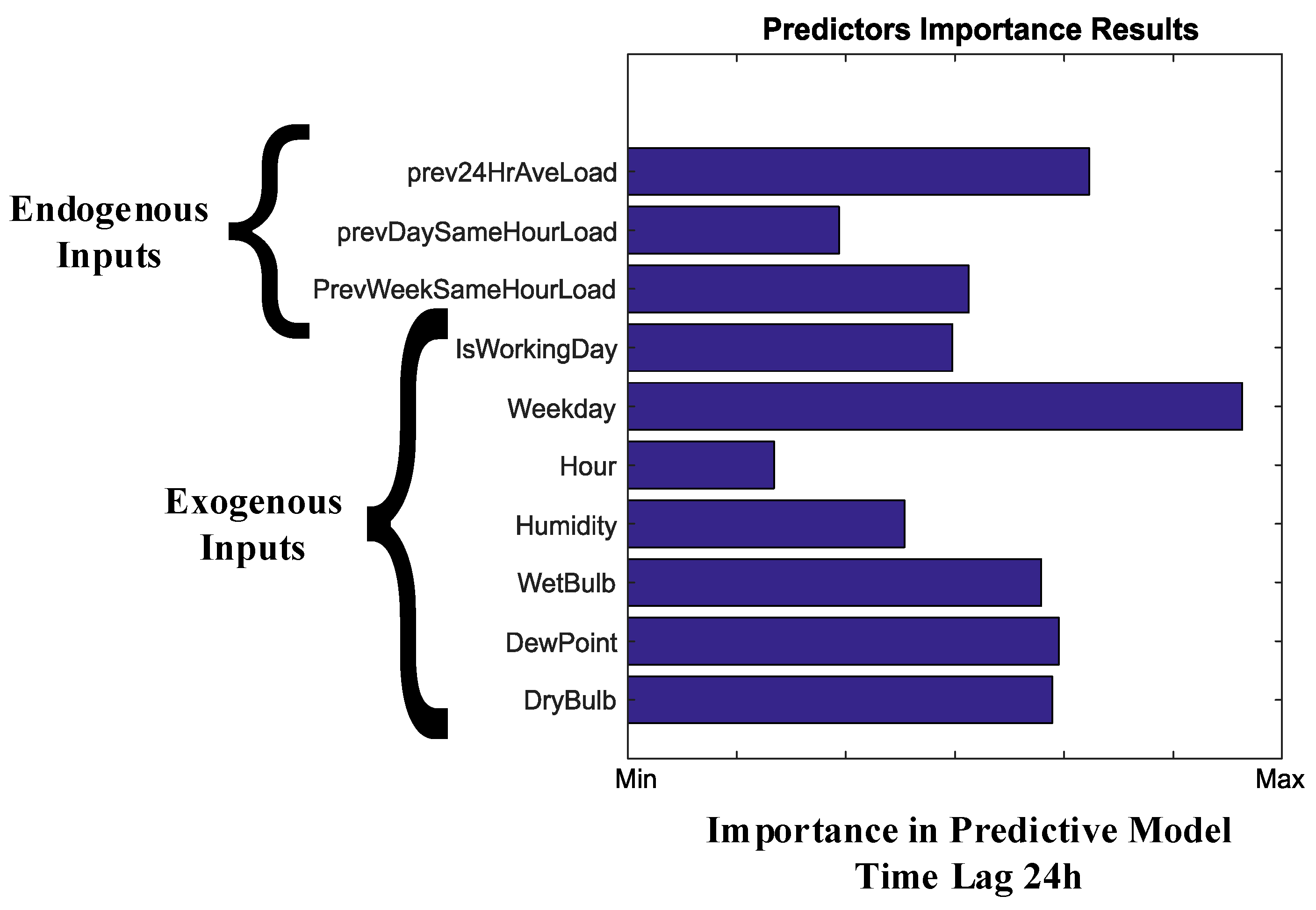
4.1.4. Parameters Selection

A correlation analysis between input predictors and output is performed to maintain a parsimonious nature of the network, i.e., a network that perform more precisely and require minimum inputs. Each input vector is statistically correlated with available residential load, as shown in IESCO data section. The weight given to each predictor in the predictive model is shown Figure 9. The maximum weight is given to inputs connected with weekdays.

The parameters for best NARX network performance with minimum inputs are as follows:

• Input variables are determining the number Input nodes. In the proposed case, 10 variables are taken excluding wet bulb temperature.
• 10 hidden layers have been considered here for the best solution. The number of hidden layers can only be $\ge$1.
• The input nodes are equal to the number of hidden nodes.
• The output nodes are determined by the size of the forecasting period.
• Logistic Sigmoid is used as an activation function, which is mathematically given as:

  $$S\left(t\right)=\frac{1}{1-e^{-t}}$$

  (23)
• The Levenberg–Marquardt backpropagation is used as a learning algorithm, which is mathematically represented as:

  $$x_{i+1}=x_i-{\left(J^{T}J+\partial I\right)}^{-1}{J}^{T}e$$

  (24)

Here, J is the Jacobin matrix, I is the identity matrix, e is to calculate error, $x_{i+1}$ is the iterative input values, and $\partial$ varies between 0–1 and increases only the error in the objective increased during iterations.

The data preparing and pre-processing procedure for NN calibration with proposed methodology is shown in Figure 10. The feature-scaling method is used for normalizing and preprocessing the data. The range is set from [0, 1] and is mathematically represented as:

$$\acute{U}=\frac{U-U_{min}}{U_{max}-U_{min}}$$

(25)

The data set is divided as: 70% for training, 15% for validation, and, for testing the remaining, 15% is used. For improving the network, seasonal dependency of the model is trained with diverse sample sizes varying from two to three years. In the case of the NARX-LSA network, the model training utilized 70% data with 30% data for testing.

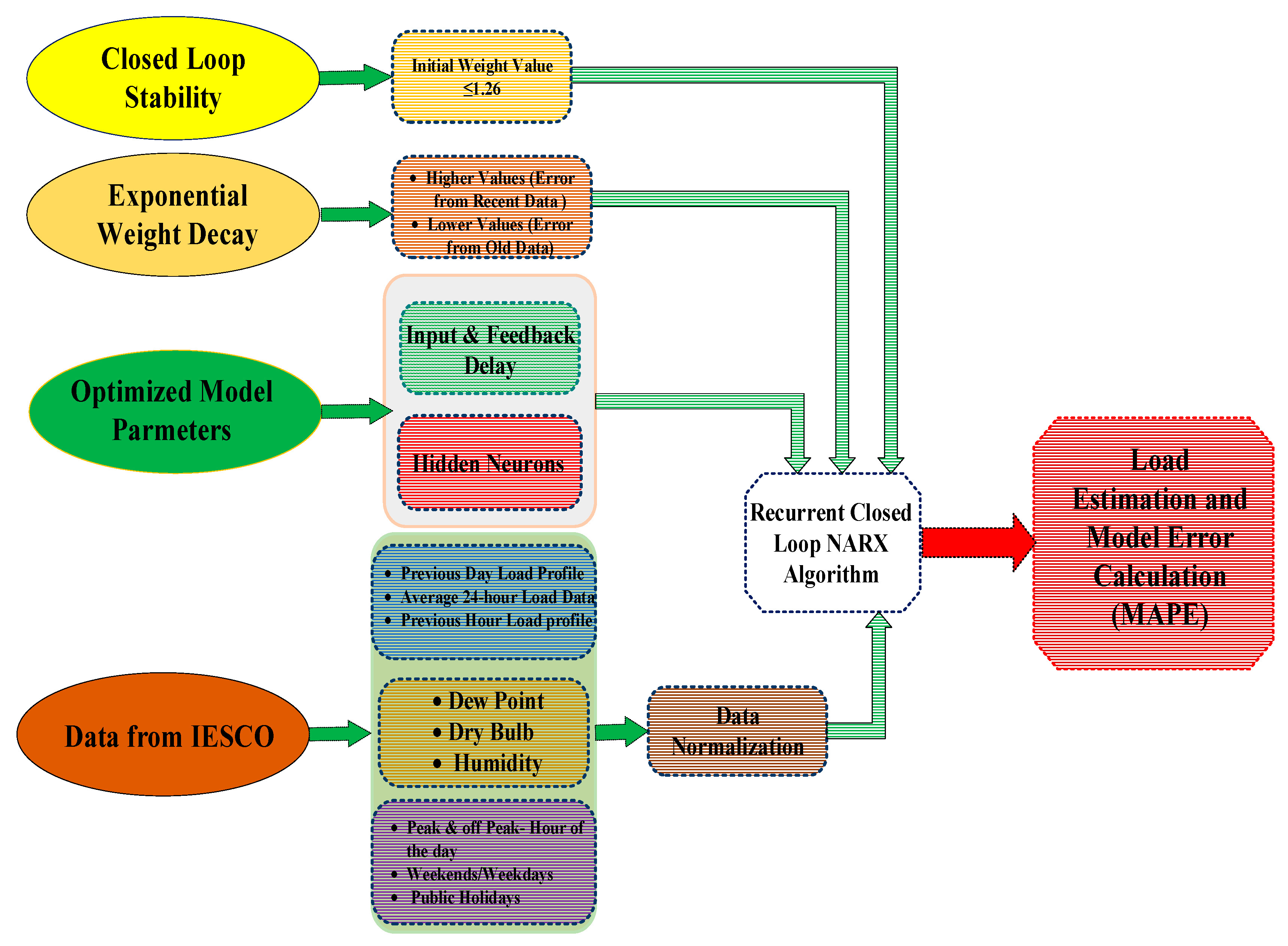
4.1.5. Closed Loop Stability

A proper initial weight selection is pivotal for the network convergence to deal with a closed loop stability issue. A framework is determined in Reference [41] to choose the initial weights for the NARX network. The stability is achieved when the modulus of initial weight fulfill the following.

$${\omega }_{kl}^m\le \frac{4}{\sqrt{KJ}}$$

(26)

where ${\omega }_{kl}^m$ is the initial weight and $K$ and $J$ give the number of neurons in output and hidden layer respectively. For the proposed case, $K=1$ and $J=10$, which gives an initial weight value of $\le 1.26$. The initial weight is taken within the proposed range for resolving the stability issue.

4.1.6. Error Weight Decay

The proposed weight decay function is given as [26]:

$$E\left(\omega \right)=E_o\left(\omega \right)+\frac{1}{2}\mu {\displaystyle \sum }_i{\omega }_i^2$$

(27)

Here, $E\left(\omega \right)$ represents the error function, $\mu$ is the decaying constant, and w is a vector representing bias and weight of the network. For constant error weight, the function for ith iteration is given as:

$$E\left(\omega \right)=\frac{1}{N}{{\displaystyle \sum }}_{i=1}^N{\left(y_i-{\stackrel{\rightharpoonup }{y}}_i\right)}^2$$

(28)

Here. $y$ is the output, $\stackrel{\rightharpoonup }{y}$ is the calculated value of output, and N represents the number of neurons. The above equation is converted for the proposed exponential weight decay and is given below.

$$E\left(\omega \right)=\frac{1}{N}{{\displaystyle \sum }}_{i=1}^N{\left(1-ϵ\right)}^{N-i}{\left(y_i-{\stackrel{\rightharpoonup }{y}}_i\right)}^2$$

(29)

The higher weight values are given to the error generated by recent data and weight values are exponentially reduced for the error generated by historical data.

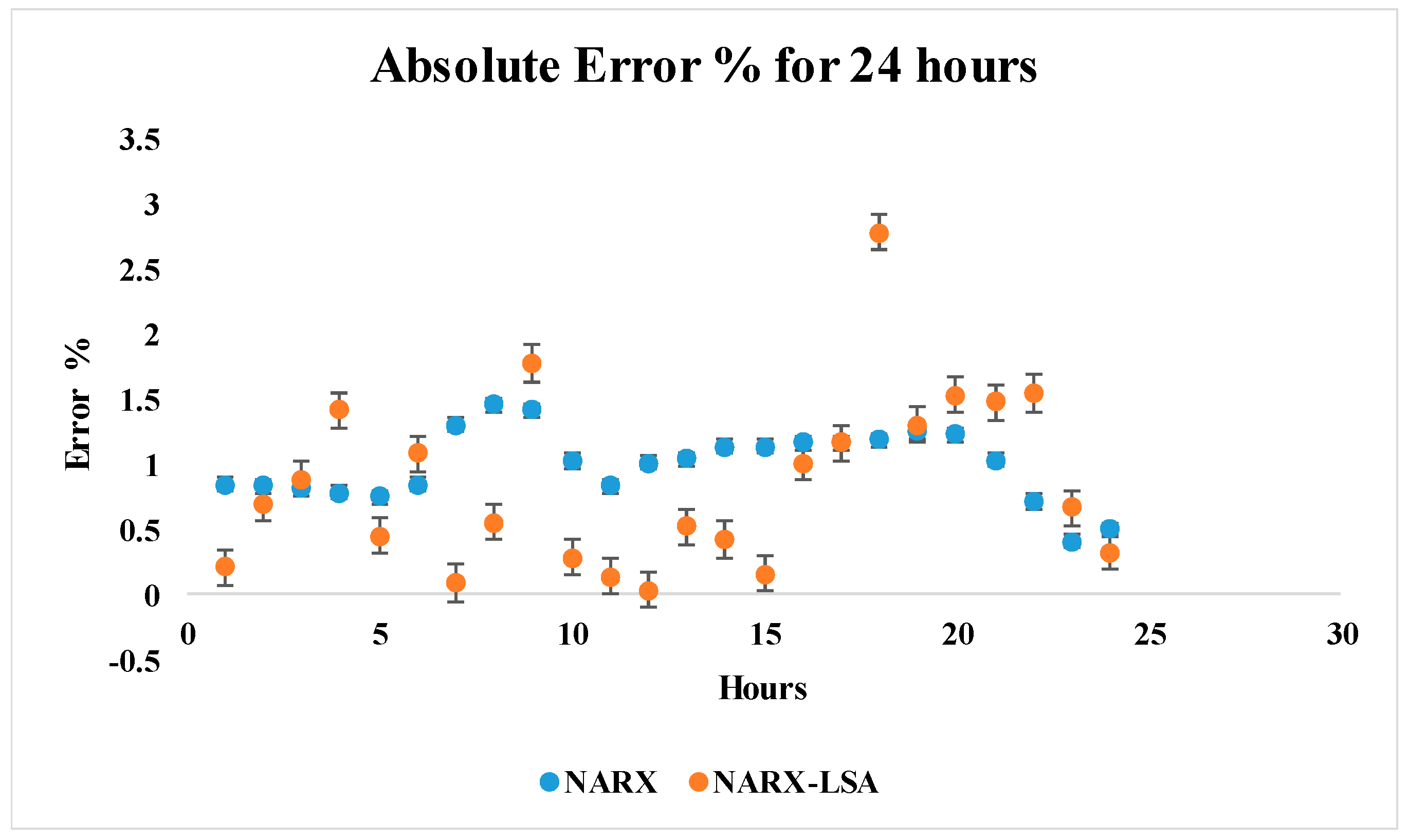
4.1.7. Performance Metrics

The performance is measured by the mean absolute percent error. The error measuring method allows us to determine the accuracy of the utilized forecasting techniques applied to specific time series data. The MAPE and RMSE is defined as:

$$MAPE=\frac{1}{n}{{\displaystyle \sum }}_{i=1}^n\left|E_i\right|\times 100\%$$

(30)

$$RMSE=\frac{1}{n}\sqrt{{{\displaystyle \sum }}_{i=1}^n{\left(L_i^{Actual}-L_i^{Forecast}\right)}^2}$$

(31)

The Error $E_i$ is represented as:

$$E_i=\frac{L_i^{Actual}-L_i^{Forecast}}{L_i^{Actual}}$$

(32)

The performance is measured for all employed techniques, for BRT, fit net NARX close loop case and NARX-LSA-EWD case. The corresponding error is determined as the fit error, which is the residue between the real load value and corresponding output from the validation set. The best network is selected from the minimum error values and is exploited for forecasting. In a closed loop, the actual load known from the past validation set is known. The error is the difference between past output validation data and the forecasted output and is termed as the forecast error.

5. Simulation and Results

ANNs configuration varies structurally depending on parameters used such as counts of hidden layers, a connection strategy among layers, feedback loops, consecutives, and non-consecutiveness layers, feedback within the layers, series-parallel layers etc. Furthermore, important parameters that contribute for best results are:

• Number of Neurons
• Input and Feedback time lags
• Training Data
• Training Algorithm
• Activation function for neurons

The combination of different topologies and parameters provide multiple structural configurations that empowers a particular configuration to work best with diverse data sets. MATLAB 2016 NN Toolbox is used to simulate NARX Network. The Model is run with the IESCO dataset, hourly varying, real-time residential load data is obtained from the IESCO grid operator from 2012–2016. The following network parameters were chosen for simulation purpose: (1) Data is divided into three different periods; multiple runs on each iteration were performed in order to lower the dependency of output on initial conditions. (2) 10-hidden layers a considered with 20 neurons after training the network under define stopping criteria. (3) Levenberg–Marquardt backpropagation algorithm with a logistic sigmoid activation function is used for training.

Based on best MAPE fit on the available data, an open loop NARX model is chosen for a forecasting purpose. The network training is performed in open loop utilizing past available data and the output is used as a next step input for forecasting in a closed-loop. The simulation result comparing actual and predicted load is shown in Figure 11. For a comparative purpose, a FitNet, BRT model is developed in MATLAB along with ARMAX and the state space model in

IBM’s SPSS Package. The results are generated with default FitNet configuration using Levenberg–Marquardt algorithm with 10 hidden layers and 20 trees having the least leaf estimate of 40 are considered for BRT simulation.

SPSS generated the best result for 2,1,8 ARIMA configuration, which is selected by using expert modeler based on the minimum fitness error. The model is then transformed into state space for comparative analysis.

Table 1. Model comparison statistics.

Hour	FitNet Absolute Error%	BRT Absolute Error%	ARMAX Absolute Error%	State Space Absolute Error%	NARX Absolute Error%
1	2.38	2.49	1.15	1.27	0.84
2	2.31	2.71	1.49	1.20	0.83
3	2.13	3.11	0.61	5.18	0.81
4	2.02	2.02	1.49	8.82	0.78
5	2.15	2.06	1.99	1.77	0.75
6	2.57	4.01	1.63	0.97	0.84
7	3.71	6.52	1.85	2.41	1.30
8	4.63	5.83	2.73	6.45	1.45
9	3.91	2.46	2.05	2.08	1.41
10	2.71	1.42	1.02	3.58	1.02
11	2.85	1.46	1.11	2.01	0.83
12	2.45	2.01	1.02	0.78	1.01
13	3.21	2.56	1.10	1.88	1.04
14	3.13	2.51	1.32	2.51	1.13
15	3.24	2.51	1.35	3.83	1.13
16	2.95	2.47	1.89	1.18	1.16
17	3.15	2.06	1.90	3.31	1.16
18	3.12	2.45	1.17	1.80	1.18
19	3.17	4.01	0.98	1.81	1.25
20	3.25	3.92	1.68	1.19	1.22
21	3.24	2.51	1.22	2.21	1.03
22	3.35	2.49	0.78	4.15	0.71
23	2.86	2.13	0.65	3.17	0.41
24	2.75	2.41	0.87	0.85	0.50
Maximum	4.63	6.52	2.73	8.82	1.45
RMSE	9.83	9.75	4.73	8.09	2.61
MAPE%	2.97	2.84	1.43	2.68	0.99

shows the absolute error percentage and the mean absolute percentage error for a 24-h predicted load. The MAPE for the FitNet is 2.97%, for BRT is 2.84%, for the ARMAX model 1.43%, for the state space is 2.68%, and for applied NARX network is 0.99%. A notable improvement is achieved by applied the NARX network with approximately 20% reduction in a forecasting error, as can be seen through a maximum value of an absolute error percentage.

For time series dynamic nonlinear load variations, NARX generates the closest forecast. The advantages and disadvantages of different techniques are given in

Table 2. Advantage and disadvantage for forecasting methods.

Methods	Advantage	Disadvantage
ARIMA/State Space	General class of nonlinear model used for forecasting a regression model and developing a fit. Parametric and autoregressive model used for forecasting applications.	Need Data linearization. Can only work with stationary data. Required complex data preprocessing. Loss of information in residuals for periodic data determined by autocorrelation and partial autocorrelation graphs. Need complex differencing, deflating, and logging techniques for data linearization. Less accuracy with time series data.
Decision Tree	Require less effort for data preparation. Tree performance is not effected by nonlinear data. Easy interpretation.	Required more memory. Difficult to prune. High computational time.
FitNet	Simplicity, improved forecast accuracy. Autocorrelation remains constant over time.	Nonrecurring, constant data set, non-exogenous feedback, solution rely on non-important parameters and less. Dependency on past values. Might over fit. High MAPE values.
NARX-LSA-EWD	Dynamic recurrent network and create memory between inputs and output through lags. Faster convergence. The accuracy is improved by utilizing optimized (LSA) values for the number of neurons, input, and feedback delays. Avoid the possibility of overfitting with an increase in the number of neurons by using the exponential weight decay function. Autocorrelation remains constant over time.	More computational time.

.

Proposed Improvement

The performance efficacy of the NARX network is improved by utilizing LSA optimal solution for hidden neuron, input, and feedback delays. The proposed network performed more accurately with less variance and best fitting. The optimal parameters are utilized to perform training with Levenberg–Marquardt and logistic sigmoid as an activation function.

6. Results & Discussion

The comparative error results for NARX and NARX-LSA is shown in Figure 12 with MAPE in NARX-LSA case of 0.85%. Error distribution is shown in Figure 13 with hourly, weekly, and monthly breakdown for a single house category subjective to follow a similar pattern for other house types. The effect of neurons count on point and mean error can be explored further.

The convergence is obtained at less than 35 epochs when training by using a Levenberg–Marquardt backpropagation algorithm. The error histogram for demonstrating data fitness is shown in Figure 14a and input lag correlation analysis is given in Figure 14b. The network maintained stability as no increase in error is monitored after convergence and there is no overshoot, which can be validated from Figure 15a. The performance metrics between actual and forecasted load is shown by a regression plot in Figure 15b. The closeness of data with fitted regression is shown with value of R = 0.998. The closeness of R values to 1 in the proposed model represents that the data variance is well explained around its mean.

Two training functions, two activation functions, and the error exponential weight decay function is used to test the improvements in the proposed model. The MAPE in each case is analyzed. The result is an average of five runs with an optimal value of a hidden layer neurons, feedback, and input time lags. From the result in

Table 3. Comparative analysis with exponential weight decay.

Training Function	Activation Function	ClosedLoop-NARX-LSA MAPE	Closed Loop-NARX-LSA (Exponential Weight Decay) MAPE
Levenberg-Marquadt	Logistic Sigmoid	0.85	0.821
Levenberg-Marquadt	Hyperbolic Tangent	2.04	2.01
Bayesian Regularization	Logistic Sigmoid	1.22	1.02
Bayesian Regularization	Hyperbolic Tangent	1.11	0.89

, the Levenberg-Marquardt worked well with a logistic sigmoid and Bayesian Regularization performed well with a hyperbolic tangent function. There is little effect on MAPE when using the Levenberg-Marquardt algorithm with an exponential mask. For the Bayesian Regularization case, a notable improvement is observed in an exponential case. The Levenberg-Marquardt with log sigmoid is more susceptible to varying neuron numbers and produce less error across multiple scenarios.

The computational efficiency in terms of training time is better for conventional feedforward and FitNet algorithms. Adding complexity, the training time increased. Average NARX and NARX-LSA took 2–16 s and 20–25 s for training respectively, contrarily FitNet, and feedforward network took 0–9 s for similar neuron variations. The training is performed on an Intel quad core i7 processor with 8 GB storage.

In economic terms, the lower prediction error translates in cost benefit by saving energy cost, which is a resultant obtained by handling power system operations more accurately, which makes the system more reliable. For grid operations like IESCO, the region with continuous economic growth and facing power shortcomings an accurate prediction will help the power company to deal with the load shedding problem more efficiently. The prediction accuracy will help them save cost by not committing expensive independently operated fuel generating units, which can ease the burden on the government by controlling the subsidized amount on the current energy tariff.

Future Consideration

With the proposed electrical load, forecasting technique future research can be realized towards operational cost reduction [42], optimum use of available resources, effective power management, stability analysis [43], and a reliable planning process. The research has been expanded towards forecasting added-peninsular systems in the region. The aim is to test model robustness with highly variable house data and propose feasible energy management plans for the region.

7. Conclusions

In this paper, an autoregressive nonlinear neural network is implemented with external input vectors. The network is originally trained in the open loop by considering available exogenous (climate factors, time factors) and endogenous inputs (historical load) vectors. The network is used in recursive mode with input, hidden, and output layers fully connected. The initial neural weight is determined by operating the network in open loop. The network is fed with forecasted load output in a closed loop. The feedback loop isolated the network from the initial load input, saving the network for utter retaining for each predicted output. Backpropagation Levenberg–Marquardt algorithm with log sigmoid activation function is used for training. The accuracy in terms of MAPE of less than 1% for NARX network validates its effectiveness as compared to conventional feedforward, BRT, and statistical methods (ARMAX, state space). The comparative analysis of statistical and computational methods demonstrated that the proposed NARX network generates least MAPE error. The NARXNN-LSA method features strong robustness, high convergence speed, and high accuracy with no dependency on the model mathematical relationship. The model is further tested by adding a weight decay mask on error weights from old data. The proposed model might have high prospects to be used in a wide range of variable load data, which makes it a useful tool for sustainable energy applications.

References

1. Nengling, T.; Stenzel, J.; Hongxiao, W. Techniques of applying wavelet transform into combined model for short-term load forecasting. Electr. Power Syst. Res. 2006, 76, 525–533. [Google Scholar] [CrossRef]
2. Satish, B.; Swarup, K.S.; Srinivas, S.; Rao, A.H. Effect of temperature on short term load forecasting using an integrated ANN. Electr. Power Syst. Res. 2004, 72, 95–101. [Google Scholar] [CrossRef]
3. Feinberg, E.A.; Genethliou, D. Load Forecasting. Available online: http://www.almozg.narod.ru/bible/lf.pdf (accessed on 9 February 2017).
4. Srivastava, A.K.; Pandey, A.S.; Singh, D. Short-Term Load Forecasting Methods: A Review. Presented at the International Conference on Emerging Trends in Electrical Electronics & Sustainable Energy Systems (ICETEESES), Sultanpur, India, 11–12 March 2016. [Google Scholar]
5. Alfares, H.K.; Nazeeruddin, M. Electric load forecasting: Literature survey and classification of methods. Int. J. Syst. Sci. 2002, 33, 23–34. [Google Scholar] [CrossRef]
6. Raza, M.; Khosravi, A. A review on artificial intelligence based load demand forecasting techniques for smart grid and buildings. Renew. Sustain. Energy Rev. 2015, 50, 1352–1372. [Google Scholar] [CrossRef]
7. Ghayekhloo, M.; Menhaj, M.B.; Ghofrani, M. A hybrid short-term load forecasting with a new data-preprocessing framework. Electr. Power Syst. Res. 2015, 119, 138–148. [Google Scholar] [CrossRef]
8. Metaxiotis, K.; Kagiannas, A.; Askounis, D.; Psarras, J. Artificial intelligence in short term electric load forecasting: A state-of-the-art survey for the researcher. Energy Convers. Manag. 2003, 44, 1525–1534. [Google Scholar] [CrossRef]
9. Hahn, H.; Meyer-Nieberg, S.; Pickl, S. Electric load forecasting methods: Tools for decision making. Eur. J. Oper. Res. 2009, 199, 902–907. [Google Scholar] [CrossRef]
10. Hippert, H.S.; Pedreira, C.E.; Souza, R.C. Neural networks for short-term load forecasting: A review and evaluation. IEEE Trans. Power Syst. 2001, 16, 44–55. [Google Scholar] [CrossRef]
11. Bennett, C.; Stewart, R.A.; Lu, J. Autoregressive with exogenous variables and neural network short-term load forecast models for residential low voltage distribution networks. Energies 2014, 7, 2938–2960. [Google Scholar] [CrossRef]
12. Hernandez, L.; Baladrón, C.; Aguiar, J.M.; Carro, B.; Sanchez-Esguevillas, A.J.; Lloret, J. Short-Term Load Forecasting for Microgrids Based on Artificial Neural Networks. Energies 2013, 6, 1385–1408. [Google Scholar] [CrossRef] [Green Version]
13. Hernandez, L.; Baladron, C.; Aguiar, J.M.; Calavia, L.; Carro, B.; Sanchez-Esguevillas, A.; Sanjuan, J.; Gonzalez, L.; Lloret, J. Improved short-term load forecasting based on two-stage predictions with artificial neural networks in a microgrid environment. Energies 2013, 6, 4489–4507. [Google Scholar] [CrossRef]
14. Fattaheian, S.; Fereidunian, A.; Gholami, H.; Lesani, H. Hour-ahead demand forecasting in smart grid using support vector regression (SVR). Int. Trans. Electr. Energy Syst. 2014, 24, 1650–1663. [Google Scholar] [CrossRef]
15. Mahmoud, T.S.; Habibi, D.; Hassan, M.Y.; Bass, O. Modelling self-optimised short term load forecasting for medium voltage loads using tunning fuzzy systems and Artificial Neural Networks. Energy Convers. Manag. 2015, 106, 1396–1408. [Google Scholar] [CrossRef]
16. Lei, J.; Jin, T.; Hao, J.; Li, F. Short-term load forecasting with clustering–regression model in distributed cluster. Clust. Comput. 2017, 1–11. [Google Scholar] [CrossRef]
17. Buitrago, J.; Abdulaal, A.; Asfour, S. Electric load pattern classification using parameter estimation, clustering and artificial neural networks. Int. J. Power Energy Syst. 2015, 35, 167–174. [Google Scholar] [CrossRef]
18. Abdulaal, A.; Buitrago, J.; Asfour, S. Electric Load Pattern Classification for Demand-side Management Planning: A Hybrid Approach. In Software Engineering and Applications: Advances in Power and Energy Systems; ACTA Press: Marina del Rey, CA, USA, 2015. [Google Scholar]
19. Gajowniczek, K.; Nafkha, R.; Ząbkowski, T. Electricity peak demand classification with artificial neural networks. Ann. Comput. Sci. Inf. Syst. 2017, 11, 307–315. [Google Scholar] [Green Version]
20. Ząbkowski, T.; Gajowniczek, K.; Szupiluk, R. Grade analysis for energy usage patterns segmentation based on smart meter data. In Proceedings of the 2015 IEEE 2nd International Conference on Cybernetics (CYBCONF), Gdynia, Poland, 24–26 June 2015; pp. 234–239. [Google Scholar]
21. Singh, S.; Yassine, A. Big Data Mining of Energy Time Series for Behavioral Analytics and Energy Consumption Forecasting. Energies 2018, 11, 452. [Google Scholar] [CrossRef]
22. Ekonomou, L.; Christodoulou, C.; Mladenov, V. A Short-Term Load Forecasting Method Using Artificial Neural Networks and Wavelet Analysis. Int. J. Power Syst. 2016, 1, 64–68. [Google Scholar]
23. Ekonomou, L.; Oikonomou, D. Application and comparison of several artificial neural networks for forecasting the Hellenic daily electricity demand load. In Proceedings of the 7th WSEAS International Conference on Artificial Intelligence, Knowledge Engineering and Data Bases, Cairo, Egypt, 29–31 December 2008; pp. 67–71. [Google Scholar]
24. Easley, M.; Haney, L.; Paul, J.; Fowler, K.; Wu, H. Deep neural networks for short-term load forecasting in ERCOT system. In Proceedings of the IEEE Texas Power and Energy Conference (TPEC), College Station, TX, USA, 8–9 February 2018. [Google Scholar]
25. Shareef, H.; Ibrahim, A.A.; Mutlag, A.H. Lightning search algorithm. Appl. Soft Comput. 2015, 36, 315–333. [Google Scholar] [CrossRef]
26. Krogh, A.; Moody, J.; Hanson, S.; Hertz, J.A. A simple weight decay can improve generalization. Adv. Neural Inf. Process. Syst. 1995, 4, 950–957. [Google Scholar]
27. Hinton, G.E. Learning translation invariant recognition in a massively parallel networks. In Proceedings of the International Conference on Parallel Architectures and Languages Europe, Eindhoven, The Netherlands, 15–19 June 1987; pp. 1–13. [Google Scholar]
28. Moody, J.E. Note on generalization, regularization and architecture selection in nonlinear learning systems. In Proceedings of the Neural Networks for Signal Processing—1991 IEEE Workshop, Princeton, NJ, USA, 30 September–1 October 1991; pp. 1–10. [Google Scholar]
29. User, S. IESCO Annual Performance Reports. Daily, Monthly and Quarterly Data. Available online: http://www.iesco.com.pk/index.php/customer-services/dailymonthly-yearly-data (accessed on 20 January 2018).
30. 2005 ASHRAE Handbook. Design Conditions for ISLAMABAD (CIV/MIL), Pakistan. 2005. Available online: http://cms.ashrae.biz/weatherdata/STATIONS/415710_s.pdf (accessed on 1 February 2018).
31. AAI-hamadi, H.; Soliman, S.A. Long term/Mid term electric load forecasting based on short-term correlation and annual growth. Electr. Power Syst. Res. 2005, 74, 353–361. [Google Scholar] [CrossRef]
32. Pappas, S.S.; Ekonomou, L.; Karamousantas, D.C.; Chatzarakis, G.E.; Katsikas, S.K.; Liatsis, P. Electricity demand loads modeling using autoregressive moving average (arma) models. Energy 2008, 33, 1353–1360. [Google Scholar] [CrossRef]
33. Lee, C.; Ko, C. Short-term load forecasting using lifting scheme and ARIMA models. Expert Syst. Appl. 2011, 38, 5902–5911. [Google Scholar] [CrossRef]
34. Breiman, L. Bagging Predictors; Department of Statistics University of California: Berkeley, CA, USA, 1994. [Google Scholar]
35. Kalaitzakis, K.; Stavrakakis, G.S.; Anagnostakis, E.M. Short-term load forecasting based on artificial neural networks parallel implementation. Electr. Power Syst. Res. 2002, 63, 185–196. [Google Scholar] [CrossRef]
36. Senjyu, T.; Takara, H.; Uezato, K.; Funabashi, T. One hour load orecasting using Nueral network. IEEE Trans. Power Syst. 2002, l7, 113–118. [Google Scholar] [CrossRef]
37. Ning, Y.; Liu, Y.; Zhang, H.; Ji, Q. Comparison of different BP neural network models for short-term load forecasting. In Proceedings of the 2010 IEEE International Conference on Intelligent Computing and Intelligent Systems, Xiamen, China, 29–31 October 2010; Volume 3, pp. 433–438. [Google Scholar]
38. Haykin, S. Neural Networks-A comprehensive foundation. In Neural Network A—Comperhensice Foundation, 2nd ed.; Prentice Hall: Upper Saddle River, NJ, USA, 1999. [Google Scholar]
39. Upadhyay, K.G.; Tripathi, M.M.; Singh, S.N. An Approach to Short Term Load Forecasting using Market Price Signal. In Proceedings of the International Conference on Distribution (CIRED), Vienna, Austria, 21–24 May 2007. [Google Scholar]
40. Venturini, M. Simulation of compressor transient behavior through recurrent neural network models. J. Turbomach 2006, 128, 444–454. [Google Scholar] [CrossRef]
41. Irigoyen, E.; Pinzolas, M. Numerical bounds to assure initial local stability of narx multilayer perceptrons and radial basis functions. Neurocomputing 2008, 72, 539–547. [Google Scholar] [CrossRef]
42. Abbas, F.; Habib, S.; Feng, D.; Yan, Z. Optimizing Generation Capacities Incorporating Renewable Energy with Storage Systems Using Genetic Algorithms. Electronics 2018, 7, 100. [Google Scholar] [CrossRef]
43. Rasool, A.; Yan, X.; Rasool, H.; Guo, H.; Asif, M. VSG Stability and Coordination Enhancement under Emergency Condition. Electronics 2018, 7, 202. [Google Scholar] [CrossRef]
Figure 1. Residential load pattern for different house categories.
Electronics 07 00432 g001
Figure 2. Load variations vs. weather data.
Electronics 07 00432 g002
Figure 3. Pearson correlation of input parameters.
Electronics 07 00432 g003
Figure 4. ANN Basic Architecture.
Electronics 07 00432 g004
Figure 5. ANN Process Stages.
Electronics 07 00432 g005
Figure 6. NARX architecture.
Electronics 07 00432 g006
Figure 7. Parameter selection with the stopping criteria method.
Electronics 07 00432 g007
Figure 8. NARX-LSA flow chart.
Electronics 07 00432 g008
Figure 9. ANN inputs importance in predictive model.
Electronics 07 00432 g009
Figure 10. Proposed network flowchart.
Electronics 07 00432 g010
Figure 11. (a) Actual load vs model prediction (1-Kanal), (b) actual load vs model prediction (10-Marla), (c) actual load Vs model prediction (7-Marla), (d) actual load Vs model prediction (5-Marla).
Electronics 07 00432 g011
Figure 12. Error analysis NARX, NARX-LSA.
Electronics 07 00432 g012
Figure 13. (a) Hourly error distribution, (b) weekly error distribution, (c) monthly error distribution, and (d) mean error distribution.
Electronics 07 00432 g013
Figure 14. (a) Error histogram and (b) error auto correlation with lag inputs.
Electronics 07 00432 g014
Figure 15. (a) Model performance validation and (b) model regression plot.
Electronics 07 00432 g015