A Fast Global Flight Path Planning Algorithm Based on Space Circumscription and Sparse Visibility Graph for Unmanned Aerial Vehicle

Abstract

This paper proposes a new flight path planning algorithm that finds collision-free, optimal/near-optimal and flyable paths for unmanned aerial vehicles (UAVs) in three-dimensional (3D) environments with fixed obstacles. The proposed algorithm significantly reduces pathfinding computing time without significantly degrading path lengths by using space circumscription and a sparse visibility graph in the pathfinding process. We devise a novel method by exploiting the information about obstacle geometry to circumscribe the search space in the form of a half cylinder from which a working path for UAV can be computed without sacrificing the guarantees on near-optimality and speed. Furthermore, we generate a sparse visibility graph from the circumscribed space and find the initial path, which is subsequently optimized. The proposed algorithm effectively resolves the efficiency and optimality trade-off by searching the path only from the high priority circumscribed space of a map. The simulation results obtained from various maps, and comparison with the existing methods show the effectiveness of the proposed algorithm and verify the aforementioned claims.

1. Introduction

Unmanned Aerial Vehicles (UAVs) are becoming increasingly popular due to their ability to operate autonomously even in those areas that are difficult to reach, such as mountains, deserts, and forests for performing a variety of tasks. Nowadays, UAVs being inexpensive, lightweight, and with low and super low-altitude flights capabilities have demonstrated their usefulness in a wide-range of both civilian and military applications. UAV technology continues to advance, driven by both military and civilian investments. According to the Teal Group’s forecast of the rapidly growing global UAV market, annual spending on UAVs including both military and civilian applications, will be more than US $12 billion by 2024 [1]. Technological developments, such as processing speed of computers, sensors, artificial intelligence, and computer vision based algorithms have enabled UAVs to conduct a much wider range of practical applications with ease that otherwise would be done at higher costs and times.

The commercial real-world applications of UAVs, such as vaccine distribution [2], vegetable inspection [3], industrial applications [4], sensing of large areas [5], aerial forest fire detection [6], traffic monitoring [7], scientific research data collection [8], disaster assessment and management [9], rust detection of steel bridges [10], and ocean exploration missions [11], among others, are more attractive than military applications. Meanwhile, the coming generation of UAVs will introduce some unique capabilities that might eventually reshape the future of war around the world [12]. In most of the applications, a UAV needs the ability to reach a target location quickly while avoiding various obstacles it may find along the way. However, without human control, UAV usage imposes several challenges that need to be resolved, and one of those challenges is finding the optimal, collision-free, and computationally efficient flight path between source and target locations in 3D environments. Due to the extensive use of UAVs in many fields, the problem of pathfinding for UAVs has been a very active area of research, especially during the last decade.

Path planning is a method to obtain the most viable path between source and target locations while preventing the collision with the underlying environment, and at the same time satisfying certain optimization constraints, such as time, distance and energy consumption [13]. Path planning is an NP-hard optimization problem that can be solved in deterministic and non-deterministic ways. Generally, path planning problems are divided into two major categories, global and local path planning. In global path planning, the path searching is carried out in a known environment. In contrast, local path planning is relatively complex because the environment can be completely or partially unknown. Considering UAV missions, pathfinding problems are of two types; namely, multi-agent and single-agent pathfinding. In multi-agent pathfinding, a team of UAVs search for their destinations simultaneously unlike the single-agent variant in which one UAV does so. The pathfinding process usually starts with exploring a graph from a starting location and continues until the target location is reached. The performance of any pathfinding algorithm is usually based on the selection of highly relevant nodes and edges from the provided graph that result in an optimal solution with less computing overheads. In this paper, our focus is on the single-agent global path planning problem and our aim is to reduce the overall time required for computing an optimal or near-optimal path.

Several global path planning algorithms have been proposed for enhancing UAV autonomy in an airspace for various missions [14,15,16,17,18,19,20,21,22,23,24,25,26,27]. The pathfinding process is mainly comprised of three key-elements; setting up a suitable environment (e.g., a graph representation of an environment), a search algorithm that explores the graph, and a heuristic function (e.g., distance and energy, etc.) that guides the search. Accurate terrain representation with detailed information is necessary to obtain a natural-looking path. Cell decomposition [28], roadmap [29], and potential field [30] are well-known environment modelling approaches based on configuration space (C-space). Search algorithm explores the terrain from start to the target locations for finding a feasible or optimal path. There exists a series of well-known graph search algorithms developed from 1959 to date, such as Dijkstra [31] and greedy best-first-search [32] which are known as the earliest graph search-based shortest pathfinding algorithms. However, A* algorithm [33] is considered as the de-facto standard, and it is the most widely used shortest path search algorithm. An independent study [34] proved that A* algorithm is faster and more efficient than Dijkstra’s algorithm and its variants. Apart from these well-known algorithms, many variants of A* algorithm, such as Theta* [35], IDA* [36], LPA* [37], Lazy-theta* [38] and D*-Lite [39] can almost always find an optimal or near-optimal path. Most graph-based pathfinding algorithms use a heuristic function that guides the search which can be either Euclidean distance or energy estimates [40]. Algfoor et al. [41] study has provided a detailed survey about path planning techniques for robotics.

Most of the existing pathfinding algorithms for UAVs do not provide thorough insight into search space circumscription, particularly regarding the trade-off between optimality and speed in large and complex 3D environments. Current pathfinding algorithms focus on building better heuristics at the expense of memory overheads. Many algorithms sacrifice optimality for speed. Few offer near-optimal paths or time performance guarantees, most provide only shortest paths, risking time performance degradation. However, in many practical UAV applications, trade-off on any of the given metrics is not acceptable. Therefore, it is mandatory to constrain the path searches only to high priority space during pathfinding to effectively resolve the efficiency and optimality trade-off. Various approaches have been proposed to speed-up the path computations, such as hierarchical abstractions [42,43,44], symmetry breaking [45,46], jump point search [47,48,49,50], sub-goal graphs [51], compressed path databases [52,53], accurate heuristics [54], swamp hierarchies [55], pruning dominant states [56], influence-aware pathfinders [57], and constraints-aware navigation (CAN) [58]. Despite the success of such enhancements, in most cases, either many locations of the maps are searched needlessly, or path length degrades. In unrealistic cases, the worst-case running time of most algorithms increase exponentially, and extensive pre- and post-processing are needed to obtain the final path.

Recently, some studies have focused on the problem of reducing the time complexity of pathfinding by considering the obstacles that are on the straight line path between the source and target locations or their extensions in the pathfinding process [59,60]. However, these methods are subject to very high computational complexity and return non-taut paths if large numbers of obstacles are lying on the straight line path. Therefore, such methods are prone to either inefficient paths or need additional computation in finding the feasible path. To overcome the aforementioned limitations, this study proposes a new flight path planning algorithm that reduces pathfinding computing time significantly without significantly degrading path lengths by using space circumscription and sparse visibility graph in 3D environments with fixed convex obstacles. The essence of the proposed approach is to search only the desired region and to avoid unwanted regions by exploiting the obstacle geometry to find good quality paths.

The remainder of this paper is organized as follows; Section 2 explains the background and related work regarding well-known path planning algorithms. Section 3 presents the proposed global flight path planning algorithm and explains its principal steps. Section 4 discusses the experiments and results. Finally, conclusions and future directions are offered in Section 5.

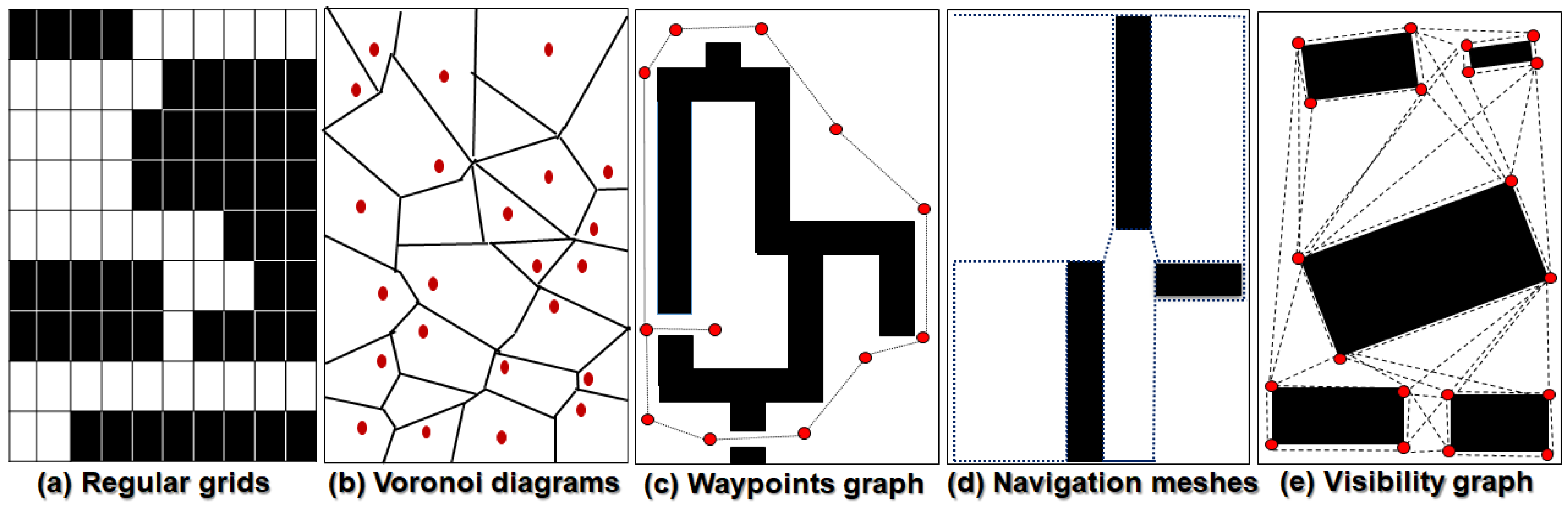
2. Background and Related Work

This section presents the background and related work regarding the environment representation techniques used for UAV path planning, path optimization algorithms and obstacle geometry preserving UAV path planning methods. The primary step of global path planning is to represent the world space with appropriate geometrical shapes. Environment representation is highly related to a path search algorithm because some path search algorithms only do well when they are jointly used with a specific environment representation. A detailed overview of the performance of different environment representations jointly used with various search algorithms is presented in [61]. There are plenty of methods in the existing literature to represent the UAV operating environment. These methods are broadly classified into three categories: cell decomposition (CD), roadmap (RM), and potential fields (PF). A detailed survey regarding environment modelling techniques was given by Kim et al. [62]. Each method varies regarding the degree of computational complexity, accuracy of environment representation, and solution quality. For instance, the main weakness of the CD-based methods is poor solution quality when the cell sizes are too coarse. On the other hand, they are prone to very high space and time complexity if the cells are too fine. Meanwhile, PF-based methods suffer from the local minima problem and degrade the solution quality. A pictorial overview of the most widely used environment representation methods is given in Figure 1.

After representing the UAV operating environment in the form of a graph, a search algorithm is employed to explore the graph for shortest pathfinding. Due to the extensive use of UAVs in many fields, several attempts have been made to find the optimal or feasible path with less time complexity. The path planning algorithms, such as firefly algorithm (FA) [63], differential evolution (DE) [64], genetic algorithms (GA) [65], ant colony optimization (ACO) [66], particle swarm optimization (PSO) [67], artificial bee colony (ABC) [68], fuzzy logic (FL) [69], gravitational search algorithm (GSA) [70], central force optimization (CFO) [71], simulated annealing (SA) [72] and their improved versions, are used in global path planning. Each algorithm has its own strength over others in terms of robustness, ease of implementation, simplicity, usability, scalability, convergence, and environment representation. Due to simplicity and effectiveness, PSO, GA, ACO, ABC, and FA are the most appealing to solve the global optimization problems. However, in some cases, GA and PSO algorithms fall into premature convergence which results in poor solution quality. DE algorithms are plausible because they require only few control parameters. CFO algorithms have demonstrated their effectiveness in finding the feasible or optimal path under complicated constraints. In some cases, multiple algorithms have been jointly used to find the path for UAV [73]. A comprehensive survey regarding four fundamental path planning families was provided by Yang Liang et al. [74].

A geometrical path planning method that enables a UAV to find a feasible path in 3D complex environments with less time complexity was offered by [75]. The proposed algorithm models the environment with height reduction to resolve the conflict between accuracy of environment modelling and path finding efficiency. Unfortunately, the proposed method does not constrain the path search in the remaining UAV operating area after height reduction which can greatly affect the efficiency of pathfinding in large and complex environments. Liang Hu et al. [76] proposed an incremental path planning algorithm to solve the optimal pathfinding problem with least computation cost considering the environmental and UAV constraints. The proposed algorithm is rapid and reduces the path set to only four paths of desired quality with less time complexity. However, the authors make no attempt to reduce the search space size to find the candidate solution efficiently. A general-purpose strategy to improve time complexity of pathfinding by utilizing multi-scale information of the environments was provided by the authors in [77], and this seems to be a reliable and practical solution. A related review of the literature on improving the runtime search of the pathfinding process was introduced by [78] using sparse A* search (SAS). They draw attention to construct the search space with a reasonable number of nodes via a random function to compute an initial path which is then further optimized. The main weakness of their study is that they make no attempt to reduce the UAV path planning area and consider only few geometric constraints while deploying random nodes. Wang Zhu et al. [79] proposed an enhanced SAS using Dubins path estimation that can significantly reduce path planning time while preserving path accuracy by expanding only a few nodes.

Zhang Kun et al. [80] proposed an improved heuristic algorithm based on SAS considering the UAV flight constraints to find a feasible path efficiently. Sikha Hota and Debasish Ghose [81] proposed a geometric approach for optimal path planning in 3D space considering UAV minimum turn radius. The proposed approach is efficient and reliable in finding a working path even from complex 3D configuration spaces. Evis Plaku et al. [82] proposed a novel over-segmentation method to produce an overlay of the free space into a set of connected regions. The proposed approach yields collision-free and optimal paths with less time complexity. However, the proposed approach does not consider the information about narrow passages, sharp turns, and terrain difficulty that may degrade the algorithm performance in complex 3D environments. An even greater source of concern is to identify the irrelevant areas of the terrain to prune if they cannot contribute to optimal or near-optimal solutions to improve both accuracy and efficiency of pathfinding [83].

A number of studies have explored a closely related method used for UAV pathfinding with reduced time complexity, the approximation with visibility line algorithm (ApVL) [84], and the related bounded space algorithm [85]. The ApVL algorithm [84] is an extension of the BLOVL algorithm [60] and it is a promising method for approximate shortest pathfinding for UAVs in urban environments. The proposed method reduces the number of obstacles in pathfinding process (e.g., only consider the straight-line path obstacles), and generates visibility graphs from selected obstacles to find the approximate shortest path incrementally. The proposed algorithm has very high time complexity. Furthermore, the proposed algorithm either produces an inefficient path or requires additional computations to find a collision-free path. In some scenarios, the proposed algorithm even fails to find a valid path due to numerous nearby obstacles. It has been suggested [85] that time complexity of UAV path planning can be significantly reduced by restricting the search space only to a region of interest and this seems to be a reliable solution. The proposed method limits the search space and generates the visibility graph with equi-spaced vertical planes to find collision-free paths. However, the proposed method does not consider the suitability of the first bounded space from a pathfinding point of view and generates a dense visibility graph which increases the time cost.

Sample-based methods, such as rapidly exploring random trees (RRTs) [86], probabilistic roadmaps (PRMs) [87] and their improved versions, are capable of generating near-optimal global solution in a short time. Due to the conceptual simplicity these algorithms have demonstrated their effectiveness in solving single-query and real-time path planning problems. RRT algorithm and its variants such as Transition-based RRT (T-RRT) [88], Informed RRT* [89], Anytime T-RRT (AT-RRT) [90] and RRT-connect [91] are probabilistically complete. Most of the RRT based algorithms have slow convergence rate in high dimensional spaces and they often sacrifice optimality for speed. Karaman and Frazzoli [92] proposed an extended version of the RRT, named RRT*. The proposed solution has better convergence rate than RRT and it finds a near-optimal path through postprocessing. However, the constraints. such as high memory consumption, slow convergence rate, exploration of the whole space and pre-mature convergence by discarding the beneficial samples, make it unsuitable for complex problems. Nasir et al. [93] proposed a variant of RRT* called RRT*-Smart which has better convergence rate than the original RRT* by using the path optimization techniques and intelligent sampling. However, the key limitations of the proposed solution are the high sensitivity to the environment map, large number of iterations and extensive storage requirements. Noreen et al. [94] provided the detailed comparison between three RRT-based methods. A recent study by Iram et a. [95] presents the closely related method to our study based on RRT* named RRT*-AB to find an optimal path. The proposed solution has significant improvements over the conventional RRT* methods. However, the proposed approach is prone to the time performance overheads due to the extensive rewiring operations and near-neighbour search during path length optimization. Therefore, optimal/near-optimal paths produced by the existing algorithms have high computational overheads. Accordingly, an obstacle’s geometry and reduced space feasibility analysis have not been jointly considered to obtain better solution quality with less time complexity.

The contributions of this research in the field of UAV global flight path planning can be summarized as follows: (i) it proposes a new flight path planning algorithm based on space circumscription and a sparse visibility graph that has potentials to obtain the optimal or near-optimal path with less time complexity; (ii) it introduces a novel space circumscription method in which a full 3D map is transformed into a circumscribed half cylinder space with path guarantees; (iii) it determines the feasibility of the circumscribed half cylinder space for good quality pathfinding considering multicriteria such as ratio of occupied spaces, dominance of the obstacles, diversity of obstacle avoidance options and ratio of overlapped obstacles; (iv) it expands the circumscribed half cylinder space to next space by exploiting the nearby obstacle geometry if the first circumscribed space fails to offer potential for good quality paths; (v) it generates a sparse visibility graph from the circumscribed space and finds the initial path, which is further optimized by adding more nodes around the initial path nodes.

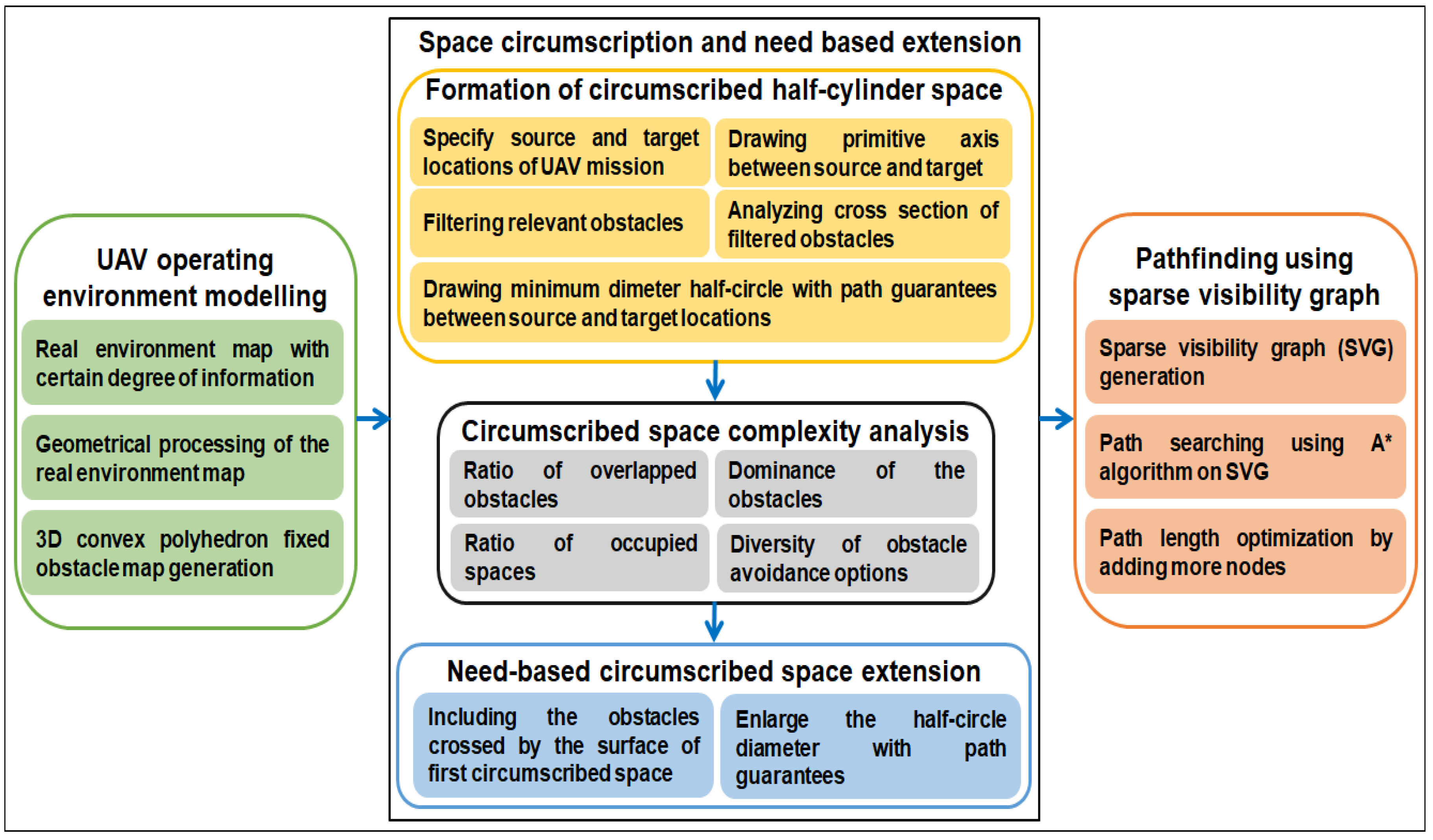
3. The Proposed Global Flight Path Planning Algorithm

A space circumscription and sparse visibility graph-based path planning algorithm is necessary to account for the time performance issues stemming from the needless path searches on low-priority spaces of obstacle-rich environments. This algorithm not only reduces time complexity of pathfinding, it also improves path length by exploiting the information about obstacle geometry. The proposed algorithm constrains the path search only to the circumscribed space and safely discards the low-priority spaces from the map that possibly cannot contribute to an optimal or near-optimal path to speedup pathfinding computations. The proposed algorithm effectively resolves the efficiency and accuracy trade-off in UAV pathfinding. This section presents the conceptual overview of the proposed path planning algorithm and outlines its procedural steps. Figure 2 shows the conceptual overview of our proposed global flight path planning algorithm.

To find a path between two locations, source u and target v for UAV while avoiding the obstacles present in the operating environment, the following seven principal concepts are introduced: (1) modelling of the UAV operating environment from the real environment map; (2) formation of the circumscribed half cylinder space; (3) multicriteria-based circumscribed half cylinder space complexity analysis; (4) need based extension of the circumscribed half cylinder space; (5) sparse visibility graph generation; (6) initial pathfinding using $A^{*}$ algorithm; and (7) path length optimization by adding more nodes around the initial path nodes. This approach is chosen to lower the overall time required to compute an optimal or near-optimal path by exploiting the geometry of the obstacles. Brief details of the principal components with equations and procedures are as follows.

3.1. Modelling of the UAV Operating Environment

The first step of path planning is to model the UAV operating environment with abstract geometrical shapes from a real environment map. It is a way to classify the free ($X_{free}$) and obstacle regions ($X_{obstacles}$), and obstacles can be represented with geometrical shapes, such as cylinders, cubes, polygons and prisms etc. However, in real environments, the shapes and sizes of the objects are not uniform and do not pose an exact geometrical figure, but uneven shaped objects are modelled with their closely resembled geometrical shapes. In this paper, we model the obstacles present in the UAV operating area with 3D convex polyhedrons having six faces. The base height of every obstacle is zero. We process the digital map elevation data according to digital terrain elevation data standard and calculate the convex hull to generate the set of convex obstacles. After geometrical processing of the real environment map a 3D convex polyhedron fixed obstacles map is obtained in the form of a 3D co-ordinate space. Any point p in the modelled environment can be represented with their co-ordinates, $p=(x,y,z)$. The source location is represented with a point u, where $u=(x_s,y_s,z_s)$ and destination is represented with a point v, where $v=(x_t,y_t,z_t)$. Considering the UAV environment representation and pathfinding in 3D environments, the objective of the proposed path planning algorithm is to reduce the computing time of pathfinding without impacting the solution quality while finding a collision-free path W from u to v. The path nodes set (W) can be defined as, $W\in X_{free}$ and $W\cap X_{obstacles}=\varnothing$. In this work, for the path planning problem, the functional model between u and v for two objective optimization is as follows:

$$\left\{\begin{array}{c}W=[u=w_1,w_2,w_3,\cdots ,w_n,w_{n+1}=v]\hfill \\ Minimize{f}_1\left(W\right)=Length\left(W\right)\hfill \\ Minimize{f}_2\left(W\right)=ComputingTime\left(W\right)\hfill \end{array}\right.$$

The proposed algorithm effectively resolves the two conflicting objectives by making use of the obstacles’ geometry information, and UAV is assumed to be a single point.

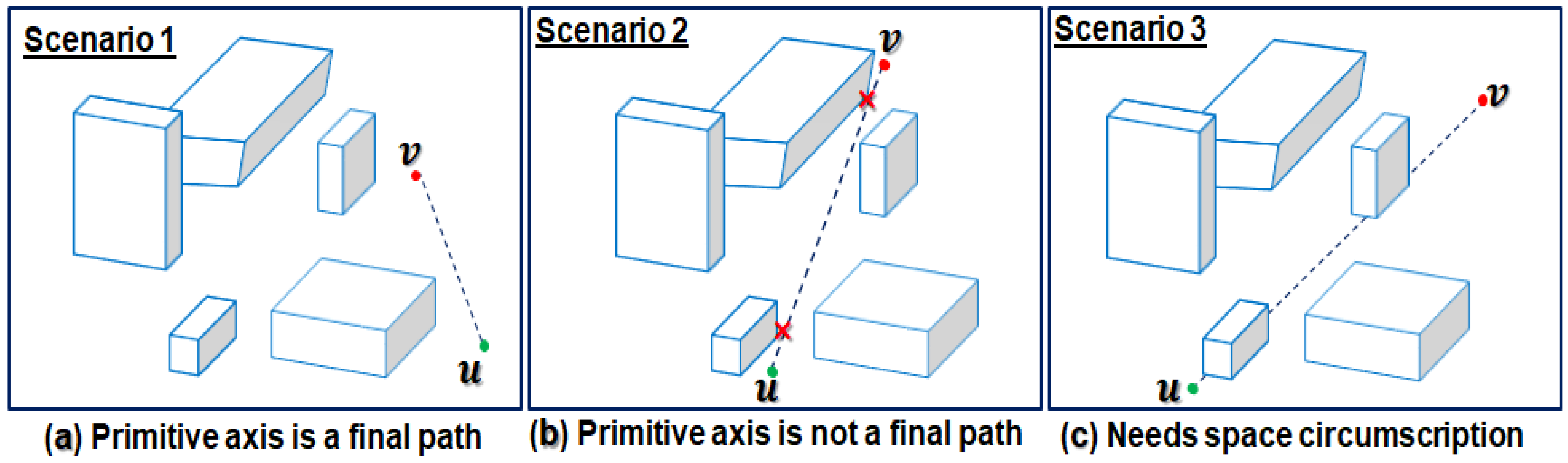
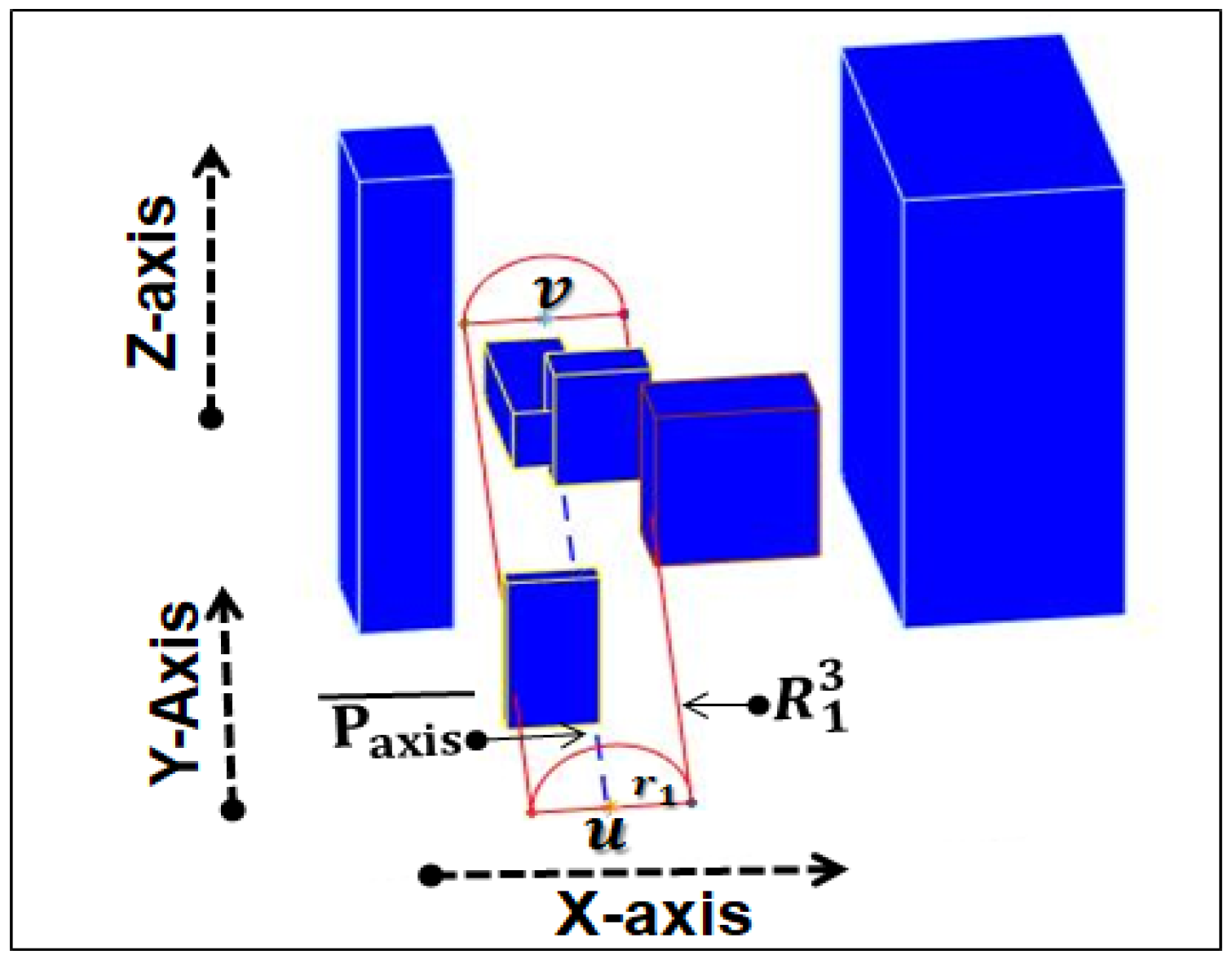
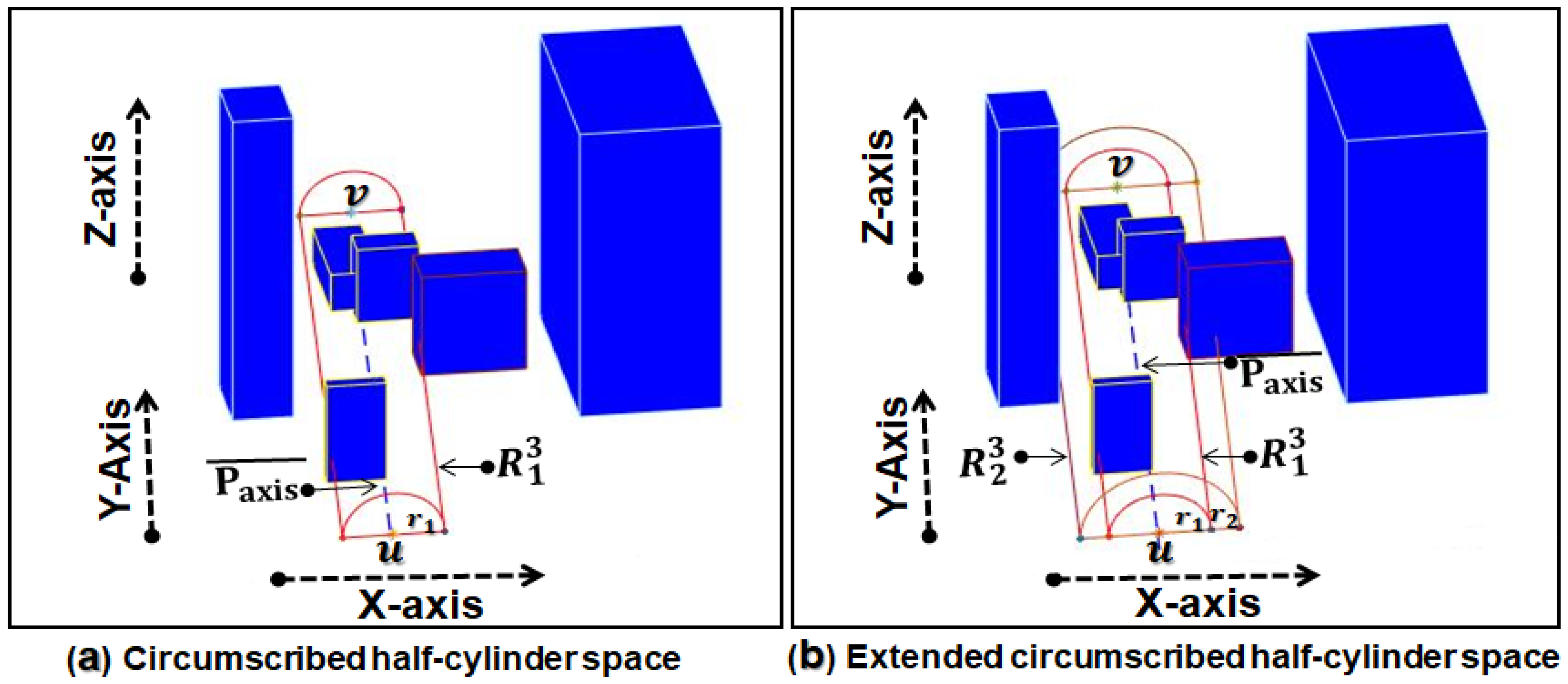
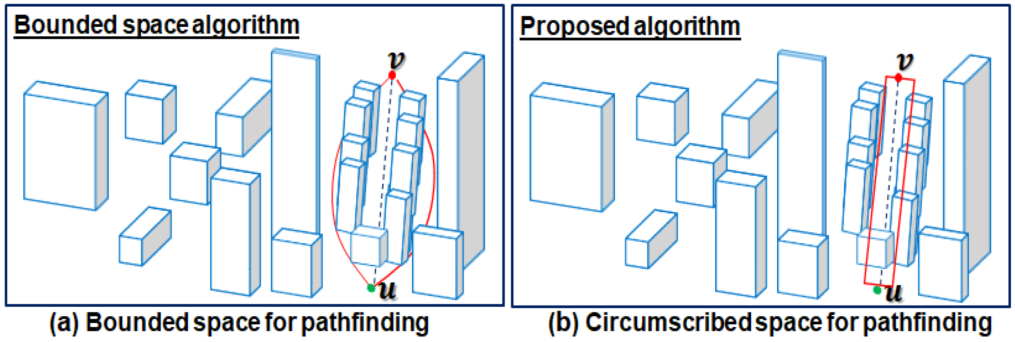
3.2. Formation of the Circumscribed Half Cylinder Space

Exploring a full map during path search can be very costly, and it may yield serious time performance issues in large and complex 3D environments. To effectively resolve this issue, we transform the 3D convex polyhedron fixed obstacles map into a circumscribed half cylinder space having source and target as endpoints with path guarantees to speed-up the pathfinding computations. The space circumscription process consists of five principle steps: (1) specifying source (u) and target (v) locations of UAV’s mission, (2) drawing primitive axis $\overline{P_{axis}}$ (a straight line) between u and v, (3) filtering relevant obstacles (e.g., those obstacles whose edges intersect with the $\overline{P_{axis}}$), (4) analysing the cross-section of filtered obstacles, (5) drawing minimum diameter $d_{min}$ half-circle such that the diameter of the half-circle is not fully covered by the sum of the cross-section of the obstacles that are on the $\overline{P_{axis}}$ between u and v. Upon reception of the u and v of the UAV mission, we draw a $\overline{P_{axis}}$ between u and v.

After drawing the $\overline{P_{axis}}$, three results can be obtained, such as: (1) no intersection and no collision, (2) no intersection but collision,(3) both intersection and collision. All three results are visually shown in Figure 3. If no obstacle intersects with the $\overline{P_{axis}}$, and collision can be avoided, then path $W=\overline{P_{axis}}$, which is a straight line path as shown in Figure 3a. Meanwhile, if no obstacle intersects with the $\overline{P_{axis}}$, but there exist some obstacles close to $\overline{P_{axis}}$ with whom UAV can possibly collide, then we take into account such obstacles and process them to generate a safe flight path between u and v as shown in Figure 3b. In the last scenario, as shown in Figure 3c, some obstacles intersect with the $\overline{P_{axis}}$ and we need to avoid them in an appropriate way to find the optimal or near-optimal collision-free path between u and v locations. These obstacles are filtered from a 3D map and are processed further. The complete pseudo-code used to filter relevant obstacles from the full map is given in Algorithm 1.

In Algorithm 1, map M containing N number of obstacles, source point u, and target point v are provided as an input. Set R, where (R⊆N) of relevant obstacles is obtained as an output. Line 2 implements the $\overline{P_{axis}}$ drawing between two locations u and v. Lines 3−7 perform the filtering of obstacles that intersect with the $\overline{P_{axis}}$. Finally, set R of relevant obstacles is returned (line 8). Meanwhile, if no obstacle lies between the source and target locations, then $R=\varnothing$ will be returned as an output.

Algorithm 1: Filtering relevant obstacles from the map.
	Input:	(1) Map M containing N number of obstacles, where $N=\{o_1,o_2,o_3,\cdots ,o_n\}$
		(2) Source point (u)
		(3) Target point (v)
	Output:	Set R of the relevant obstacles
	Procedure:
1	Initialize, set R = ∅
2	Draw primitive axis $\overline{P_{axis}}$ between (u) and (v)
3	for each $o_i$, where $o_i$ = $o_1$ to $o_n$ ∈ N do
4	if INTERSECTS ($\overline{P_{axis}}$, $o_i$) then
5	$R=R\cup \left\{o_i\right\}$
6	End if
7	End for
8	returnR

After obtaining set R of relevant obstacles, we apply the UAV flight height limits: minimum flight height limits ($h_{min}$), maximum flight height limits ($h_{max}$) and enlarge obstacles by safe distance ($D_{safe}$). After that, we analyze the cross-section of relevant obstacles that are on the $\overline{P_{axis}}$ between u and v. Then, we draw a minimum diameter half-circle keeping source location as the centre of the circle with path guarantees. We draw another half-circle of the same radius at the target side (i.e., keep target location as the centre of the half-circle) and join the bottom arcs of both half-circles with line segments. This results in a 3D C-space whose outlines can be regarded as a half-cylinder and we call this enclosed region a ‘circumscribed half cylinder space ’, denoted with $R_1^3$. This C-space transforms the more difficult geometric problem of finding a path for a UAV, considering its configuration and orientation around the real environment obstacles, into the easier dual problem of finding a path for a point around 3D convex obstacles. A pictorial overview of $R_1^3$ is given in Figure 4.

It encloses the relevant obstacles, either as a whole or only part of them. Additionally, due to the 3D environment, there can be some more obstacles which are not in set R but lying inside the $R_1^3$ partially or fully, we add those obstacles in set R and use them in the pathfinding process. The meaningfulness of $R_1^3$ is that it guarantees the collision-free path between u and v. Meanwhile, $R_1^3$ can or cannot be ideal for good quality (e.g., optimal or near-optimal) pathfinding due to several complex constraints related to obstacle geometry. By taking into account such constraints and optimal path probabilistic analysis (e.g., when several complex constraints exist in the $R_1^3$ related to obstacle geometry, a good quality path used to lie outside of the $R_1^3$ with very high probability), we perform multicriteria-based circumscribed half cylinder space complexity analysis.

3.3. Multicriteria-Based Circumscribed Half Cylinder Space Complexity Analysis

In order to determine whether $R_1^3$ is feasible for finding a path of good quality or not, a multicriteria-based complexity analysis of $R_1^3$ is performed. We find the complexity C of $R_1^3$ by exploiting detailed information about the obstacle geometry such as obstacle occupancy, obstacle placement, obstacles dominance and diversity of obstacle avoidance options that can hinders the path quality. There exists a strong correlation between path quality and space complexity criterions. The overall space complexity is the weighted sum of four criterions such as ratio of occupied spaces, diversity of obstacle avoidance options, dominance of the obstacles and ratio of overlapped obstacles. Brief details of the four criteria with equations and procedures are as follows.

3.3.1. Ratio of Occupied Spaces

To obtain a smooth and natural-looking path for UAV, it is desirable that obstacle occupancy in the space must be low. To quantify the obstacle occupancy in the circumscribed space, we find the total size (X) of the $R_1^3$, occupied spaces ($X_{obstacles}$) and free spaces ($X_{free}$). The total size (X) of the half-cylinder space can be obtained using Equation (1).

$$X=\frac{1}{2}\pi r^2\times l$$

(1)

where r is the radius of the half-circle and l is the Euclidian distance between u and v obtained using following equation.

$$l=\sqrt{{(x_t-x_s)}^2+{(y_t-y_s)}^2+{(z_t-z_s)}^2}$$

(2)

Out of the X sized space, we calculate amount of the space occupied by the obstacles ($X_{obstacles}$) using Equation (3).

$$X_{obstacles}=\sum _{i=1}^{N}V{O}_i$$

(3)

where N is the total number of the obstacles in $R_1^3$ and $V{O}_i$ is the volume of the obstacles. The volume of an obstacle $O_i$ can be calculated using following equation.

$$V{O}_i=O_h\times O_l\times O_w$$

(4)

where $O_h$, $O_l$, and $O_w$ represent the height, length and width of an obstacle respectively. The amount of the free space ($X_{free}$), where UAV can operate without collision with obstacles can be computed using Equation (5).

$$X_{free}=X\backslash X_{obstacles}$$

(5)

The ratio ($r_o$) of occupied space can be calculated using Equation (6).

$$r_o=\frac{X_{obstacles}}{X}$$

(6)

The value of $r_o$ ranges between 0 and 1. We use the ratio ($r_o$) of occupied space value in overall circumscribed space $R_1^3$ complexity calculations in Equation (15).

3.3.2. Diversity of Obstacle Avoidance Options

In both local and global path planning, there are generally four options, left, right, up and down (in case of flying or hanged obstacles), to avoid any obstacle a UAV finds during its course. Meanwhile, after the space circumscription, its highly likely that obstacle avoidance options will be reduced, and the diversity of the remaining options may increase. Because of this, a path may contain lots of turns and path length can increase. Therefore, while finding the space complexity, we consider the diversity of obstacle avoidance options. To calculate the diversity ($DOAO$) of each obstacle avoidance option category, the Simpson index [96] is used. It is known as the most simple and reliable measure for calculating $DOAO$. In our work, the path cannot be under an obstacle because the base height of all obstacles is zero, and therefore, a total of three options (e.g., top, left and right) are available to bypass any obstacle. The following procedure is used to calculate the $DOAO$ values from the circumscribed space.

• Calculate the proportion ($p_i$) of each obstacle avoidance option (e.g., $OA{O}_{left}$, $OA{O}_{right}$, $OA{O}_{top}$) category from the circumscribed space using Equation (7).

  $$p_i=\frac{OA{O}_i}{k}$$

  (7)

  where k is the total number of the obstacle avoidance options and it can be calculated using following equation.

  $$k=\sum _{j=1}^{3}OA{O}_j$$

  (8)
• Sum and square the individual proportions ($p_1,p_2,p_3,\cdots ,p_n$) of each obstacle avoidance option category from the circumscribed space. The result is diversity denoted with $DOAO$.

  $$DOAO=\sum _{i=1}^n{P}_i^2={\left(p_1\right)}^2+{\left(p_2\right)}^2+{\left(p_3\right)}^2+,\cdots ,+{\left(p_n\right)}^2$$

  (9)

Equation (9) gives the diversity of the obstacles avoidance options from the circumscribed space $R_1^3$. The value of $DOAO$ ranges between 0 and 1. The 0 value of $DOAO$ represents infinite diversity and 1, no diversity. To directly relate the value of $DOAO$ with the space complexity we do ($1-DOAO$) in our calculations. The greater the value of $DOAO$, the greater the obstacles avoidance options diversity, and vice versa.

3.3.3. Dominance of the Obstacles

Apart from the ratio of occupied spaces and diversity of obstacle avoidance options, another factor that introduces a serious performance bottleneck is the obstacle’s dominance. If most of the obstacles are centred at one place (i.e., the obstacle distribution is not uniform) in space, then the solution quality degrades. Obstacle dominance introduces cycles in a path because the path grazes many of the obstacles’ boundaries before reaching the target location. In order to calculate obstacle dominance, we divide $R_1^3$ into n small subspaces $\{S{S}_1,S{S}_2,S{S}_3,\cdots ,S{S}_n\}$ and find the dominance of each subspace. The obstacle dominance in a subspace ($S{S}_i$) is simply the ratio of the occupancy of the obstacles in the subspace divided by the total occupancy of all obstacles in the circumscribed space. For dominance calculations, the $R_1^3$ is divided into four subspaces ($n=4$). The dominance $D_i$ of the subspace $S{S}_i$ can be mathematically expressed as,

$$D_i=\frac{S{S}_{obstacles}^i}{X_{obstacles}}$$

(10)

where $X_{obstacles}$ is the total occupancy of all obstacles in the space as given in Equation (3) and $S{S}_{obstacles}^i$ is the occupancy of the obstacles in the subspace i, and it can be calculated using Equation (11).

$$S{S}_{obstacles}^i=\sum _{i=1}^{O^{{}^{\prime }}}V{O}_i^{{}^{\prime }}$$

(11)

where $V{O}_i^{{}^{\prime }}$ is the volume of the obstacles and $O^{{}^{\prime }}$ is the number of the obstacles in the subspace. After calculating the dominance of the n subspaces, we calculate the overall dominance $D_x$ of $R_1^3$ using Equation (12).

$$D_x=max\{D_1,D_2,D_3\cdots ,D_n\}$$

(12)

where $D_x$ is the dominance of the obstacles in the $R_1^3$. The main reason to take maximum values is to handle the worst cases effectively.

3.3.4. Ratio of Overlapped Obstacles

In some cases, there exist few obstacles which are not penetrated by the primitive axis, but they are overlapped with the relevant (e.g., the obstacles penetrated by the primitive axis) obstacles $O_i$. Such obstacles increase the path calculation time and, once calculated, it can contain many unnecessary turns, as stated by Frontera et al. [84]. Therefore, while evaluating the circumscribed space complexity, we take this factor into account along with the other three factors. The ratio of overlapped obstacles is simply the number of overlapped obstacles in the circumscribed space divided by the total number of relevant obstacles. The number of overlapped obstacles can be calculated using Equation (13).

$$N^{{}^{\prime }}=\sum _{i=1}^N(O_i\cup O_{EXT})$$

(13)

where $O_i$ denotes the relevant obstacles and $O_{EXT}$ represents the obstacles that intersects with the relevant obstacles $O_i$. The ratio of overlapped obstacles ($r_{oo}$) can be calculated using following equation.

$$r_{oo}=\frac{N^{{}^{\prime }}}{N}$$

(14)

where $N^{{}^{\prime }}$ denotes the number of overlapped obstacles and N represents the total number of relevant obstacles. When all four criterions values have been calculated, the overall complexity C of $R_1^3$ can be quantified using Equation (15).

$$C\left(R_1^3\right)=w_1\times r_o+w_2\times (1-DOAO)+w_3\times D_x+w_4\times r_{oo}$$

(15)

In Equation (15), $r_o$ denotes the ratio of occupied spaces, $DOAO$ means the diversity of the obstacle avoidance options, $D_x$ is the dominance of the obstacles in the space, and $r_{oo}$ is the ratio of the overlapped obstacles with the relevant obstacles. For the sake of simplicity, we used normalized values of each criterions, therefore the total complexity of the space has the range between 0 and 1. In the above equation, $w_i$, where $i=1,2,3,4$ denotes the weights of each criterion and they satisfy the two conditions, (i) $w_i>0$ and (ii) $w_1+w_2+w_3+w_4=1$. We adjust the weights by considering the contribution and importance of each criterion in the space complexity. The probability P of the optimal or near-optimal path W to be found from the first circumscribed space $R_1^3$ is given as

$$P\left(W\right)=\left\{\begin{array}{cc}1,\hfill & \mathrm{if}0<C\left(R_1^3\right)<T.\hfill \\ 0,\hfill & \mathrm{otherwise}.\hfill \end{array}\right.$$

(16)

where $C\left(R_1^3\right)$ is the complexity of $R_1^3$ and T is a threshold. The probability value 1 means that no space extension is needed because $R_1^3$ is good enough for finding an optimal or near-optimal path. Meanwhile, zero probability cases need space extension because $R_1^3$ fails to offer potential for good quality paths due to complex obstacle geometry. The threshold T value depends on the geometric factors present in the UAV operating environment, such as type of the mission, UAV manoeuvrability constraints and UAV resources. In our experiments, we used a threshold value of 0.65 to decide about the space extension. We performed rigorous experiments to verify the decision criteria using path length as the main objective. However, this value can be adjusted adaptively according to the UAV operating environment and available resources.

3.4. Extension of the Circumscribed Half Cylinder Space

Although the first circumscribed half cylinder space guarantees the path between source and target locations, it does not ensure the path quality in every scenario due to obstacle complexity. To effectively resolve this problem and ensure consistent quality, the scenarios which need space extensions are carefully identified though space complexity analysis. Through the use of multicriteria-based complexity analysis of $R_1^3$, we were able to accurately identify the scenarios which need relatively bigger space than $R_1^3$. Having complete information about the obstacles intersected by the surface of $R_1^3$ enabled us to extend the space to the next level with ease. We choose this procedure to extend the space since it yields much less computing overhead in space extension and significantly improves path quality . Therefore, by including the obstacles that were crossed by the surface of the $R_1^3$ and drawing a half-circle in a similar way as we did for the first space creation result into a second circumscribed half cylinder space of relatively bigger size than $R_1^3$ as shown in Figure 5b.

We call this space an extended space, denoted with $R_2^3$ inclusive of $R_1^3$. The extended space fully includes relevant obstacles and it offers potential for a path to be obtained solely from the extended space $R_2^3$. As mentioned earlier, due to the 3D environment, more obstacles can become part of $R_2^3$, so we add those obstacles in set R and use them in the pathfinding process. The meaningfulness of $R_2^3$ is that it is the space from which good quality paths (i.e., the obtained path length is close to the optimal or near-optimal paths) can be obtained with very high probability. The space can be extended further in an analogous way up to the $n^{th}$-level. Meanwhile, in our algorithm, we extend the spaces up to two levels only because optimal path tends to lie in $R_1^3$ and $R_2^3$ with a very high probability. Once the decision about the appropriate space has been made, a visibility graph is generated from the selected circumscribed space for pathfinding.

3.5. Sparse Visibility Graph Generation

Visibility graph (VG) is one of the most widely used approaches for UAV pathfinding in a known environment. VG constructs a compact, undirected graph connecting u with v by capturing the connectivity of $X_{free}$ to form a network of paths. Due to its simplicity and effectiveness in shortest pathfinding, VG has been widely used in many applications. However, constructing a VG is computationally expensive and the time complexity of constructing VG is $O\left(n^3\right)$, where n is the number of vertices. Much work on reducing the complexity of VG construction has been carried out by changing obstacle shapes, merging nearby obstacles and ignoring tiny obstacles. More recent evidence [84] shows that time complexity of VG can be reduced to $O\left(n^2\right)$ in 3D environments by only taking into account the straight line path obstacles.

To further reduce the visibility graph construction time complexity, this paper proposes a sparse visibility graph (SVG) construction algorithm which does not construct the complete visibility graph. This algorithm constructs an SVG from the circumscribed space in the form of a roadmap which has connectivity between u and v via intermediate nodes. Mathematically, SVG is a double edge graph G of inter-visible locations: $G=\{V,E\}$. There are two steps to constructs G from a 3D C-space: sampling the nodes set V and creating the edge set E. The first step involves the generation of nodes set V. We used the top, bottom and mid vertices of the obstacles to make the SVG. The top and bottom vertices of the obstacles are known in the form of 3D points (i.e., $x,y,z$) and mid vertices can be computed on the adjacent edges by employing the midpoint formula. Each obstacle has total eight vertices. The vertices of the $ith$ obstacle along with the values can be mathematically expressed in following matrix

$$O_i=\left[\begin{array}{ccccc}{x}_{min}& y_{min}& z_{min};x_{min}& y_{min}& z_{max}\\ x_{min}& y_{max}& z_{min};x_{min}& y_{max}& z_{max}\\ x_{max}& y_{min}& z_{min};x_{max}& y_{min}& z_{max}\\ x_{max}& y_{max}& z_{min};x_{max}& y_{max}& z_{max}\end{array}\right]=\left[\begin{array}{ccccc}100& 200& 0;100& 200& 190\\ 100& 240& 0;100& 240& 190\\ 190& 200& 0;190& 200& 190\\ 190& 240& 0;190& 240& 190\end{array}\right]$$

(17)

The bottom four vertices are generalized to the $h_{min}$ of the UAV and top vertices of the obstacles have height values equal to half-circle radius. For example, for an obstacle whose actual height is higher than the half-circle radius while the top and bottom vertices are given, the set of mid vertices pairs on both the vertical faces $F_1$ and $F_2$ can be computed using Equations (18) and (19).

$$F_1=\{x_{min},y_{min},\frac{z_{max}+z_{min}}{2}\},\{x_{min},y_{max},\frac{z_{max}+z_{min}}{2}\}$$

(18)

$$F_2=\{x_{max},y_{min},\frac{z_{max}+z_{min}}{2}\},\{x_{max},y_{max},\frac{z_{max}+z_{min}}{2}\}$$

(19)

After finding the nodes set V from the relevant obstacles edges, we add the pair of u and v in set V and create the edge set E via visibility checks. Two nodes p and q in nodes set V are mutually visible if the line segment $\overline{pq}$ joining them does not intersect with any obstacle. The line of sight (LOS) checking function determines the visible connection between the pair of nodes located on the same obstacle as well as on different obstacles. More details on adding the collision free edges between visible vertices by exploiting the convex characteristics of the obstacles are given in our previous paper [85]. The time complexity of the edges creation process heavily depends on the LOS checking function. Meanwhile, in our work, we reduce the time complexity of the LOS checking function by taking direction into account; that is, it only adds the edges between a pairs of vertices that lead to the direction of the target. We set the visibility of the pair of vertices to false using co-ordinate values that are on the same obstacle but lead to the opposite direction of the target. Therefore, with the linear time complexity of the visibility checking function, the time complexity of SVG creation is $O\left({\left(nkf\right)}^2\right)$ time where n is number of obstacles, k is the number of levels, and f is the number of facets. Meanwhile, k has a constant upper bound therefore, the time complexity of SVG is $O\left({\left(nf\right)}^2\right)$. Due to less number of obstacles and facets our algorithm is a clear improvement over related studies. With the help of the node set V and edge set E, a graph G is obtained from the circumscribed space which connects u and v, and it possess all properties of a roadmap.

3.6. Path Searching

After an SVG is constructed, the pathfinding algorithm is applied to search for the path W. In our work, we used $A^{*}$ algorithm for collision-free pathfinding between u and v on SVG. A* is considered as one of the best heuristic-based optimization algorithms for finding the paths of low cost. A* search avoids expanding the paths that are expensive in terms of path lengths. The evaluation function (i.e., an estimation of path length) used by A* algorithm is given in Equation (20).

$$f\left(n\right)=g\left(n\right)+h\left(n\right)$$

(20)

where $f\left(n\right)$ represents the estimated total cost of path between source and target location through the node n, $g\left(n\right)$ represents the exact path length to reach to node n, and $h\left(n\right)$ is the heuristic function which estimates the cost from node n to target location. $A^{*}$ algorithm was chosen to speed up the path searching process over SVG. After the exploration of the SVG using $A^{*}$ algorithm, the path W is obtained. In our work, we calculate the path length and computation time for quantifying the quality of the obtained paths. However, in some cases, the obtained path W cannot be the true shortest path, which requires a post-processing step to optimize it.

3.7. Path Length Optimization

In most UAV applications, the length of the planned path is extremely important, and it should be held to a minimum to preserve UAV resources. However, degradation in path length is an unfortunate and inevitable consequence of any path planning algorithm with reduced search space. To circumvent this issue, we optimize the length of the obtained path W by adding more nodes around the initial path nodes. Our proposed path optimization method is mainly carried out in three steps. To begin with, it tries to determine the adjacent neighbour nodes of the path W nodes. Later, we find the distance between the path nodes and their adjacent neighbour nodes. On the closest half region around the initial path nodes, we add more nodes with dense resolution ($D_{res}$) and on the farthest half region with sparse resolution ($S_{res}$). The reason to cluster more nodes around the initial path nodes is that all nodes possess visibility, and path length can be significantly optimized. After adding more nodes, a path of optimized length is obtained using the newly discovered and initial path nodes by applying the same mechanism as explained in former subsections. This path-refining method reduces the path length significantly with much less computing overhead.

4. Results and Discussion

This section demonstrates the output of the discussed concepts . The improvements of the proposed algorithm were compared using two criteria; the improvements in computation time and path lengths with the existing closely related algorithms. To benchmark the proposed algorithm, we compared the proposed algorithm results with visibility graph-based and randomized motion planning approaches. All the simulation results were produced and compared on a PC running Windows 10, with a CPU of 2.6 GHz and 8.00 GB of RAM, using MATLAB version 9.4.0.813654 (R2018a). In the proposed algorithm simulations, we consider a 25-kg fixed wing UAV similar to our previous work [85]. We considered both local and global constraints during the simulations. The numerical values related to local constraints (i.e., UAV itself) are: maximum steering angle: $\pi /6$ radius and wing span: 1 m. The minimum and maximum UAV flight height limits are 22 m and 150 m ($h_{min}=22$ m, $h_{max}=150$ m). The global constraints are related to the obstacle’s composition in the environment. We consider four dominant constraints such as obstacle occupancy, obstacle dominance, diversity of obstacle avoidance options and overlapped obstacles in space size selection that can impact solution quality as well as UAV safety. We assumed that the UAV has sufficient battery to finish the mission successfully. The safe distance is set to 10 m ($D_{safe}=10$ m) for collision avoidance with obstacles. We assumed a zero-wind scenario during the flight. The proposed approach finds paths using visibility graph that respect both local and global constraints. The initialization of the parameters of our algorithm: the weights of each space complexity criterions are 0.2, 0.2, 0.3 and 0.3 ($w_1=0.2$, $w_2=0.2$, $w_3=0.3$, $w_4=0.3$). The dense and sparse resolutions are 10 m and 15 m ($D_{res}=10$ m, $S_{res}=15$ m) for path length optimization.

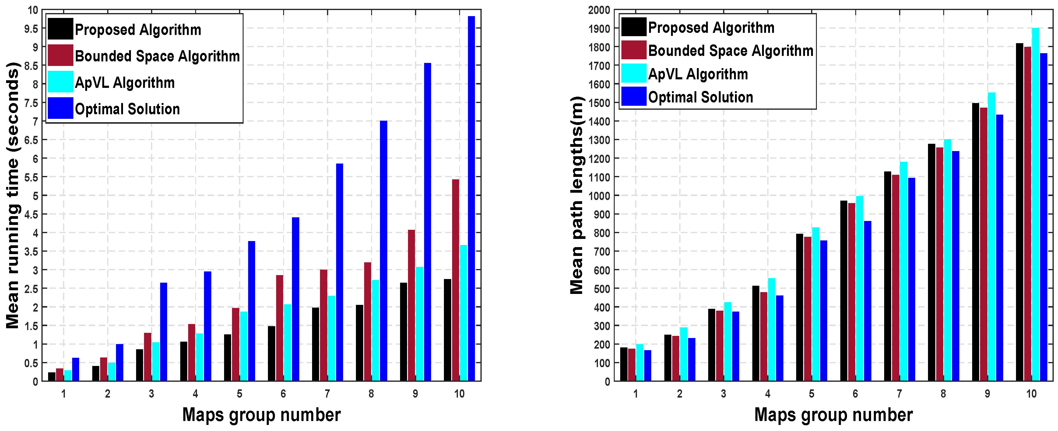
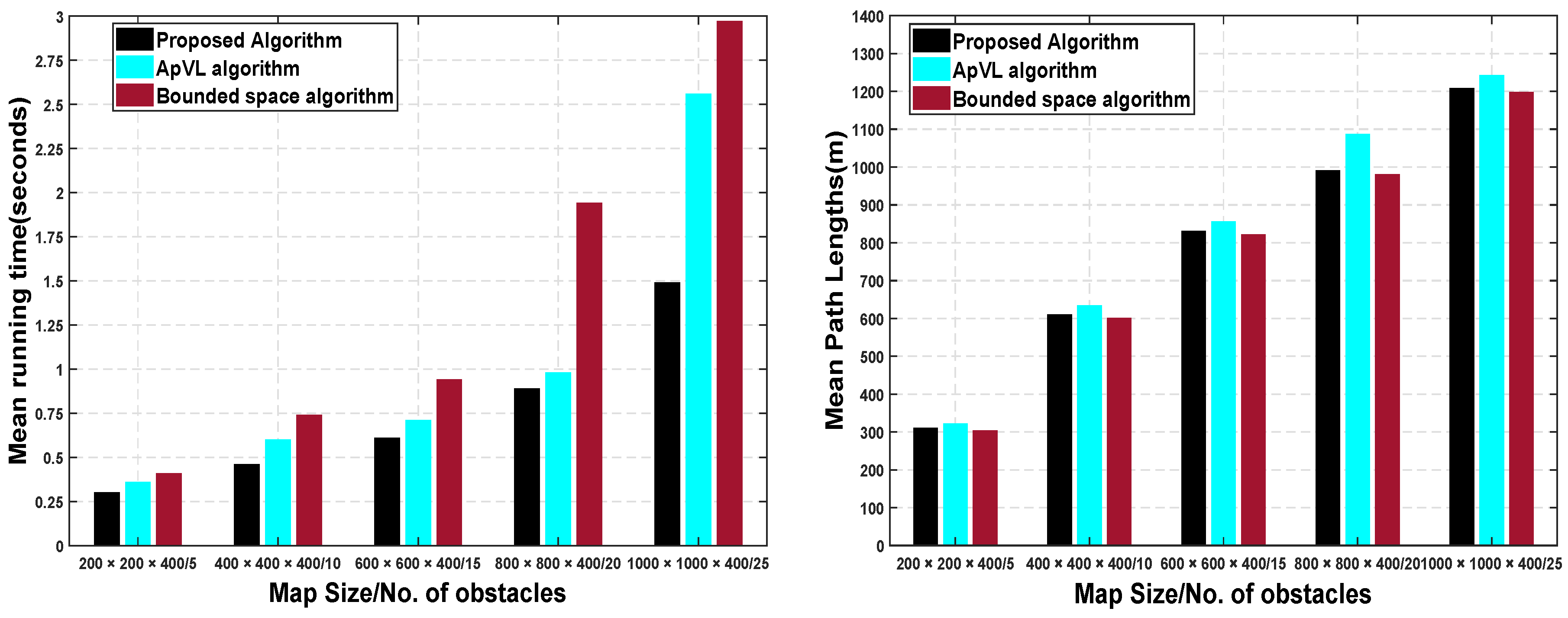
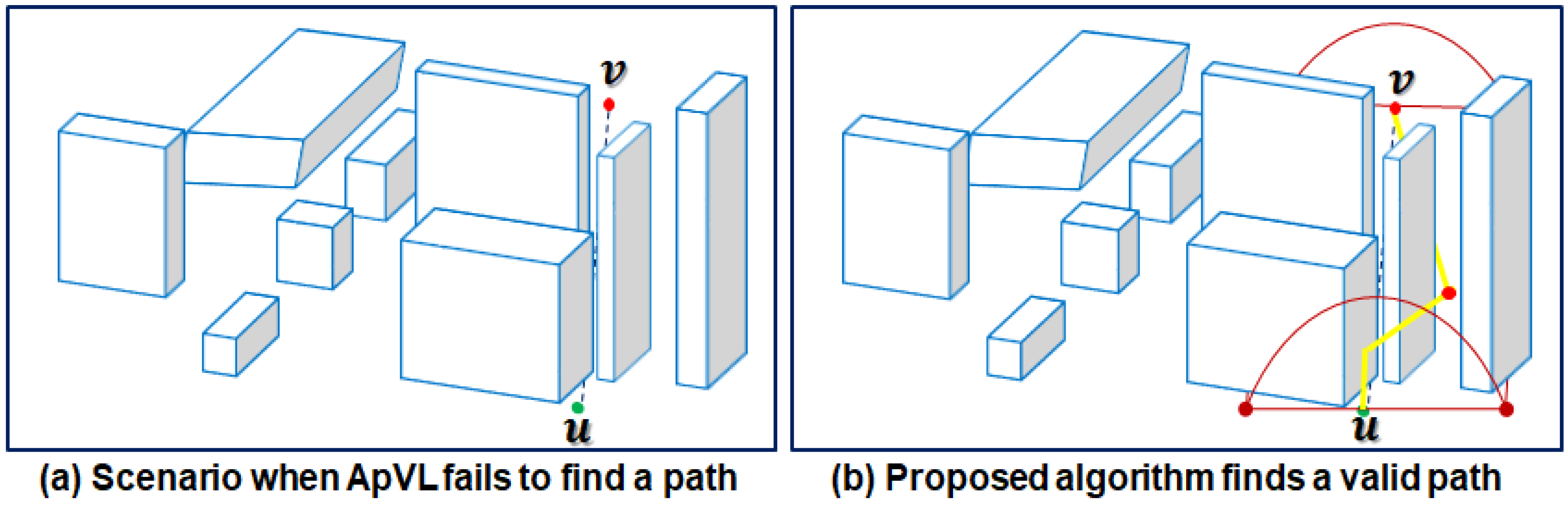
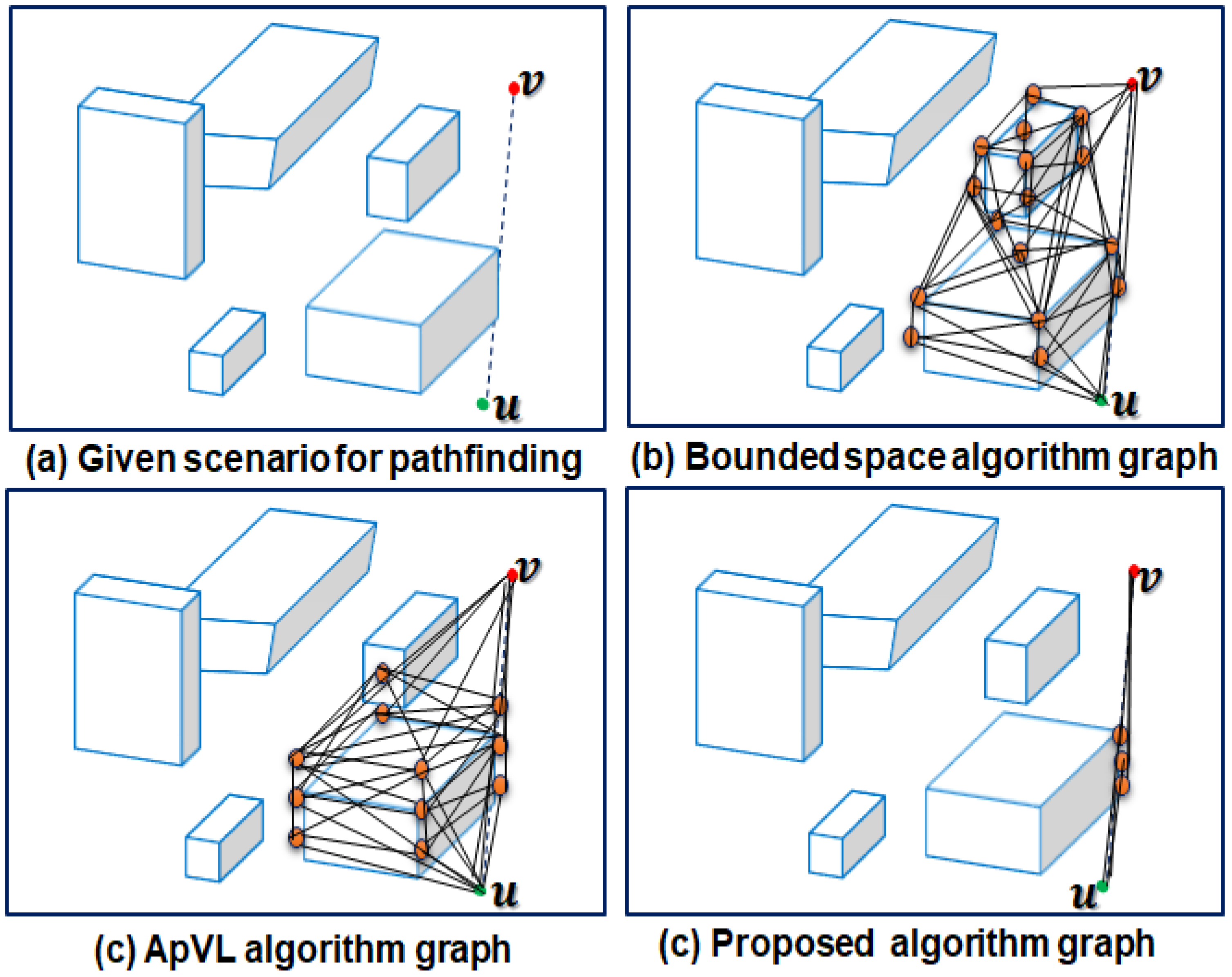
4.1. Comparison with the Visibility Graph-Based Approaches

We compared the proposed algorithm performance with two visibility graph-based path planning algorithms which are closely related to the proposed study in many aspects. To assess the performance of the proposed algorithm, we designed three different scenarios of 3D environments with obstacles. Every scenario is solved using three algorithms, including our own, and the results are then compared. Obstacles have a rectangular base with random width, depth, and height. The details about map sizes, number of maps, source and target locations, obstacle counts and obstacle dimensions, etc. are explained in each scenario. We present the overview of the 3D maps used in the experiments and two exemplary results visually with length values of all three algorithms (ApVL algorithm [84], Bounded space algorithm [85] and the proposed algorithm) paths in Figure 6.

Scenario (I) is defined within an operational area of size $100\times 100\times 300-1000\times 1000\times 400$. It includes one hundred maps with random numbers of obstacles (between five and 50). For the convenience of comparing algorithm performance, we arranged all one hundred maps in ten groups based on map size and obstacle counts as shown in

Table 1. Description about the maps used in experiments and operating environment modelling results.

Group No.	Map Size/No. of Obstacles	Proposed Algorithm	ApVL Algorithm	Bounded Space Algorithm
	(x × y × z)/(5 − 50)	Avg. Running Time (s)	Avg. Running Time (s)	Avg. Running Time (s)
1	100 × 100 × 300/5	0.91	1.16	2.67
2	200 × 200 × 300/10	4.91	7.39	12.89
3	300 × 300 × 300/15	15.06	20.57	28.21
4	400 × 400 × 300/20	36.13	46.56	57.24
5	500 × 500 × 300/25	72.56	93.84	110.64
6	600 × 600 × 400/30	96.67	106.17	136.81
7	700 × 700 × 400/35	129.63	132.59	176.93
8	800 × 800 × 400/40	151.51	181.49	207.19
9	900 × 900 × 400/45	176.31	195.26	221.33
10	1000 × 1000 × 400/50	187.22	204.30	242.49

. The start point u and target point v of the UAV mission are located on different places in each map. To benchmark the proposed path planning algorithm with other existing methods, the proposed method results are compared with ApVL [84] and bounded space [85] algorithms, both of which have been demonstrated as being better than other methods in terms of computing speed and path lengths when finding paths in 3D environments. Besides the two existing algorithms, we compare the algorithm performance with the optimal solution that is obtained from utilizing the full map information and very dense VG with fine resolution. Depending upon the u and v locations and obstacle placement in each map, the algorithms will tackle a different number of obstacles to find a path W. The area covered by the obstacles is different from map to map.

The ApVL algorithm [84] only processes straight line path obstacles and uses dense VG to find paths incrementally. Meanwhile, the ApVL method incurs a high time cost and yields non-taut paths in many situations. Bounded space algorithm [85] performs path searches on relatively large space (i.e., process a larger number of obstacles) and use dense VG. The paths produced by this algorithm are shorter in length, but computation time is very high. On the other hand, the proposed algorithm processes fewer number of obstacles and uses SVG to find paths of good quality. It also introduces a viable solution to effectively resolve the optimality and speed trade-off by optimizing the path length at the end with much less computing overhead. The environment for each run is different due to the random positions of the obstacles. The complete description regarding the maps used in this scenario and average running time of environment modelling of the proposed algorithm and its comparisons with the two existing algorithms is shown in Table 1.

The environment modelling time shown in Table 1 is the sum of the circumscribed space formation, SVG construction, and SVG enhancement time for path length optimization. Through simulations and comparison with the two existing algorithms, on average, our algorithm reduces the computing time of UAV operating environment modelling by 18.65%. The pathfinding performance results in terms of the running time and their comparison with the two state-of-the-art methods and optimal solution is shown in Figure 7 (Left). The computational time is the average of ten maps in each group (listed in Table 1) with random obstacle placement. The mean path length results and their comparison with the two state-of-the-art methods and optimal solution are shown in Figure 7 (Right). These results show that, for each algorithm, the computation time increases with the increase in map size and number of obstacles. Meanwhile, the proposed algorithm shows 11.9% and 26.3% reduction in mean computational time as compared to ApVL and bounded space method, respectively.

From the comparisons with the optimal solution, our proposed algorithm lowers the computation time of pathfinding by 39.41%. The proposed algorithm reduces the computational time of pathfinding significantly by searching for paths on high priority spaces using SVG. From path lengths point of view, the proposed algorithm shows 8.33% improvements in mean path length compared to the ApVL algorithm. Meanwhile, average degradation in path lengths for our proposed algorithm with respect to bounded space and optimal solution are only 3.41%. The marginal degradation in path lengths is possibly due to complex obstacle arrangement that can be optimized by extending space or decreasing graph resolution values.

Scenario (II) contains ten maps with a pre-determined number of obstacles over an operational area of 1 km² to assess impacts of increased obstacles on algorithm performance. These obstacles are placed in 3D environments in such a way that all obstacles will be processed to obtain the final path.

Table 2. Proposed algorithm pathfinding performance with varying number of obstacles.

No. of Obstacles	Proposed Algorithm		ApVL Algorithm		Bounded Space Algorithm
	Avg. Time (s)	Length Ratio	Avg. Time (s)	Length Ratio	Avg. Time (s)	Avg. Length (m)
10	0.15	1.02298	0.28	1.05371	0.63	482.33
20	0.63	1.01350	0.87	1.01983	1.97	1093.94
30	1.02	1.01722	1.30	1.02577	2.04	1169.02
40	1.10	1.05135	1.37	1.08586	3.05	1283.12
50	1.30	1.01384	2.76	1.03214	3.25	1639.66
60	1.38	1.01071	2.92	1.01606	4.57	1681.23
70	1.53	1.00511	3.03	1.01589	5.03	1868.77
80	1.87	1.00527	3.32	1.01577	5.24	1904.50
90	2.32	1.00659	4.06	1.01492	6.08	2004.32
100	2.98	1.00768	4.29	1.01393	7.30	2210.53

summarizes the results of our proposed algorithm with varying numbers of obstacles and its comparison with the two existing algorithms. The bounded space algorithm [85] provides the shortest path whose length is very close to the optimal solution (although it finds paths at a very high time cost). Therefore, we used the path provided by the bounded space algorithm [85] as a reference path to measure the quality of paths produced by the proposed and ApVL algorithms. We reported the average path lengths of the bounded space algorithm, and path lengths in the form of ratios for our proposed algorithm and ApVL algorithm in Table 2. When the environment becomes crowded with obstacles, our algorithm can find a collision-free and good quality path inside these areas efficiently. The proposed method is superior than the ApVL and bounded space methods in computation time even with an increased number of obstacles. The paths produced by the proposed algorithm are shorter and smoother than the ApVL algorithm and only marginally longer than the bounded space method. Through simulations and comparison with the two existing algorithms on these ten obstacle counts specific maps, on average, our proposed algorithm reduces the computing time of pathfinding by $31.08\%$. From a path length point of view, the paths produced by our algorithm are only marginally (0.01–1.3%) longer than the reference paths.

Scenario (III) is defined within an operational area of size $200\times 200\times 400-1000\times 1000\times 400$. It includes five maps with random numbers of obstacles (between five and 25). We compared the algorithms through five experiments on each map with alternate locations of the u and v in each run to validate the applicability and efficiency of the proposed algorithm for practical purposes. By changing the locations of u and v, the number of obstacles processed in each run can be different and, accordingly, the path length and computation time may wary. The proposed algorithm averages obtained from 25 runs are shown in Figure 8.

The proposed algorithm gives the average running time value of 0.75 s as compared to ApVL and bounded space algorithms that give mean running time values of 1.04 s and 1.54 s, respectively.

From a path length point of view, the proposed algorithm improves path length by $5.3\%$ compared to the ApVL algorithm and shows marginal degradation ($1.28\%$) compared to the bounded space algorithm. These results emphasize the validity of the proposed algorithm with respect to achieving better computational time and improved path lengths. Apart from the numerical result companions, we compared the proposed algorithm results in three unique aspects with the existing visibility graph-based algorithms.

A. Compared with the previous solution in search space size:Figure 9 shows the search space selected by the bounded space and proposed algorithm for pathfinding. From the results, it can be seen that bounded space algorithm Figure 9a unnecessarily considers more space compared to the proposed algorithm Figure 9b. The collision-free path lies along the straight-line and it can be computed by avoiding only one obstacle. Ignoring the obstacles complexity in space reduction process dramatically increases the solution cost. In contrast, the proposed algorithm considers the obstacles’ complexity and circumscribes the search space of small size which is enough for good quality collision-free pathfinding. In the given scenario, the proposed algorithm only considers one relevant obstacle. Meanwhile, bounded space algorithm processes nine obstacles causing a very high time performance overheads.

B. Compared with the previous solution in path guarantees (i.e., completeness): ApVL algorithm [84] does not guarantee the path from the selective part of the UAV’s C-space due the presence of the nearby obstacles. Figure 10 presents a scenario where the ApVL algorithm [84] fails to find a path even though it exists. Ignoring the path guarantees in the space reduction process, instead of considering only the straight-line path obstacles which is not an effective method of reducing computing time of pathfinding in a fine-grained manner. However, the proposed algorithm always guarantees a path from the selective part of the UAV’s C-space.

C. Compared with the previous solutions in graph size: Most of the visibility graph-based path planning algorithms are prone to very high time performance overheads due to the extensive visibility checks. In order to effectively resolves this issue, we generate sparse graph considering the goal direction with only few nodes and edges. Figure 11 shows the graph size for finding a path from a 3D environment involving five obstacles. From the results, it can be observed that the proposed algorithm contains only fewer potential nodes. The proposed algorithm performs less number of visibility checks compared to ApVL [84] and bounded space [85] during SVG construction which significantly reduces the computation load.

Although the proposed approach is a major advance, a high number of initial path nodes can limit its performance. The worst case time complexity of the proposed algorithm is $O\left(n^3\right)$. However, simulation results show that computing time does not increase as fast as $O\left(n^3\right)$ in all three scenarios while finding paths of comparable lengths. The results obtained from all three scenarios and three examples emphasize the validity of the proposed algorithm with respect to achieving better computing time, improved path length, and lower computational complexity. This study provides additional support for quick pathfinding compared to the current state-of-the-art and closely related methods. The findings appear to be well substantiated for both accuracy and efficiency.

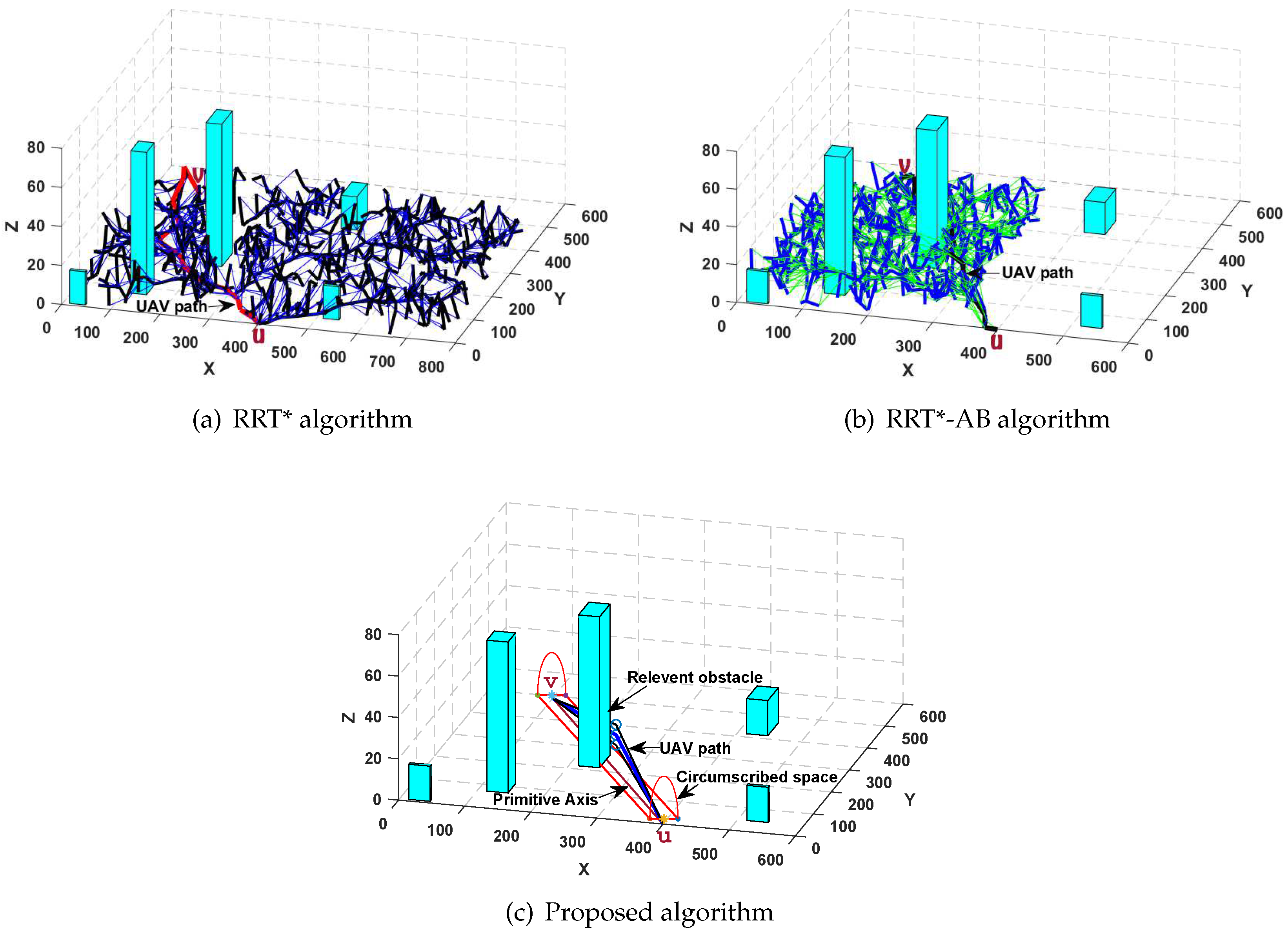
4.2. Comparison with the Randomized Motion Planning Techniques

To further validate the proposed algorithm’s feasibility and effectiveness, we compared the proposed algorithm results with the RRT* algorithm [92] and its improved version RRT*-AB [95]. RRT* algorithm [92] is superior compared to RRT due to the two optimization procedures in the extend function. It ignores the connection of high cost and retains only the low cost vertices to obtain a path with minimum cost. RRT*-AB [95] shows clear improvements in path lengths and convergence rate as compared to the earlier versions of RRT* algorithm. The proposed approach bounds the search space between the initial and goal locations. It performs intelligent sampling in the bounded space for tree construction. Once an initial path is found, the proposed approach optimizes the path length using three strategies such as concentrated sampling, node rejection and path pruning. The RRT*-AB approach has slow convergence rate, and it performs extensive rewiring in finding the optimal path. In contrast, the proposed algorithm chooses the appropriate space intelligently for low cost pathfinding with fewer nodes. Figure 12 shows a pictorial overview of the proposed algorithm, RRT*-algorithm and RRT*-AB algorithm path results obtained from a 3D environment.

In Figure 12, our proposed algorithm gives path length value of 594.54 m, as compared to RRT* and RRT*-AB algorithms that give path length values of 627 m and 614 m respectively. In terms of computational efficiency, the proposed algorithm is faster and features lower computational complexity across experiments. To compare the proposed algorithm results, we select five maps from each map groups listed in Table 1 and perform five experiments on each map with random numbers of obstacles (between 5 to 50). The average computation times and path lengths obtained from the simulations are summarized in

Table 3. Proposed algorithm pathfinding performance comparison with RRT* and RRT*-AB algorithms.

Maps Group No.	RRT* Algorithm		RRT*-AB Algorithm		Proposed Algorithm
	Avg. Time (s)	Avg. Length (m)	Avg. Time (s)	Avg. Length (m)	Avg. Time (s)	Avg. Length (m)
1	10.23	245.13	7.21	175.67	1.14	178.24
2	22.40	275.34	14.44	244.19	5.31	248.27
3	31.94	423.12	28.06	389.23	15.91	381.77
4	61.53	546.43	46.66	524.32	37.18	504.69
5	99.49	839.22	89.19	828.45	73.82	791.34
6	182.62	1039.56	161.61	997.67	98.14	969.17
7	234.47	1240.96	202.18	1159.86	131.60	1126.34
8	286.58	1465.25	213.55	1308.12	153.55	1276.29
9	321.81	1542.65	267.12	1509.87	178.95	1491.89
10	415.45	1992.58	287.21	1896.18	189.97	1826.24

. The average time shown in Table 3 is the sum of the modelling phase (i.e., graph/tree construction) and path searching phase.

The results clearly illustrate that the proposed algorithm yields more time efficient and near-optimal paths, with the exception of the first two cases, where the RRT*-AB has improved path lengths due to the small scale 3D environments with only fewer obstacles. It is clear that, as the environment size and number of obstacles grow, the performance of the proposed approach improves on both metrics (i.e., running time and path lengths). Through simulations and comparison with the RRT* and RRT*-AB, on average, our algorithm reduces the overall time required to compute an optimal/near-optimal path by 38.45%. From the path lengths point of view, it lowers the path lengths by 5.6% in most cases. Besides the computing times and path lengths, we compared the proposed algorithm performance with RRT* and its variant on the basis of number of path nodes and tree/graph nodes. In

Table 4. Average graph/tree nodes and path nodes: proposed algorithm versus RRT* and RRT*-AB.

Algorithms	Evaluation Criteria	Maps Group No.
		1	2	3	4	5	6	7	8	9	10
RRT*	Avg. tree nodes Avg. path nodes	300 17	500 21	650 28	825 31	1045 39	1235 35	1479 41	1979 37	2129 43	2521 44
RRT*-AB	Avg. tree nodes Avg. path nodes	221 13	351 16	423 14	549 19	661 21	835 24	1056 29	1461 29	1598 34	1932 40
Proposed	Avg. graph nodes Avg. path nodes	112 5	198 8	276 9	342 13	467 15	681 17	799 21	981 24	1292 27	1538 31

, the performance of the proposed approach in terms of average graph/tree nodes and path nodes for the aforementioned experiments is presented. As given in the last two rows of Table 4, the graph nodes and number of path nodes of the proposed SVG approach are much lower than other methods.

The proposed algorithm is complete, and it is applicable for various UAV missions. The proposed algorithm performs well regarding good quality pathfinding for two reasons: (1) the novel space circumscription method is introduced, which not only reduces computation time by constraining the path search to the high priority space, but also helps in finding an optimal or near-optimal path with very high probability; and (2) the SVG, which generates a very sparse visibility graph, reduces the computation time of pathfinding significantly by allowing direction oriented target search. The proposed algorithm resolves time performance issues stemming from the size of the search space and needless path searches on low priority spaces, and in addition, it overcomes the difficulty of pathfinding for UAVs in an obstacle-rich environment.

5. Conclusions and Future Work

In this paper, we proposed a global flight path planning algorithm based on space circumscription and sparse visibility graph for unmanned aerial vehicles (UAVs) in three-dimensional (3D) environments with fixed convex obstacles. The main goals of the proposed algorithm are to reduce the computing time of both environment modelling and pathfinding without significantly impacting the path quality for UAVs flying at low-altitudes in 3D environments. We devised a novel method by exploiting the information about obstacle geometry to circumscribe the search space in the form of a half cylinder that guarantees an optimal or near-optimal path with significantly reduced time cost. We generate a sparse visibility graph from the circumscribed space and find the initial path, which is subsequently optimized by adding more nodes around the initial path nodes. The proposed algorithm effectively resolves the efficiency and optimality trade-off, and in most cases, it consistently performs better than state-of-the-art and closely related global flight path planning algorithms. It reduces pathfinding computing time significantly by constraining path searches only to the high priority circumscribed space and, at the same time, find paths that are only marginally longer than the optimal path. In future work, we are planning to enhance the proposed algorithm by incorporating in-depth obstacle geometry information for more intelligent space circumscription and visibility graph generation. Furthermore, we are focusing to apply the proposed approach in space decomposition for UAV coverage tasks in urban settings due to its simplicity, effectiveness, ease of implementation and less computational complexity. Finally, we intend to extend the proposed algorithm for solving multi-objectives path planning problems in large and complex 3D environments.

References

1. Song, B.D.; Park, K.; Kim, J. Persistent UAV delivery logistics: MILP formulation and efficient heuristic. Comput. Ind. Eng. 2018, 120, 418–428. [Google Scholar] [CrossRef]
2. Haidari, L.A.; Brown, S.T.; Ferguson, M.; Bancroft, E.; Spiker, M.; Wilcox, A.; Ambikapathi, R.; Sampath, V.; Connor, D.L.; Lee, B.Y. The economic and operational value of using drones to transport vaccines. Vaccine 2016, 34, 4062–4067. [Google Scholar] [CrossRef] [PubMed] [Green Version]
3. Torresan, C.; Berton, A.; Carotenuto, F.; di Gennaro, S.F.; Gioli, B.; Matese, A.; Miglietta, F.; Vagnoli, C.; Zalde, A.; Wallace, L. Forestry applications of UAVs in Europe: A review. Int. J. Remote Sens. 2017, 38, 2427–2447. [Google Scholar] [CrossRef]
4. Sarris, Z.; Atlas, S. Survey of UAV applications in civil markets. In Proceedings of the IEEE Mediterranean Conference on Control and Automation, Corfu, Greece, 20–23 June 2011; p. 11. [Google Scholar]
5. Näsi, R.; Honkavaara, E.; Blomqvist, M.; Lyytikäinen-Saarenmaa, P.; Hakala, T.; Viljanen, N.; Kantola, T.; Holopainen, M. Remote sensing of bark beetle damage in urban forests at individual tree level using a novel hyperspectral camera from UAV and aircraft. Urban For. Urban Green. 2018, 30, 72–83. [Google Scholar] [CrossRef]
6. Yuan, C.; Zhang, Y.; Liu, Z. A survey on technologies for automatic forest fire monitoring, detection, and fighting using unmanned aerial vehicles and remote sensing techniques. Can. J. For. Res. 2015, 45, 783–792. [Google Scholar] [CrossRef]
7. Kanistras, K.; Martins, G.; Rutherford, M.J.; Valavanis, K.P. A survey of unmanned aerial vehicles (UAVs) for traffic monitoring. In Proceedings of the 2013 International Conference on Unmanned Aircraft Systems (ICUAS), Atlanta, GA, USA, 28–31 May 2013. [Google Scholar]
8. Stöcker, Cl.; Eltner, A.; Karrasch, P. Measuring gullies by synergetic application of UAV and close range photogrammetry—A case study from Andalusia, Spain. Catena 2015, 132, 1–11. [Google Scholar] [CrossRef]
9. Erdelj, M.; Natalizio, E.; Chowdhury, K.R.; Akyildiz, I.F. Help from the sky: Leveraging UAVs for disaster management. IEEE Pervasive Comput. 2017, 16, 24–32. [Google Scholar] [CrossRef]
10. Liao, K.-W.; Lee, Y.-T. Detection of rust defects on steel bridge coatings via digital image recognition. Autom. Constr. 2016, 71, 294–306. [Google Scholar] [CrossRef]
11. Sujit, P.B.; Sousa, J.; Pereira, F.L. UAV and AUVs coordination for ocean exploration. In Proceedings of the Oceans 2009-Europe, Bremen, Germany, 11–14 May 2009. [Google Scholar]
12. Zikidis, K.C. Early Warning Against Stealth Aircraft, Missiles and Unmanned Aerial Vehicles; Surveillance in Action; Springer: Cham, Switzerland, 2018; pp. 195–216. [Google Scholar]
13. Raja, P.; Pugazhenthi, S. Optimal path planning of mobile robots: A review. Int. J. Phys. Sci. 2012, 7, 1314–1320. [Google Scholar] [CrossRef]
14. Nikolos, I.K.; Valavanis, K.P.; Tsourveloudis, N.C.; Kostaras, A.N. Evolutionary algorithm based offline/online path planner for UAV navigation. IEEE Trans. Syst. Man Cybern. Part B (Cybern.) 2003, 33, 898–912. [Google Scholar] [CrossRef] [Green Version]
15. Mittal, S.; Deb, K. Three-dimensional offline path planning for UAVs using multiobjective evolutionary algorithms. In Proceedings of the 2007 IEEE Congress on Evolutionary Computation, Singapore, 25–28 September 2007. [Google Scholar]
16. Yang, X.; Sun, Ji. Solving the Path Planning Problem in Mobile Robotics with the Multi-Objective Evolutionary Algorithm. Appl. Sci. 2018, 8, 1425. [Google Scholar]
17. Yang, L.; Zhang, X.; Guan, X.; Delahaye, D. Adaptive sensitivity decision based path planning algorithm for unmanned aerial vehicle with improved particle swarm optimization. Aerosp. Sci. Technol. 2016, 58, 92–102. [Google Scholar]
18. Krishnan, J.; Rajeev, U.P.; Jayabalan, J.; Sheela, D.S. Optimal motion planning based on path length minimisation. Robot. Auton. Syst. 2017, 94, 245–263. [Google Scholar] [CrossRef]
19. Nuske, S.; Choudhury, S.; Jain, S.; Chambers, A.; Yoder, L.; Scherer, S.; Chamberlain, L.; Cover, H.; Singh, S. Autonomous exploration and motion planning for an unmanned aerial vehicle navigating rivers. J. Field Robot. 2015, 32, 1141–1162. [Google Scholar] [CrossRef]
20. Lv, T.; Zhao, C.; Bao, J. A Global path planning algorithm Based on Bidirectional SVGA. J. Robot. 2017, 2017, 8796531. [Google Scholar] [CrossRef]
21. Yan, F.; Liu, Y.-S.; Xiao, J.-Z. Path planning in complex 3D environments using a probabilistic roadmap method. Int. J. Autom. Comput. 2013, 10, 525–533. [Google Scholar] [CrossRef]
22. Chen, Y.; Yu, J.; Mei, Y.; Wang, Y. Modified central force optimization (MCFO) algorithm for 3D UAV path planning. Neurocomputing 2016, 171, 878–888. [Google Scholar] [CrossRef]
23. Duan, H.; Yu, Y.; Zhang, X.; Shao, S. Three-dimension path planning for UCAV using hybrid meta-heuristic ACO-DE algorithm. Simul. Model. Pract. Theory 2010, 18, 1104–1115. [Google Scholar] [CrossRef]
24. Kala, R.; Shukla, A.; Tiwari, R. Robotic path planning in static environment using hierarchical multi-neuron heuristic search and probability based fitness. Neurocomputing 2011, 74, 2314–2335. [Google Scholar] [CrossRef]
25. Nikolos, I.K.; Zografos, E.S.; Brintaki, A.N. UAV path planning using evolutionary algorithms. In Innovations in Intelligent Machines-1; Springer: Berlin/Heidelberg, Germany, 2007; pp. 77–111. [Google Scholar]
26. Wang, Y.; Wei, T.; Qu, X. Study of multi-objective fuzzy optimization for path planning. Chin. J. Aeronaut. 2012, 25, 51–56. [Google Scholar] [CrossRef]
27. Niu, H.; Lu, Y.; Savvaris, A.; Tsourdos, A. An energy-efficient path planning algorithm for unmanned surface vehicles. Ocean Eng. 2018, 161, 308–321. [Google Scholar] [CrossRef]
28. Hwang, J.Y.; Kim, J.S.; Lim, S.S.; Park, K.H. A fast path planning by path graph optimization. IEEE Trans. Syst. Man Cybern. Part A Syst. Hum. 2003, 33, 121–129. [Google Scholar] [CrossRef]
29. Meng, B.; Gao, X. UAV path planning based on bidirectional sparse A* search algorithm. In Proceedings of the 2010 International Conference on Intelligent Computation Technology and Automation, Changsha, China, 11–12 May 2010. [Google Scholar]
30. Chen, G.; Shen, D.; Cruz, J.; Kwan, C.; Riddle, S.; Cox, S.; Matthews, C. A novel cooperative path planning for multiple aerial platforms. In Proceedings of the AIAA-2005-6948, Arlington, Virginia, 26–29 September 2005. [Google Scholar]
31. Dijkstra, E.W. A note on two problems in connexion with graphs. Numer. Math. 1959, 1, 269–271. [Google Scholar] [CrossRef] [Green Version]
32. Imai, T.; Kishimoto, A. A novel technique for avoiding plateaus of greedy best-first search in satisficing planning. In Proceedings of the Fourth Annual Symposium on Combinatorial Search, Barcelona, Spain, 15–16 July 2011. [Google Scholar]
33. Hart, P.E.; Nilsson, N.J.; Raphael, B. A formal basis for the heuristic determination of minimum cost paths. IEEE Trans. Syst. Sci. Cybern. 1968, 4, 100–107. [Google Scholar] [CrossRef]
34. Chen, X.; Qi, F.; Wei, L. A new shortest path algorithm based on heuristic strategy. In Proceedings of the Sixth World Congress on Intelligent Control and Automation, Dalian, China, 21–23 June 2006; Volume 1, pp. 2531–2536. [Google Scholar]
35. Nash, A.; Daniel, K.; Koenig, S.; Felner, A. Theta*: Any-Angle Path Planning on Grids. In Proceedings of the AAAI Conference on Artificial Intelligence, Vancouver, BC, Canada, 22–26 July 2007; pp. 1177–1183. [Google Scholar]
36. Korf, R.E. Depth-first iterative-deepening: An optimal admissible tree search. Artif. Intell. 1985, 27, 97–109. [Google Scholar] [CrossRef]
37. Koenig, S.; Likhachev, M. Fast replanning for navigation in unknown terrain. IEEE Trans. Robot. 2005, 21, 354–363. [Google Scholar] [CrossRef] [Green Version]
38. Nash, A.; Koenig, S.; Tovey, C. Lazy theta*: Any-angle path planning and path length analysis in 3D. In Proceedings of the Third Annual Symposium on Combinatorial Search, Atlanta, GA, USA, 8–10 July 2010. [Google Scholar]
39. Reyes, N.H.; Barczak, A.L.C.; Susnjak, T.; Jordan, A. Fast and Smooth Replanning for Navigation in Partially Unknown Terrain: The Hybrid Fuzzy-D* lite Algorithm. In Robot Intelligence Technology and Applications 4; Springer International Publishing: Basel, Switzerland, 2017; pp. 31–41. [Google Scholar]
40. Cabreira, T.M.; di Franco, C.; Ferreira, P.R.; Butta, G.C. Energy-Aware Spiral Coverage Path Planning for UAV Photogrammetric Applications. IEEE Robot. Autom. Lett. 2018, 3, 3662–3668. [Google Scholar] [CrossRef]
41. Algfoor, Z.A.; Sunar, M.S.; Kolivand, H. A comprehensive study on pathfinding techniques for robotics and video games. Int. J. Comput. Games Technol. 2015, 2015, 736138. [Google Scholar] [CrossRef]
42. Botea, A.; Müller, M.; Schaeffer, J. Near optimal hierarchical path-finding. J. Game Dev. 2004, 1, 7–28. [Google Scholar]
43. Sturtevant, N.; Buro, M. Partial pathfinding using map abstraction and refinement. In Proceedings of the 20th national conference on Artificial intelligence, Pittsburgh, Pennsylvania, 9–13 July 2005; Volume 5, pp. 1392–1397. [Google Scholar]
44. Bulitko, V.; Sturtevant, N.; Lu, J.; Yau, T. Graph abstraction in real-time heuristic search. J. Artif. Intell. Res. 2007, 30, 51–100. [Google Scholar] [CrossRef]
45. Harabor, D.; Botea, A. Breaking Path Symmetries on 4-Connected Grid Maps. In Proceedings of the Association for the Advancement of Artificial Intelligence, Stanford, CA, USA, 11–13 October 2010. [Google Scholar]
46. Harabor, D.D.; Grastien, A. Online Graph Pruning for Pathfinding on Grid Maps. In Proceedings of the Twenty-Fifth Conference on Artificial Intelligence, San Francisco, CA, USA, 7–11 August 2011. [Google Scholar]
47. Aversa, D.; Sardina, S.; Vassos, S. Path planning with inventory-driven jump-point-search. In Proceedings of the Conference on Artificial Intelligence and Interactive Digital Entertainment (AIIDE), Santa Cruz, CA, USA, 14–18 November 2015. [Google Scholar]
48. Jia, J.; Pan, J.; Xu, H.; Wang, C.; Meng, Z. An Improved JPS Algorithm in Symmetric Graph. In Proceedings of the 2015 Third International Conference on Robot, Vision and Signal Processing (RVSP), Kaohsiung, Taiwan, 18–20 November 2015; pp. 208–211. [Google Scholar]
49. Harabor, D.D.; Grastien, A. The JPS Pathfinding System. In Proceedings of the Fifth Annual Symposium on Combinatorial Search, Niagara Falls, ON, Canada, 19–21 July 2012. [Google Scholar]
50. Harabor, D. Graph pruning and symmetry breaking on grid maps. In Proceedings of the International Joint Conference on Artificial Intelligence, Barcelona, Spain, 16–22 July 2011; Volume 22, p. 2816. [Google Scholar]
51. Nussbaum, D.; Yörükçü, A. Moving target search with subgoal graphs. In Proceedings of the Eighth Annual Symposium on Combinatorial Search, Ein Gedi, Israel, 11–13 June 2015. [Google Scholar]
52. Botea, A.; Baier, J.A.; Harabor, D.; Hernández, C. Moving Target Search with Compressed Path Databases. In Proceedings of the Twenty-Third International Conference on Automated Planning and Scheduling, Rome, Italy, 10–14 June 2013. [Google Scholar]
53. Strasser, B.; Botea, A.; Harabor, D. Compressing optimal paths with run length encoding. J. Artif. Intell. Res. 2015, 54, 593–629. [Google Scholar] [CrossRef]
54. Sturtevant, N.R.; Felner, A.; Barer, M.; Schaeffer, J.; Burch, N. Memory-Based Heuristics for Explicit State Spaces. In Proceedings of the Twenty-First International Joint Conference, Pasadena, CA, USA, 14–17 July 2009; pp. 609–614. [Google Scholar]
55. Pochter, N.; Zohar, A.; Rosenschein, J.S.; Felner, A. Search space reduction using swamp hierarchies. In Proceedings of the Third Annual Symposium on Combinatorial Search, Atlanta, GA, USA, 8–10 August 2010. [Google Scholar]
56. Gonzalez, J.P.; Dornbush, A.; Likhachev, M. Using state dominance for path planning in dynamic environments with moving obstacles. In Proceedings of the 2012 IEEE International Conference on Robotics and Automation (ICRA), Saint Paul, MN, USA, 14–18 May 2012. [Google Scholar]
57. Amador, G.P.; Gomes, A.J.P. xTrek: An Influence-Aware Technique for Dijkstra’s and A Pathfinders. Int. J. Comput. Games Technol. 2018, 2018, 5184605. [Google Scholar] [CrossRef]
58. Ninomiya, K.; Kapadia, M.; Shoulson, A.; Garcia, F.; Badler, N. Planning approaches to constraint-aware navigation in dynamic environments. Comput. Anim.Virtual Worlds 2015, 26, 119–139. [Google Scholar] [CrossRef]
59. Liang, X.; Meng, G.; Xu, Y.; Luo, H. A geometrical path planning method for unmanned aerial vehicle in 2D/3D complex environment. Intell. Serv. Robot. 2018, 11, 301–312. [Google Scholar] [CrossRef]
60. Omar, R.; Gu, D.-W. Visibility line based methods for UAV path planning. In Proceedings of the ICCAS-SICE, Fukuoka, Japan, 18–21 August 2009. [Google Scholar]
61. Sariff, N.; Buniyamin, N. An overview of autonomous mobile robot path planning algorithms. In Proceedings of the 4th Student Conference on Research and Development, Selangor, Malaysia, 27–28 June 2006. [Google Scholar]
62. Kim, H.-G.; Yu, K.-A.; Kim, J.-T. Reducing the search space for pathfinding in navigation meshes by using visibility tests. J. Electr. Eng. Technol. 2011, 6, 867–873. [Google Scholar] [CrossRef]
63. Yang, X.-S. Firefly algorithm, stochastic test functions and design optimisation. Int. J. Bio-Inspired Comput. 2010, 2, 78–84. [Google Scholar] [CrossRef]
64. Zhang, X.; Duan, H. An improved constrained differential evolution algorithm for unmanned aerial vehicle global route planning. Appl. Soft Comput. 2015, 26, 270–284. [Google Scholar] [CrossRef]
65. Roberge, V.; Tarbouchi, M.; Labonté, G. Comparison of parallel genetic algorithm and particle swarm optimization for real-time UAV path planning. IEEE Trans. Ind. Inform. 2013, 9, 132–141. [Google Scholar] [CrossRef]
66. Marco, D.; Maniezzo, V.; Colorni, A. Ant system: optimization by a colony of cooperating agents. IEEE Trans. Syst. Man Cybern. Part B (Cybern.) 1996, 26, 29–41. [Google Scholar] [Green Version]
67. Zhang, Y.; Wang, S.; Ji, G. A comprehensive survey on particle swarm optimization algorithm and its applications. Math. Probl. Eng. 2015, 2015, 931256. [Google Scholar] [CrossRef]
68. Kiran, M.S.; Hakli, H.; Gunduz, M.; Uguz, H. Artificial bee colony algorithm with variable search strategy for continuous optimization. Inf. Sci. 2015, 300, 140–157. [Google Scholar] [CrossRef]
69. Xiang, X.; Yu, C.; Lapierre, L.; Zhang, J.; Zhang, Q. Survey on fuzzy-logic-based guidance and control of marine surface vehicles and underwater vehicles. Int. J. Fuzzy Syst. 2018, 20, 572–586. [Google Scholar] [CrossRef]
70. Li, P.; Duan, H. Path planning of unmanned aerial vehicle based on improved gravitational search algorithm. Sci. China Technol. Sci. 2012, 55, 2712–2719. [Google Scholar] [CrossRef]
71. Formato, R.A. Central force optimization: A new metaheuristic with applications in applied electromagnetics. Prog. Electromagn. Res. PIER 2007, 77, 425–491. [Google Scholar] [CrossRef]
72. Meng, H.; Xin, G. UAV route planning based on the genetic simulated annealing algorithm. In Proceedings of the 2010 International Conference on Mechatronics and Automation (ICMA), Xi’an, China, 4–7 August 2010. [Google Scholar]
73. Elkazzaz, F.S.; Abozied, M.A.H.; Hu, C. Hybrid RRT/DE Algorithm for High Performance UCAV Path Planning. In Proceedings of the 2017 VI International Conference on Network, Communication and Computing, Kunming, China, 8–10 December 2017. [Google Scholar]
74. Yang, L.; Qi, J.; Xiao, J.; Yong, X. A literature review of UAV 3D path planning. In Proceedings of the 2014 11th World Congress on Intelligent Control and Automation (WCICA), Shenyang, China, 29 June–4 July 2014. [Google Scholar]
75. Lv, Z.; Yang, L.; He, Y.; Liu, Z.; Han, Z. 3D environment modeling with height dimension reduction and path planning for UAV. In Proceedings of the 2017 9th International Conference on Modelling, Identification and Control (ICMIC), Kunming, China, 10–12 July 2017. [Google Scholar]
76. Liang, H.; Zhong, W.; Chunhui, Z. Point-to-point near-optimal obstacle avoidance path for the unmanned aerial vehicle. In Proceedings of the 2015 34th Chinese Control Conference (CCC), Hangzhou, China, 28–30 July 2015. [Google Scholar]
77. Lu, Y.; Huo, X.; Tsiotras, P. A beamlet-based graph structure for path planning using multiscale information. IEEE Trans. Autom. Control 2012, 57, 1166–1178. [Google Scholar]
78. Chen, S.; Liu, C.W.; Huang, Z.P.; Cai, G.S. Global path planning for AUV based on sparse A* search algorithm. Torpedo Technol. 2012, 20, 271–275. [Google Scholar]
79. Wang, Z.; Liu, L. Enhanced sparse A* search for UAV path planning using dubins path estimation. In Proceedings of the 2014 33rd Chinese Control Conference (CCC), Nanjing, China, 28–30 July 2014. [Google Scholar]
80. Zhang, K.; Liu, P.; Kong, W.; Zou, J.; Liu, M. An improved heuristic algorithm for UCAV path planning. J. Optim. 2017, 2017, 8936164. [Google Scholar] [CrossRef]
81. Hota, S.; Ghose, D. Optimal path planning for an aerial vehicle in 3D space. In Proceedings of the 2010 49th IEEE Conference on Decision and Control (CDC), Atlanta, GA, USA, 15–17 December 2010. [Google Scholar]
82. Plaku, E.; Plaku, E.; Simari, P. Direct path superfacets: An intermediate representation for motion planning. IEEE Robot. Autom. Lett. 2017, 2, 350–357. [Google Scholar] [CrossRef]
83. Stenning, B.E.; Barfoot, T.D. Path planning with variable-fidelity terrain assessment. Robot. Auton. Syst. 2012, 60, 1135–1148. [Google Scholar] [CrossRef]
84. Frontera, G.; Martín, D.J.; Besada, J.A.; Gu, D. Approximate 3D Euclidean Shortest Paths for Unmanned Aircraft in Urban Environments. J. Intell. Robot. Syst. 2017, 85, 353–368. [Google Scholar] [CrossRef]
85. Ahmad, Z.; Ullah, F.; Tran, C.; Lee, S. Efficient Energy Flight path planning algorithm Using 3-D Visibility Roadmap for Small Unmanned Aerial Vehicle. Int. J. Aerosp. Eng. 2017, 2017, 2849745. [Google Scholar] [CrossRef]
86. Lavalle, S.M. Rapidly-Exploring Random Trees: A New Tool for Path Planning; Technical Report TR: 98-11; Computer Science Department, Iowa State University: Ames, IA, USA, 1998; pp. 1–4. [Google Scholar]
87. Svestka, P.; Latombe, J.C.; Kavraki, L.E.O. Probabilistic roadmaps for path planning in high-dimensional configuration spaces. IEEE Trans. Robot. Autom. 1996, 12, 566–580. [Google Scholar] [Green Version]
88. Jaillet, L.; Cortés, J.; Siméon, T. Sampling-based path planning on configuration-space costmaps. IEEE Trans. Robot. 2010, 26, 635–646. [Google Scholar] [CrossRef]
89. Gammell, J.D.; Srinivasa, S.; Barfoot, T. Informed RRT*: Optimal sampling-based path planning focused via direct sampling of an admissible ellipsoidal heuristic. In Proceedings of the IEEE/RSJ International Conference on Intelligent Robots and Systems (IROS 2014), Chicago, IL, USA, 14–18 September 2014. [Google Scholar]
90. Nieuwenhuisen, D.; Overmars, M.H. Useful cycles in probabilistic roadmap graphs. In Proceedings of the 2004 IEEE International Conference on Robotics and Automation, New Orleans, LA, USA, 26 April–1 May 2004; Volume 1. [Google Scholar]
91. Kuffner, J.J.; LaValle, S.M. RRT-connect: An efficient approach to single-query path planning. In Proceedings of the IEEE International Conference on Robotics and Automation, San Francisco, CA, USA, 24–28 April 2000; Volume 2. [Google Scholar]
92. Karaman, S.; Frazzoli, E. Sampling-based algorithms for optimal motion planning. Int. J. Robot. Res. 2011, 30, 846–894. [Google Scholar] [CrossRef] [Green Version]
93. Nasir, J.; Islam, F.; Malik, U.; Ayaz, Y.; Hasan, O.; Khan, M.; Muhammad, M.S. RRT*-SMART: A rapid convergence implementation of RRT. Int. J. Adv. Robot. Syst. 2013, 10, 299. [Google Scholar] [CrossRef]
94. Noreen, I.; Khan, A.; Habib, Z. A comparison of RRT, RRT* and RRT*-smart path planning algorithms. Int. J. Comput. Sci. Netw. Secur. 2016, 16, 20. [Google Scholar]
95. Noreen, I.; Khan, A.; Ryu, H.; Doh, N.L.; Habib, Z. Optimal path planning in cluttered environment using RRT*-AB. Intell. Serv. Robot. 2018, 11, 41–52. [Google Scholar] [CrossRef]
96. Simpson, E.H. Measurement of diversity. Nature 1949, 163, 688. [Google Scholar] [CrossRef]
Figure 1. Most widely used environments representation techniques for global path planning.
Electronics 07 00375 g001
Figure 2. Conceptual overview of the proposed global flight path planning algorithm.
Electronics 07 00375 g002
Figure 3. Results of primitive axis between source and target locations.
Electronics 07 00375 g003
Figure 4. Circumscribed half-cylinder space ( R 1 3 ).
Electronics 07 00375 g004
Figure 5. Circumscribed half-cylinder space ( R 1 3 ) and its extension ( R 2 3 ).
Electronics 07 00375 g005
Figure 6. Examples of three different paths generated by each algorithm from the same 3D environments.
Electronics 07 00375 g006
Figure 7. (Left): Running time: Proposed algorithm versus bounded space algorithm, ApVL algorithm and optimal solution. (Right): Path Lengths: Proposed algorithm versus bounded space algorithm, ApVL algorithm and optimal solution.
Electronics 07 00375 g007
Figure 8. (Left): Running time: Proposed algorithm versus ApVL and bounded space algorithm. (Right): Path lengths: Proposed algorithm versus ApVL and bounded space algorithm.
Electronics 07 00375 g008
Figure 9. Reduced spaces for pathfinding with (b) and without (a) considering obstacles complexity.
Electronics 07 00375 g009
Figure 10. Path guarantees test: Proposed algorithm versus ApVL algorithm.
Electronics 07 00375 g010
Figure 11. Visibility graph size test: Proposed algorithm versus ApVL and bounded space algorithm.
Electronics 07 00375 g011
Figure 12. Pictorial overview of the proposed, RRT* and RRT*-AB algorithms paths.
Electronics 07 00375 g012