1. Introduction
Recent advances in computer vision algorithms are paving the way for the development of future intelligent transportation systems: automatic traffic analysis, autonomous driving assistance systems (ADAS), autonomous navigation for unmanned aerial vehicles (UAV), etc. In recent years, convolutional neural networks (CNN) and other deep learning techniques have demonstrated impressive performance in many computer vision problems. Therefore, we believe they can be the perfect approach to these problems. A contributing factor to their success is the availability of differently scaled synthetic and real datasets (CamVid [
1], CityScapes [
2], Kitti [
3], etc.).
Before the deep learning period, the detection and recognition of 2D objects were conducted using local features within the actual image to be analyzed. A classic method for detecting these images was based on Haar-like features, first used in [
4].
Another common hand-crafted feature used for pedestrian detection is the histogram of oriented gradients (HOG) [
5]. The idea behind this descriptor is that local object appearance and shape within an image can be described by the intensity distribution of gradients or edge directions. The image is divided into small, connected areas, and a histogram of gradient directions is generated for the pixels within each area. Finally, the descriptor is the concatenation of these histograms.
SIFT (scale-invariant feature transform) [
6] is an algorithm used to extract local features within an image, which is also used for object detection. The ability to find distinctive key points that are invariant to location, scale and rotation made this method a good candidate for object detection approaches.
Another popular algorithm is SURF (speeded up robust features), presented in [
7], which reduced the computation cost of SIFT by approximating Laplacian of Gaussian with kernels. One of the key advantages of this approximation is that performing convolutions with these kernels can be easily computed and can be done in parallel for different scales. It is worth mentioning that it is also possible to design ad hoc kernels for this application, and many works have studied how to design such kernels [
8]. However, since the advent of deep learning networks, most traditional techniques have been surpassed by more accurate and efficient object detectors based on CNNs. We later present and evaluate some of the state-of-the-art techniques which use CNNs.
In this work, we present a novel study that evaluates a state-of-the-art technique for urban object localization. Furthermore, we propose a new dataset which has been created using existing data from other works and also new acquired data. The new acquired data is labeled using previously trained models, and we demonstrate that using this technique, which we name “auto updated learning”, we obtain better results, improving the rate of false negative detections.
More specifically, our contribution is as follows:
A novel study that evaluates the proposed dataset and provides a baseline method for benchmarking urban object detection. Moreover, we evaluated additional state-of-the-art techniques, such as Faster R-CNN with ResNet101 and YOLOv2.
A new, real, large-scale dataset for outdoor urban object detection and localization, which provides more than 200 k images with more than 600 k annotations. The dataset provides bounding-box-level annotations for the following classes: pedestrian, bus, bike, bicycle, car, traffic light and traffic sign. Currently, no dataset includes all these key urban objects, and more importantly, none of them additionally include 43 different types of traffic signals that we can find in most urban driving scenarios. The full dataset is available for download at
http://www.rovit.ua.es/dataset/traffic/.
A novel method to accelerate the object detection process and to enable the implementation of such a system in low-level GPU platforms. We achieve this by merging tracking techniques into the R-CNN detection algorithm.
The rest of the paper is organized as follows:
Section 2 reviews related works on object detection and existing datasets (outdoor urban object detection).
Section 3 describes the proposed dataset. In
Section 4 and
Section 5, we present a baseline method and the results of its evaluation.
Section 6 implements a mixed method using detection and tracking. Finally,
Section 7 draws conclusions and presents future work.
2. Related Works
In 2012, the ImageNet competition started to change the methodologies used to recognize and detect 2D objects. Convolutional neural networks (CNNs) were implemented on GPUs, deploying deeper neural network models with increasing numbers of layers. Deep learning and CNN-based methods have become the state of the art in 2D-object detection in computer vision. They create a hierarchical representation with a larger order of abstraction from lower to higher layers of neurons. One of the first deep networks, created in [
9], was a seven multi-layer net (AlexNet). This network has been shown to work well for image classification.
Subsequently, in 2014, an improved architecture was created [
10]. The improvement of AlexNet replaced large kernel filters (11 and 5 in the first and second convolutional layers, respectively) with multiple 3 × 3 kernels. It proved that multiple stacked smaller kernels work better than larger sized kernels because multiple nonlinear layers increase the depth of the network. This enables the learning of more complex features and reduces the computational cost.
In 2014, it was proposed a module for CNNs called inception [
11], which was introduced in the GoogLeNet architecture. The idea behind this is that most of the activations in deep networks are unnecessary (value of zero) or redundant because they correlate with each other. Thus, most efficient deep CNN architectures will have a sparse connection between the activations, which means that none of the 512 output channels will have a connection with any of the 512 input channels. Since only a small number of neurons within layers are effective, the width/number of the convolutional filters of a particular kernel size is kept small. It also uses convolutions of different sizes to capture details at multiple scales (5 × 5, 3 × 3, 1 × 1).
In 2015, it was developed an even deeper, simplistic and effective network based on the concept of residual networks (ResNet) [
12]. The residual network creates a direct path between the input and output to this residual block entailing an identity mapping: The added layer just needs to learn the features on top of the already available input.
There are many publications related to object detection, but, in recent years, the topic has dramatically benefited from machine learning-based approaches. A novel method for locating 2D objects was described in [
13]. It consisted of segmenting an image and then making a search strategy of the different segmented regions. The study generated all possible object locations in an exhaustive search based on groupings by color spaces and groupings based on the features of the object, such as texture, size and shape (selective search).
Another work, presented in [
14], developed an object detection system based on mixtures of multi-scale deformable part models. Their system was able to represent variable object classes with good results as early as 2009. It was based on deformable part models and methods to discriminate training with partially labeled data. It was combined with an approach using a fine-tuned support vector machine (SVM).
In 2012, a work was presented measuring the objectness of an image [
15]; in other words, the probability of an image region enclosing a defined object of any class. These authors trained their system to differentiate objects based on defined boundaries, differentiating, for example, cows from a background such as grass. In a Bayesian framework, the measure combines several image cues measuring characteristics of objects, such as appearing different from their surroundings and having a closed boundary, the density of edges, color contrast and what they call multi-scale saliency based on a spectral residual of the fast Fourier transform (FFT), which favors areas with a unique appearance within the entire image.
After the CNN revolution in 2012, another paper was presented with an integrated method for using CNNs for classification, localization and detection [
16]. This study proved how a multi-scale and sliding window approach can be implemented within the same ConvNet. The authors used the same structure as in [
9], but for the three tasks simultaneously. They also introduced a deep learning approach to localization by learning to predict bounding boxes, which are then accumulated in order to increase detection scores.
R-CNNs have been used in recent years as the best object localization CNNs [
17]. Fast R-CNN proposed a single-stage training method that learns to detect and classify object proposals, providing their bounding boxes [
18]. The latter improves speed and accuracy compared to the former by sharing the computation of the convolutional layers between different proposals, and swapping the order for generating region proposals. Subsequently, Faster R-CNN was presented to combat the complex training pipeline of both R-CNN and Fast R-CNN [
19]. This system added a region proposal network (RPN) for learning to predict regions that contain objects. It decreased the complexity of the training process compared to Fast R-CNN.
In 2016, a novel approach for object detection was presented [
20]. The authors addressed object detection as a regression problem. One neural network predicts bounding boxes and class probabilities directly from color images in just a single inference. YOLO divides the input image into SxS blocks, and then predicts the score for each box for every object class in training. As the whole detection process uses a single network, it can be optimized end-to-end, improving training/inference speed.
Another state-of-the-art method is single shot detector (SSD) [
21], which presents a good balance between speed and accuracy. SSD runs a CNN on an input image only once and works out a feature map. SSD also uses bounding boxes at various aspect ratios (scales), similar to Faster R-CNN, and learns the offset rather than learning the bounding box. In order to handle the scale, SSD predicts bounding boxes after multiple convolutional layers. Since each convolutional layer operates at a different scale, it is able to detect objects of various scales.
Currently, there are various datasets related to traffic environments. For instance, SYNTHIA –a SYNTHetic collection of Imagery and Annotations– is a traffic dataset rendered in 3D to add semantic segmentation and different environments to understand problems in the context of several driving scenarios [
22]. It is composed of more than 200,000 high-resolution images and also simulates a 360° view with eight simulated cameras. People, cars and bicycles are moving objects in the scene.
Another traffic simulator is CARLA [
23]. It is an open-source simulator for autonomous driving research and can be used to extract rendered images for training and building a traffic-oriented dataset.
KITTI [
3] is a real-image dataset that includes objects, such as cars, vans, trucks, pedestrians and cyclists, captured using a variety of sensor modalities, including GPS. The KITTI dataset has been used in many challenges, such as depth from stereo, object tracking, 3D object localization and flow estimation. There exist two different versions, one released in 2012 and an extension of some of its challenges (new data), which was released in 2015.
Mighty AI is another example of a real traffic-based dataset, acquired from a car. In this case, the segmentation of objects (pixel-level), such as cars, buses, trucks and lane marks, is provided.
A similar dataset to KITTI is the Oxford Robotcar [
24], which includes LIDAR, GPS and inertia data for over 20 million images captured in an urban environment.
Many datasets have been created, offering pixel-level annotations for roughly the same objects. Another example is the CityScapes dataset [
2], which has 25,000 semantic annotated images of the most common objects found in an urban scene, including buildings, roads, trees and even sky.
It is interesting that most of these datasets do not provide traffic sign data. Traffic signs are one of the main objects in autonomous driving and the need to identify them is as important as the localization of other cars or traffic objects in the immediate area. However, a number of isolated traffic sign datasets have been created to fill this gap.
Examples of existing traffic sign datasets include the German Traffic Sign Recognition Benchmark [
25] (GTSRB), which includes 43 classes and around 40,000 images. There is also the Traffic dataset from Linkoping University [
26] (Sweden), which has around 4000 annotated signs and 22 classes. LISA [
27] (USA) is a further traffic sign dataset with 47 classes and about 8000 images. There is also a traffic sign dataset from the University of Alcalá de Henares [
28] (Spain), which has subdivided images according to their shape and color information.
3. Dataset Description
In this work, we created a novel dataset that gathers images from existing real traffic datasets and new acquired data (with an auto-updated annotation). It has been divided into two groups: traffic objects and traffic signs. The first is a group of images and annotations of traffic objects (2D bounding boxes), specifically, seven classes: car, motorbike, person, traffic light, bus, bicycle and traffic sign (see
Figure 1).
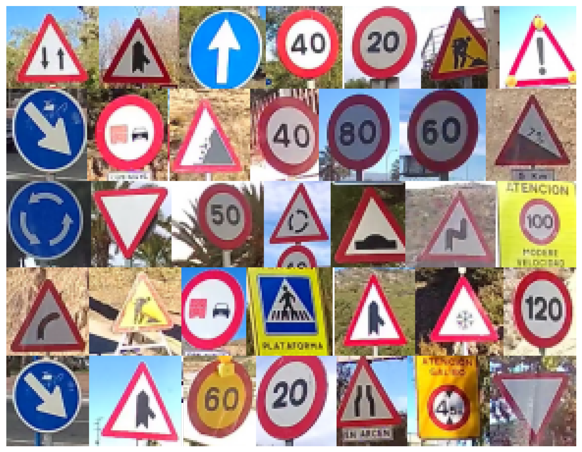
The second group contains 43 different traffic signs (classes) which are most commonly found on European roads. The annotation data includes the class of the object and the bounding box coordinates.
The dataset is a compendium of different publicly available datasets, such as PASCAL VOC [
29] and UDacity [
30], and the remaining data was acquired and annotated from real-life images. From PASCAL VOC, we took only the classes of bicycle, bus, car, motorbike and person, which encompassed 22% of the total dataset. Udacity provided 65% with the classes of bicycle, car, person and traffic light. Then, as we needed to complete the dataset with more objects, we added more images using buses and motorbikes from Internet videos, and bicycles from videos recorded in urban environments and on roads in Alicante (Spain). Finally, we added a small set of traffic lights from our own capture video that accounts for no more than 1%. See
Figure 2 for the distribution of images from the different datasets, and refer to
Table 1 for a later dataset distribution used during the experimentation phase. See
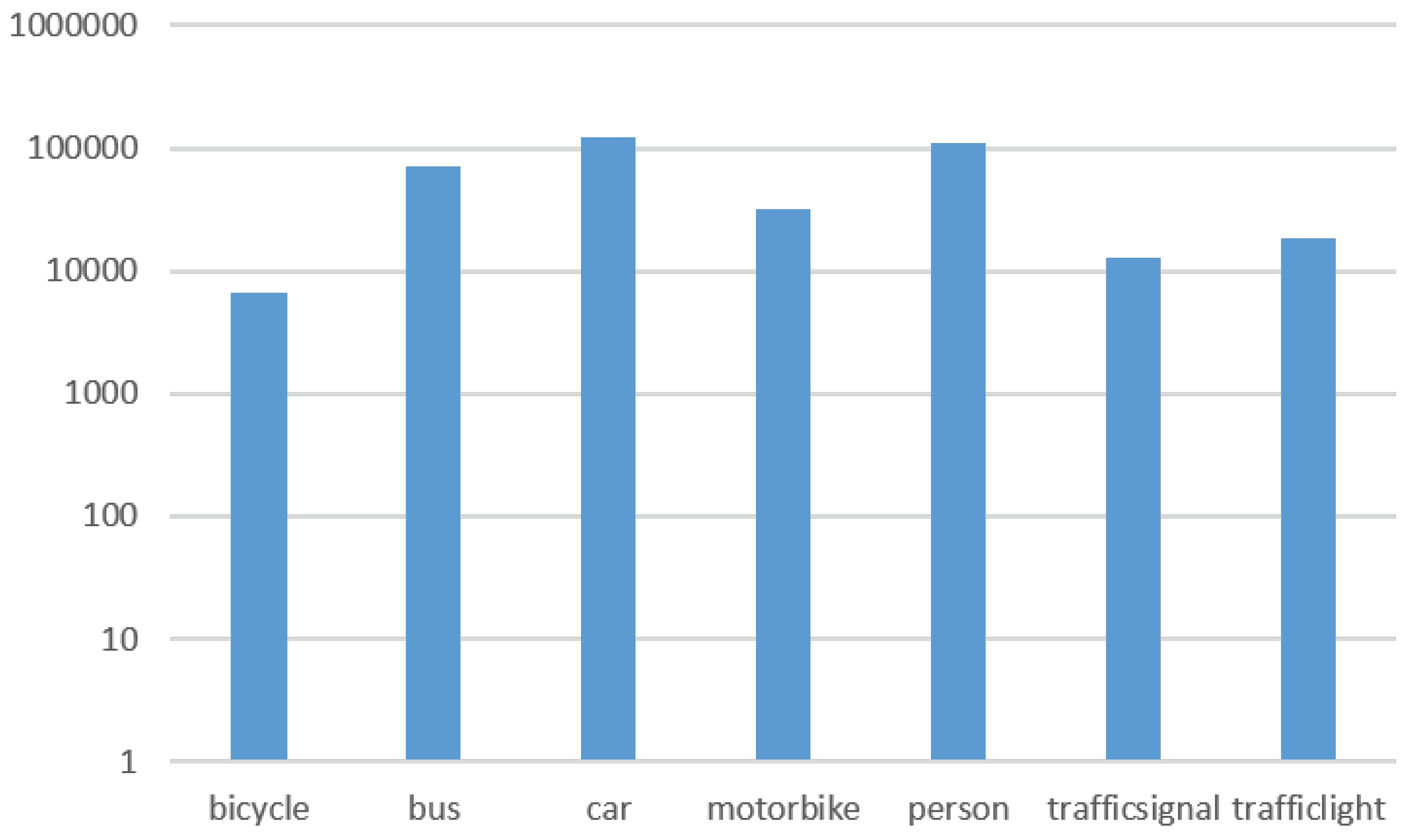
Figure 3 for the initial class distribution.
All the traffic signs found in the dataset (more than 12,000 labeled objects) were annotated within one single class: traffic signal. As explained later, a second dataset containing only traffic signs was created using two publicly available datasets: the GTSRB from the Institut fur Neuroinformatik (Germany) [
31] and another from Linkoping University (Sweden) [
26]. The German dataset contains around 40,000 traffic signs divided unevenly into 43 classes, while the Swedish one has 22 classes and around 6000 traffic signs, all annotated.
The dataset is imbalanced. For the experimentation, we balanced the different classes using data augmentation (rotations, zoom, affine transformation, blurring, etc.) and reduced the three classes with the most elements (car, bus and person).
4. 2D Object Detection and Recognition
4.1. Baseline Method
The main goal of this work was to design a reliable system able to detect the main objects found in a driving situation in any urban or motorway environment. For this purpose, we chose to use a state-of-the-art CNN network to detect the main seven objects within driving environments: cars, motorbikes, people, traffic lights, buses, bicycles and traffic signs.
In order to achieve this, we needed to rely on a robust detection and classification system. It is necessary not just to be able to classify the objects but also to locate them within the scene. A region proposal method was used for this task. Specifically, we built a dataset based on [
19] and their Faster R-CNN work, previously described in
Section 2.
We fine-tuned Faster R-CNN with VGG16 convolutional blocks for this purpose, modifying it to detect eight classes: seven common traffic objects and the background of the scene. Once all the 2D objects were located and identified, it was still necessary to classify all the traffic signs in order for the system to have a robust knowledge of the traffic scene at any given time. Since we grouped all the traffic signs together in a single class, we performed a second step using a fine-tuned CNN to classify the detected traffic signs (43 subclasses). We could have included every single traffic sign as a new class across the rest of the objects, but, as a traffic sign is a class per se, and there are many different types of signs to classify, it seemed obvious and semantically organized to separate them into a different dataset. In practical terms, if we needed to include more types of traffic signs, it would not be necessary to retrain the whole model, but only the traffic sign model with the new traffic sign dataset. The same would apply if we needed to classify different types of cars, brands or models, types of motorbikes, etc.
4.2. Training
The Faster R-CNN was trained using an existing model (PASCAL VOC) based on [
19]. This provided several advantages in certain classes. For instance, the person class, including PASCAL VOC, offered generalization capabilities provided by this general-purpose dataset. The PASCAL VOC dataset includes many people from a variety of angles and sizes, and in different light conditions and poses. In a traffic scene, 99% of persons are normally riding a bicycle or a motorbike or walking alongside a road. Hence, we added this type of object from our recordings to the dataset. The same applies to bicycles and motorbikes. Thus, we also added those objects from our recordings and from the Internet.
The UDacity dataset provided even greater robustness when detecting cars, as all the recordings were acquired from a car’s perspective. UDacity also provides the kind of images and objects one would find in a driving situation: cars and other vehicles from the driving vehicle perspective and angle. This increased the accuracy when detecting cars in our model.
Subsequently, around 375,000 annotated objects from 106,920 images were used for training. The train/validation/test split sizes were 40% for training, 40% for validation and 20% for testing purposes. However, we also evaluated other configurations, such as 60%, 20%, 20% and 50%, 25%, 25%, but the most accurate and robust results were obtained using 40%, 40%, 20%.
We trained the approach for 80,000 iterations, using a learning rate starting at and decreasing it 10 times, after every third of the training process. Momentum was set to and weight decay to .
4.3. Auto-Updated Learning
Once we had a stable and accurate system—let us call it the baseline model—we wanted to test how adding new images increases the accuracy. We call this method the auto-updated learning process. In order to test the auto-updated learning, we composed two automatically annotated datasets with two high-speed cameras: one at high resolution and one at low resolution.
We recorded 7 h 13 m 40 s of 1280 × 720 video at 60 fps in 23 different situations (urban, countryside and motorways). We then converted the video to a lower frame rate. In this case, 10 fps proved to be a good balance between a reasonable number of frames to train without causing many repetitions due to the similarity of sequentially recorded frames.
Recorded sequences were automatically annotated using the baseline model. Once we had this new automatic annotated dataset (see
Figure 4), we added it to the baseline dataset and trained the same architecture used for the baseline model (Faster R-CNN with VGG16 model) again to see how the new model could improve. The baseline model with the new dataset showed an improvement in detecting some of the objects for which it was trained. In a way, the baseline model was learning new features by being trained with new images annotated using the baseline model (see
Table 1). This process was repeated using a different set of images (see
Figure 5) captured with the low-resolution camera, which was able to record at 60 fps but at VGA resolution.
4.4. Traffic Sign Recognition
As previously mentioned, one of the output classes of our trained network is ‘traffic sign’. The CNN network was trained using thousands of images. In order not to just detect but also to classify (traffic sign type) them, we fine-tuned (ImageNet weights) a ResNet50 architecture but now added 43 classes, with these being the most commonly used traffic signs in the European Union. ResNet50 was chosen as one of the latest architectures in the state of the art. To test the model, we used the GTSRB dataset [
31], which also has 43 object classes.
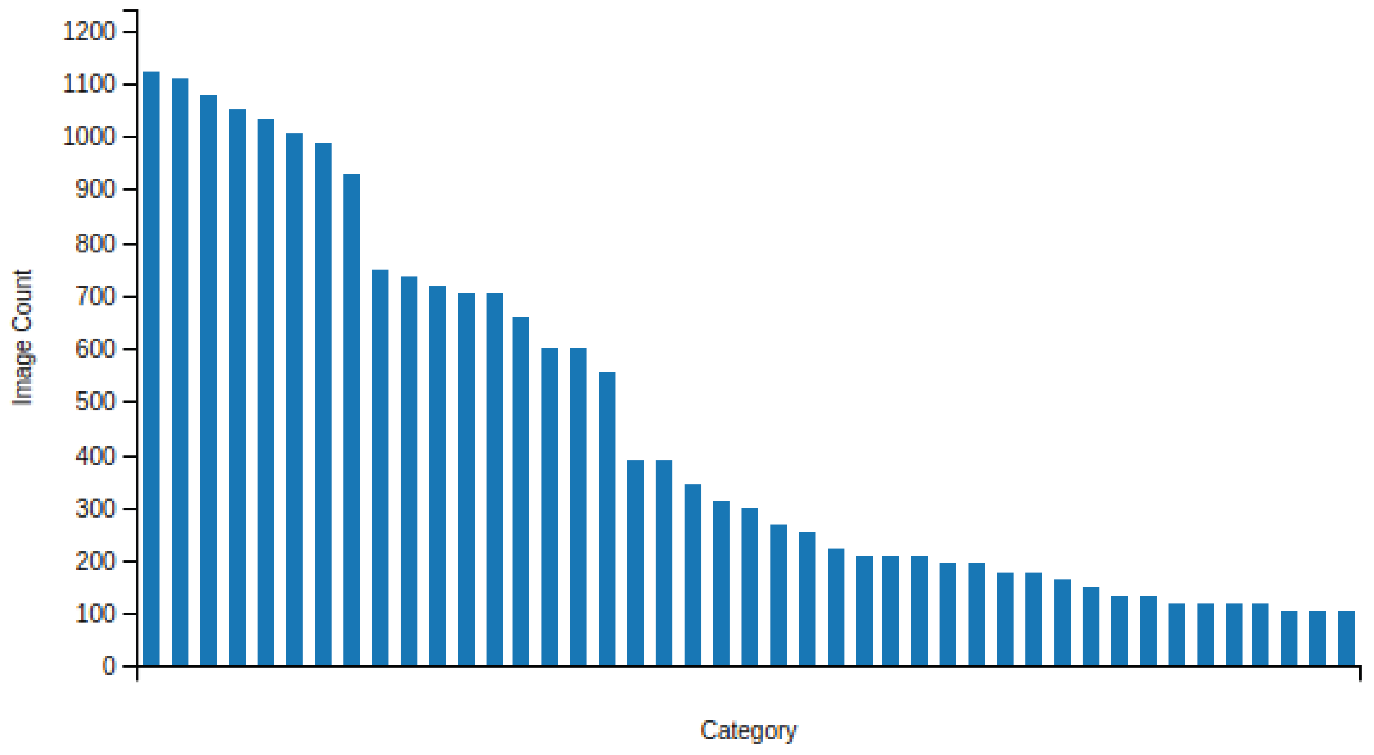
Figure 6 shows the number of images for each traffic sign type (GTSRB dataset). We trained a ResNet50 network using this dataset. The images are square, with sizes that range from 40 to 170 pixels.
Figure 7 shows some traffic sign bounding boxes extracted from the Traffic Signs Dataset [
26]. For training purposes, we implemented data augmentation to compensate categories with a lower number of elements.
5. Experiments
5.1. Setup
We primarily used GPUs from NVIDIA (Titan Xp, GTX 1070 and Quadro P6000) for training the proposed system. At inference time, we also used an NVIDIA GTX 1060.
One of the recording devices we used for acquiring new data was an HD ( resolution) sport camera (H5 Midland) mounted on the front of a vehicle. This camera is able to record video at 60 fps and has a CMOS of 5M pixels and a wide-angle lens of 170°. Moreover, we used a second camera model, the SONY Playstation Eye, which is able to record video at 60 fps (640 × 480 resolution). It uses a VGA CMOS and a wide angle lens of 75°.
A Linux-based system was used along with the Python implementation of the Faster R-CNN [
19], which uses the Caffe Deep Learning framework. Many scripts were modified for our experiments. We fine-tuned the model according to the classes used for the experimentation phase.
We also used the NVIDIA DIGITS 5.1, running the Caffe fork. Finally, for the classification experiments (second step: traffic sign classification), we used the Caffe version of the ResNet50 architecture.
5.2. Performance Evaluation: Urban Object Detection
In this section, we describe all the experiments performed in this work. As a measure of accuracy, we use the mean average precision (mAP), as used in [
19]. We split the dataset into 40% for training, 40% for validation and 20% for testing.
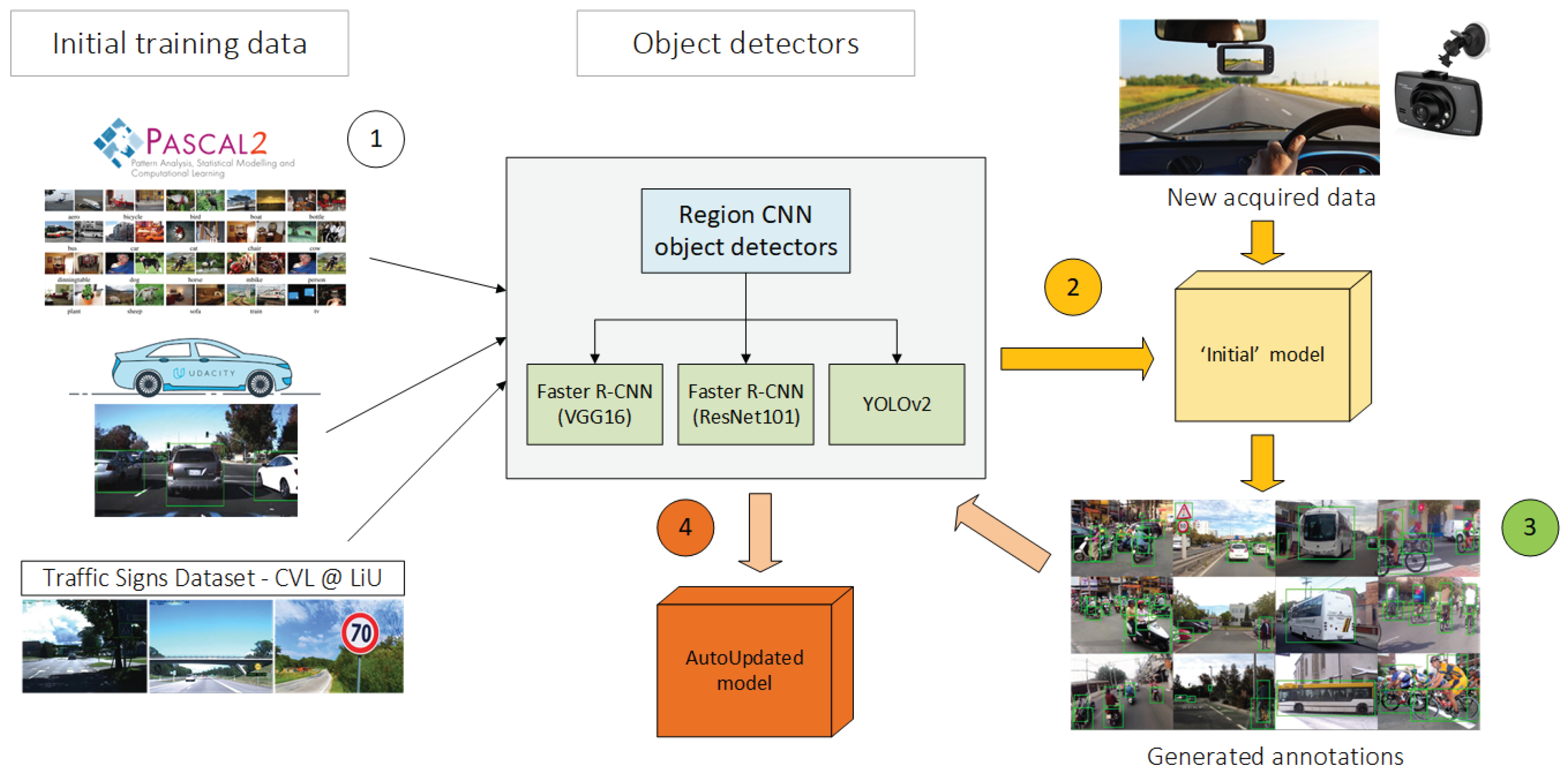
Figure 8 shows an overview of the steps we followed to perform the evaluation of the baseline object detector. It also describes how we trained the ‘Initial’ and ‘AutoUpdated’ versions of the urban object detector model. In step 1, we compiled an initial dataset for urban object detection by filtering particular classes of existing datasets. In step 2, we trained a Faster R-CNN network (VGG16) using the initial version of the dataset. For step 3, using the trained model and new acquired data on real driving scenarios, we automatically annotated new images by using the initial model. In step 4, finally, we retrained the baseline network and other state-of-the-art CNN-based networks (ResNet101 & YOLOv2) using the final version of the dataset (compilation of existing datasets and new recorded data that was automatically annotated).
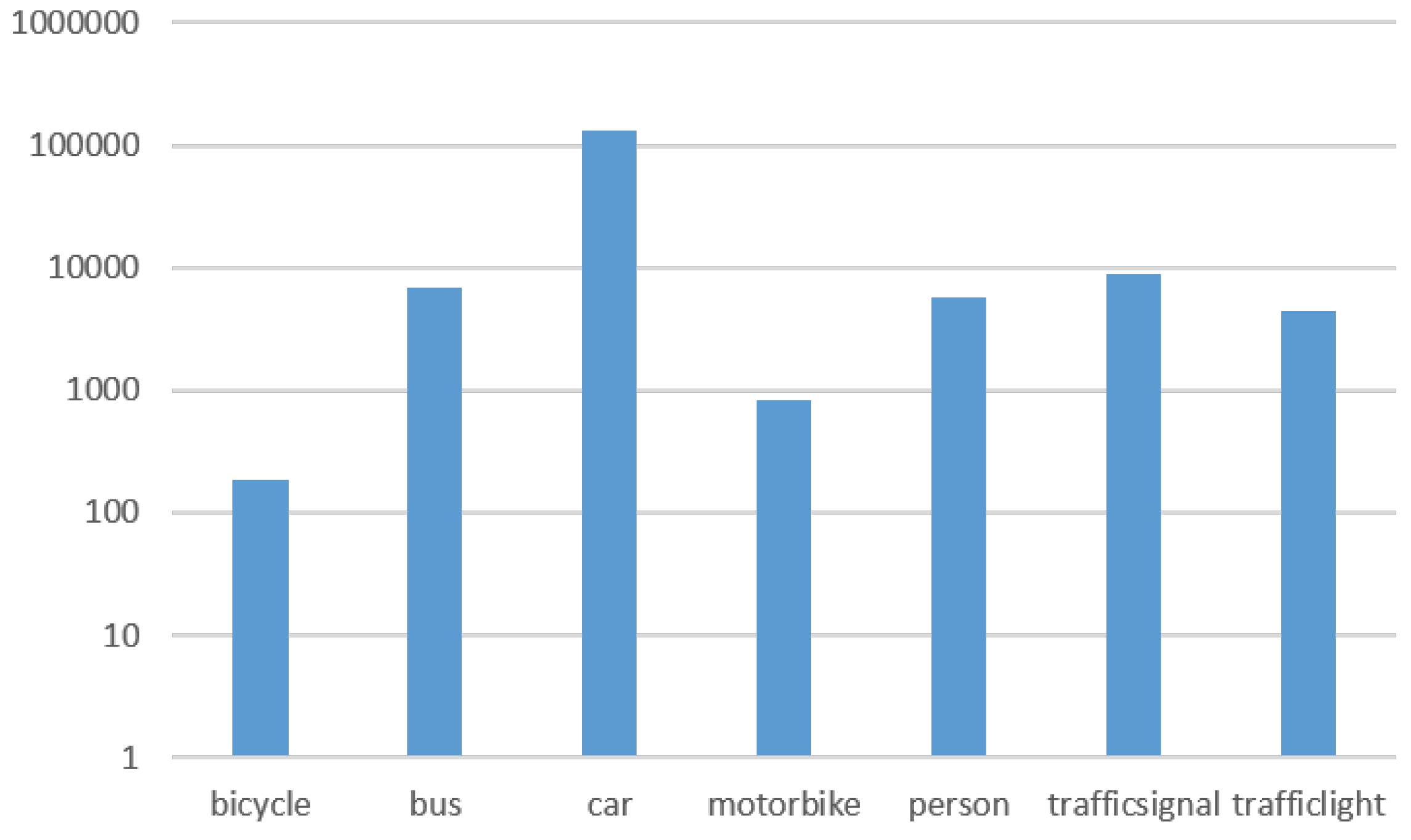
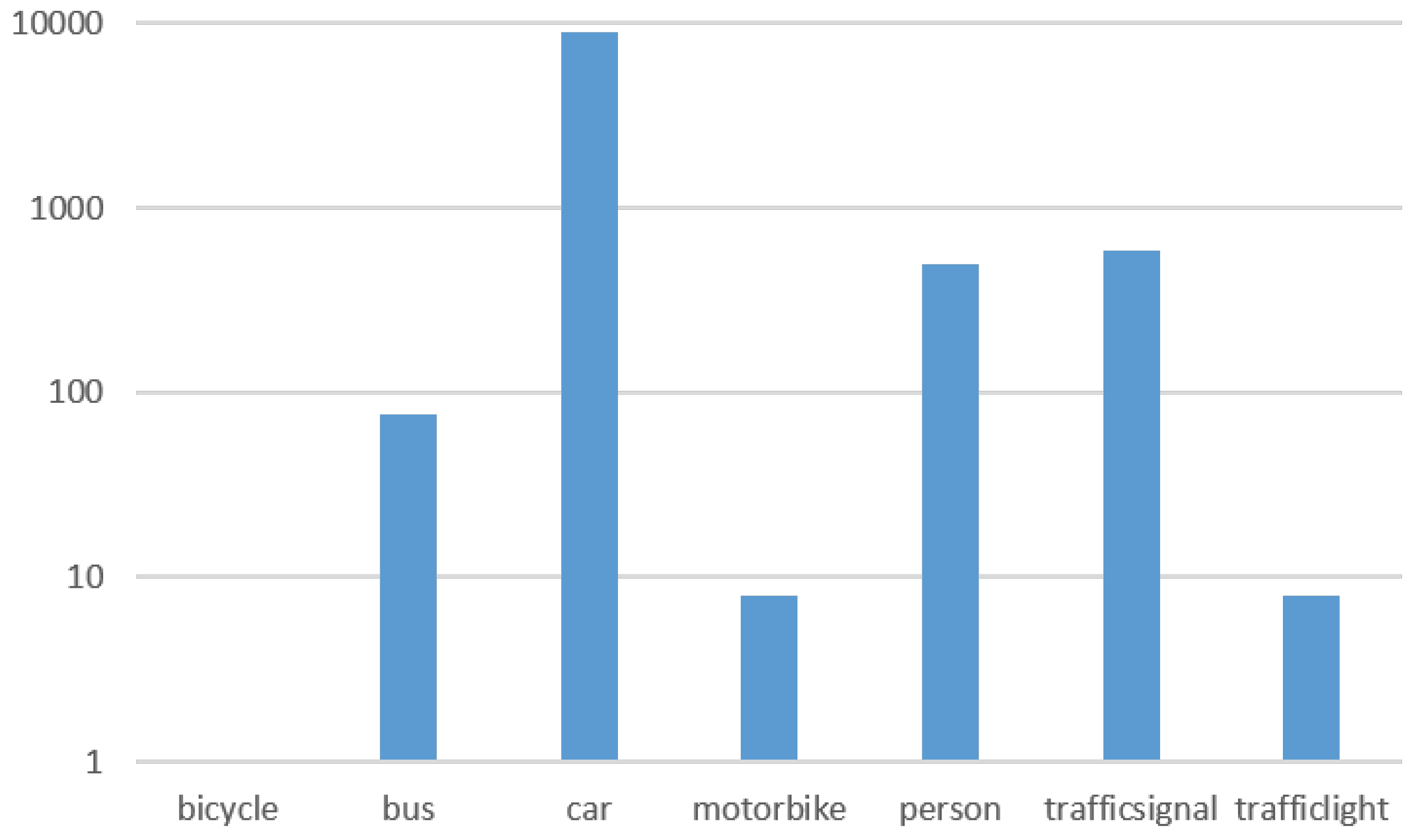
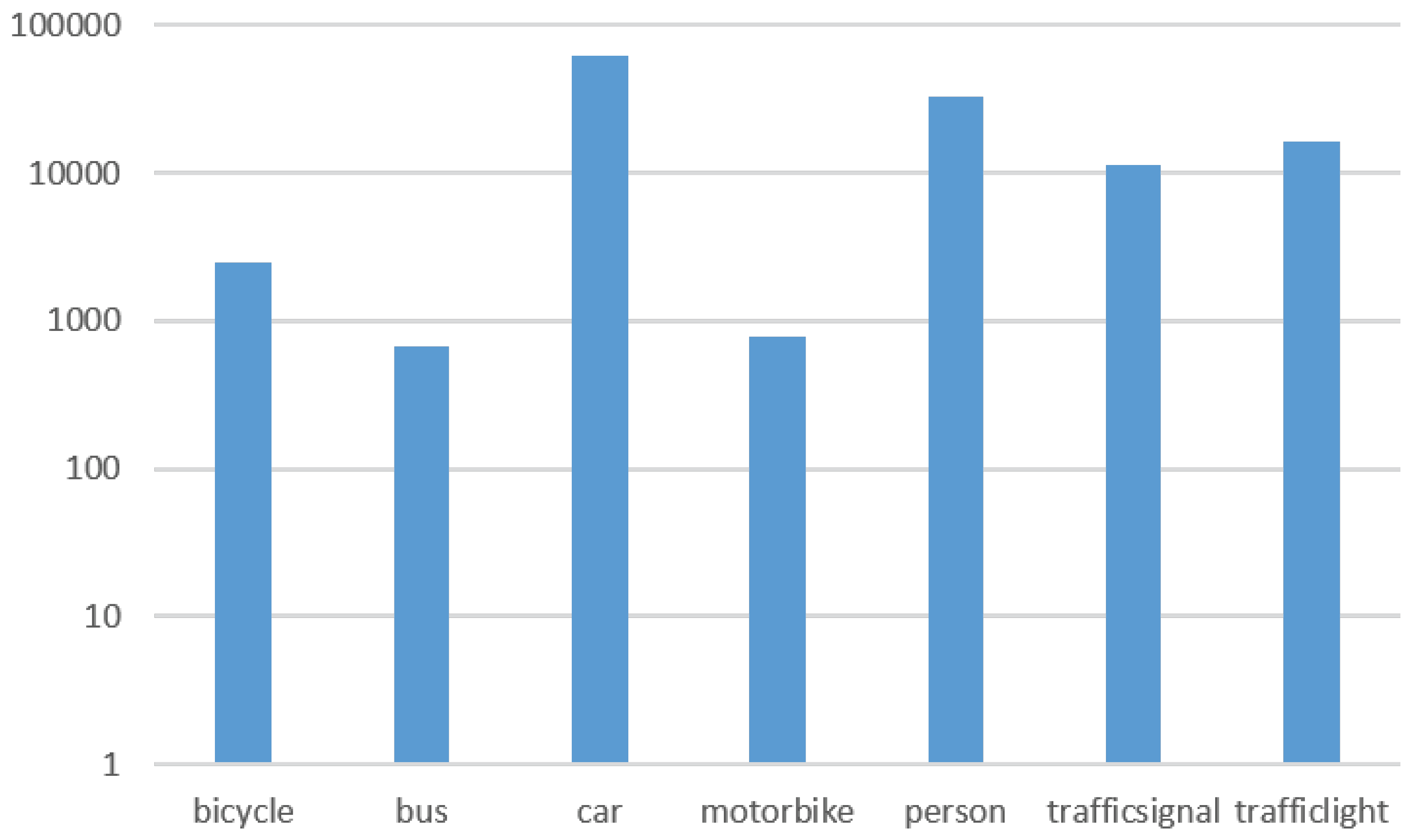
We ended up with a total of 166,139 objects (
Figure 9). For this experiment and the subsequent ones, we used the Faster R-CNN architecture, using VGG16 convolutional blocks [
18], which is more computationally costly (slower training/inference than YOLOv2) but provides greater accuracy.
We noticed that the mAP for the traffic light class was not as accurate as with the other classes, even using 10% of the total dataset (16,564 traffic lights, see
Figure 9). Many of the bounding boxes for traffic lights were very small (fewer than 240 squared pixels), so we decided to filter out the very small ones, as they would provide no practical information in a driving situation because, with the bounding box being so small, the traffic lights would be extremely far away from the vehicle.
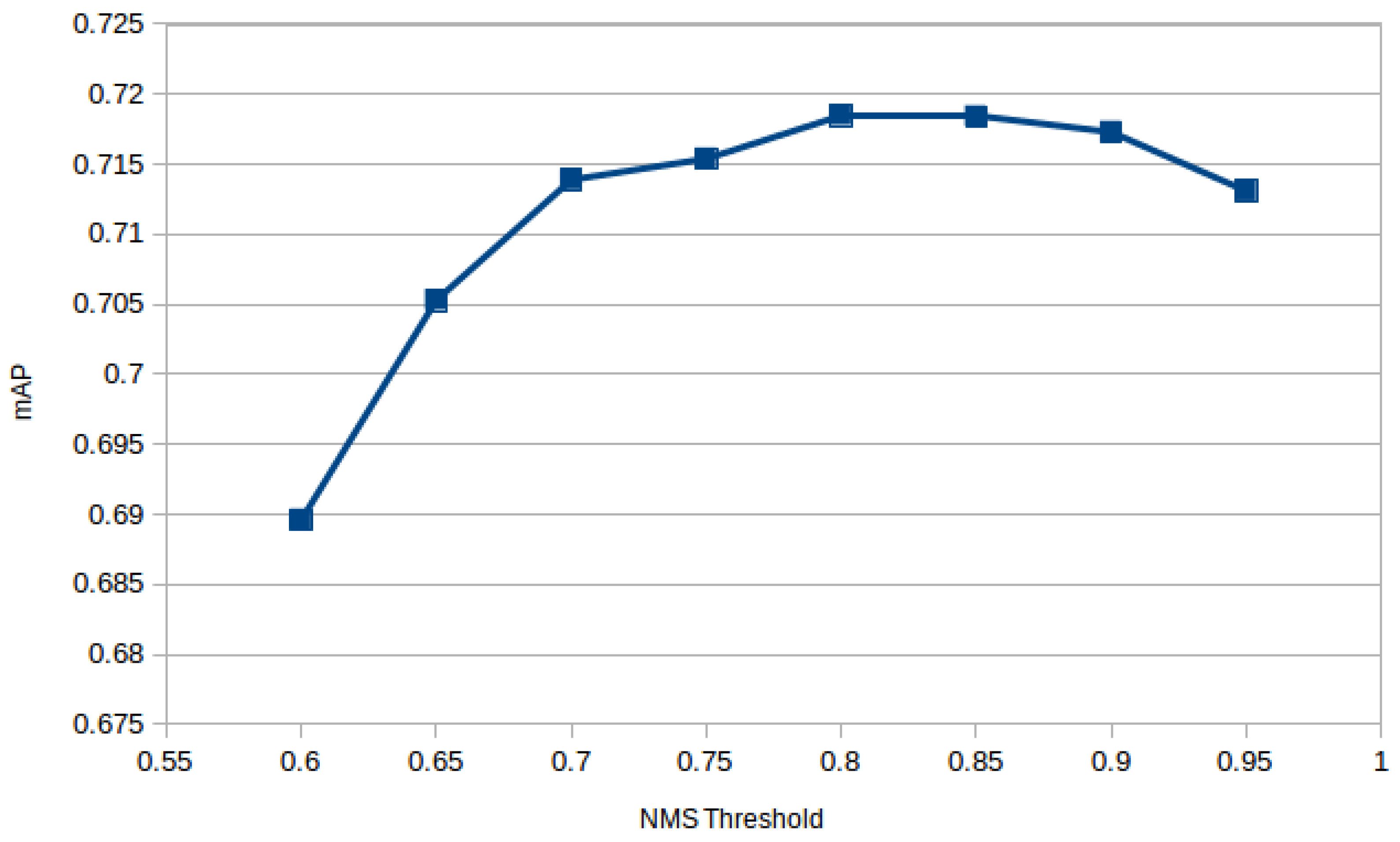
In [
19], the author used a non-maximum suppression (NMS) threshold for the removal of candidate regions, setting a fixed threshold of
. We tried several thresholds to select the correct one. The best NMS threshold was
(see
Figure 10). We trained the baseline model for 70,000 iterations, starting with a learning rate of 0.001. The results are shown in
Table 1, Baseline method.
We observed that the detection accuracy for bicycles and motorbikes was not as high as for other classes, such as cars or people. Furthermore, the distribution of bicycle and motorbike objects in the dataset was also too low in comparison with the other classes. Buses were also too low, and many buses in real-life tests were not detected. So, we decided to add more of these objects (buses, bicycles and motorbikes) to the dataset, again using an auto-updated technique. We annotated 7 h of recordings (10 fps videos, recorded with the H5 camera). From those labeled images, we increased the number of buses, bicycles and motorbikes (and the other classes such as cars, people, traffic signs were also shown in the new images).
We then trained for
iterations. We implemented data augmentation as explained before, thus ensuring all the classes were evenly included in the training and validation set, achieving a mAP of
.
Table 1 shows the results for the different R-CNN architectures that we evaluated. The first column shows the mean AP score for the baseline method (Faster R-CNN with VGG) using the ‘initial’ dataset (compilation of images from existing datasets). The second column, ‘AutoUpdated’, shows the mean AP score of the baseline method trained using the final version of the dataset (compilation of initial images and new recorded sequences). The new recorded sequences were annotated by using the initial model. Finally,
Table 1 shows the mean AP score for the YOLOv2 and Faster R-CNN with ResNet101 architectures. Both of these networks were trained using the final version of the proposed dataset (AutoUpdated). As we can see, using ResNet101 convolutional blocks for object detection produces slightly worse results compared to using VGG blocks. Moreover, we show how YOLOv2 produces a lower mean AP score compared to the Faster R-CNN methods; however, YOLOv2 has also a lower runtime, which makes it suitable for real-time systems.
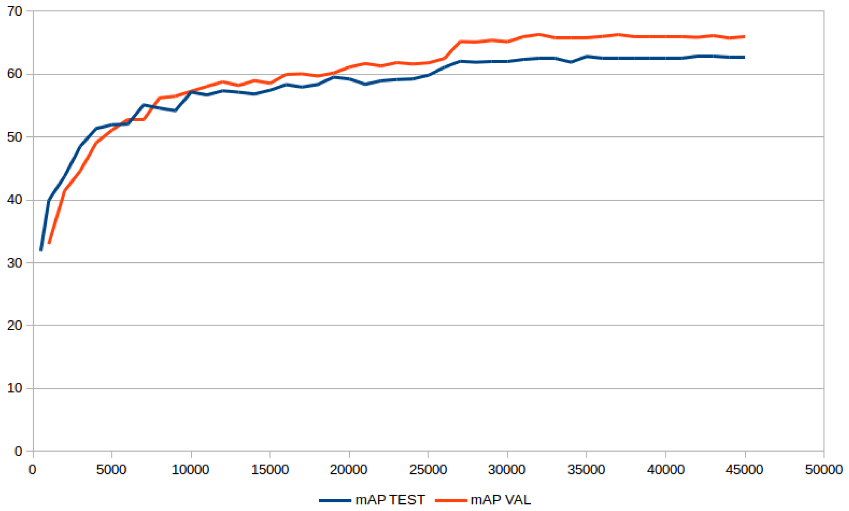
As the goal of this work is to deploy the developed system in an embedded system (like a Jetson card or FPGA), we need a fast implementation of the object detection component. Therefore, we evaluated the Darknet version of YOLOv2 [
20] in our seven-class dataset. We applied a learning rate of
and trained for 45,000 iterations, with a momentum of
and decay of
. We also achieved good results with our dataset, achieving a mAP of
in the test set. After approximately the 27,000th iteration, the mAP stabilized, achieving no further increase in accuracy (see mAP evolution in
Figure 11). See
Table 1, YOLOv2, for results.
5.3. Additional Test, Processing a Mix of Real-Life Clips Acquired in Various Urban Environments
After observing the mAP results within the previous experiments, we wanted to test whether our latest model could improve in terms of detection accuracy even though the mAP slightly decreased due to the lack of balance in terms of the number of annotations per class.
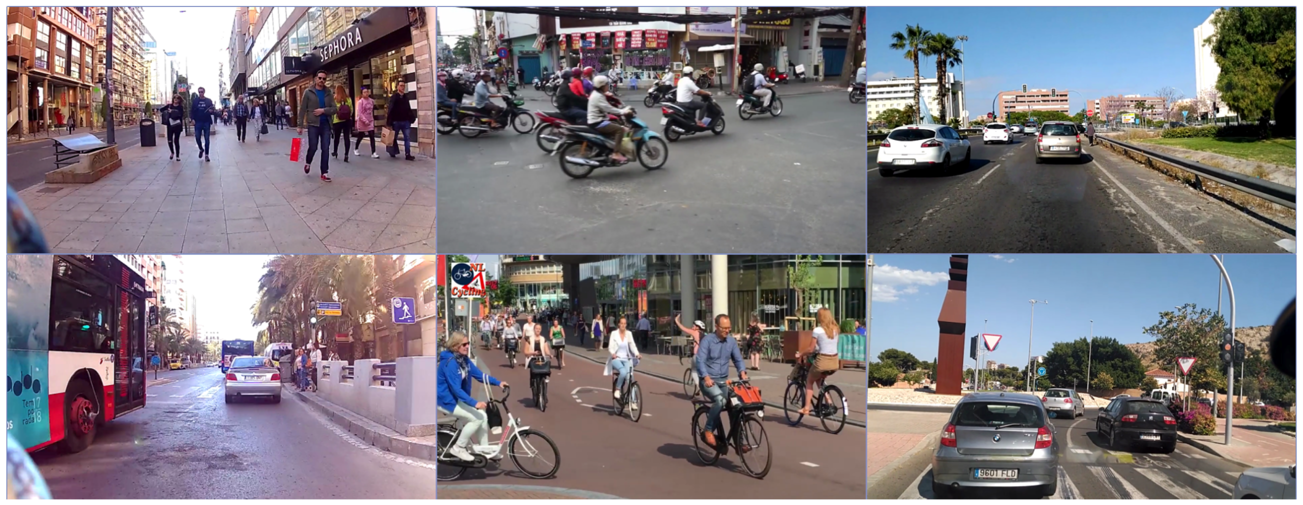
We recorded real-life videos of scenes containing many of the urban objects defined in the classes of the proposed dataset. The actual video has 8992 frames, and was mainly recorded in very busy urban environments (see
Figure 12). The video does not represent a ground truth of detected objects, but it gave us information on how much better (in terms of number of detected objects) one CNN model is with respect to the others. It also provides a visual confirmation of the mAP coefficients measured earlier. After detecting all the objects in the scenes and computing various statistics for the processed video, we concluded that the auto-updated training strategy improved the accuracy when detecting objects (see
Table 2). The accuracy was not greater in terms of mAP, but the number of correct bounding boxes that were predicted increased compared to previous experiments. Moreover, in some cases, the improved model was able to detect bounding boxes that were not previously detected (decreased the number of false negative detections).
5.4. Traffic Sign Classification
In the last years, CNNs have surpassed most traditional methods, achieving a 99% classification accuracy on publicly available datasets for traffic sign recognition [
32]. In order to complete the creation of a more complete urban object localization system, we focused on the traffic sign classification task. We needed to be able not just to detect a traffic sign, but also to classify it. We chose a ResNet50 architecture for this task due to its proven speed and accuracy for classification tasks [
16,
33]. In this work, we fine-tuned the original model, which was trained using the ImageNet dataset, using the German traffic dataset (GTSRB) for evaluation purposes. The GTSRB dataset contains 39,495 images of 43 different traffic signs (see
Figure 6 and
Figure 7). Additionally, we created a new Spanish traffic sign dataset with 3300 images divided into 45 traffic signs. This was acquired from the previously presented dataset (
Section 3) by automatically cropping the resulting detected traffic signs using our previous Faster R-CNN baseline model.
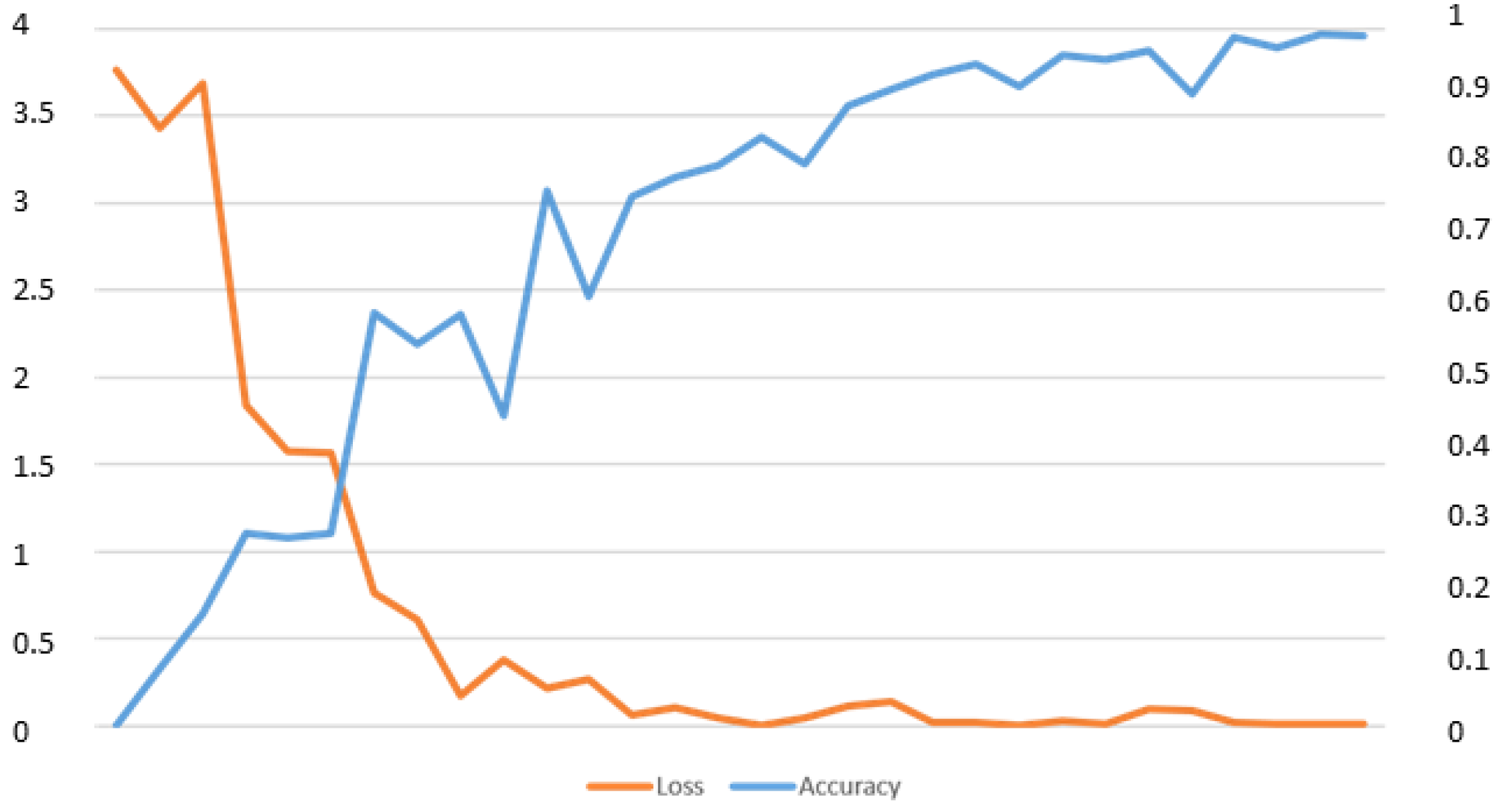
We trained for
iterations, using a learning rate starting at
with a polynomial decay gamma value of
and weight decay of
. The dataset was split as follows: 50% for training, 25% for validation and 25% for testing. It obtained 98.09% accuracy on the test set (choosing the class with the greatest probability) and 99.76% accuracy when performing a vote using the top five predicted classes. As a final test, we added 100% of the Spanish dataset to the GTSRB and applied the same distribution. Testing against the ground truth resulted in 99.7% accuracy on Top1 and 99.9% on Top5 (see accuracy and loss in
Figure 13).
5.5. Discussion
While creating this dataset, we discovered that the amount and variety of data used for training a CNN are crucial for the accuracy of our application to unseen data. As we added more data from different sources and domains, with different scenarios and backgrounds, we saw that we were able to decrease the generalization error (unseen data). However, in some of the experiments, we also realized that, due to the increase in the diversity of our training data sources, the system was performing worse on certain classes due to imbalanced data. To address this problem, we had to capture new data focusing on creating new annotations for imbalanced classes. After training a new model considering these two factors, we were able to increase the accuracy of the trained model and also reduce its generalization error.
6. Detection and Tracking
In this section, we explain how tracking objects in a video feed can benefit from the detection process of a region CNN.
6.1. Motivation
The main goal of an urban R-CNN model would be to implement such a system in a real-life vehicle, in a real traffic environment. As we know, such systems require great GPU performance; most (probably small) embedded systems would be more realistic final hardware to implement such a network, so a good way to accelerate the detection process using software is needed. Consequently, we tracked the detected object in certain ways in order to alleviate the GPU for such work.
6.2. Strategy
The strategy to follow in the detection-tracking mix would be to first detect the objects with an R-CNN, which should occur quickly enough to work in small hardware, then track the objects either until they are lost or until the reliability of the tracker is found to be diminished and there is insufficient confidence in the localization of the object detected in the first place.
We analyzed several tracking algorithms: Correlation tracker [
34], Deep sort [
35], Boosting [
36], Mil [
37], KCF [
38], TLD [
39], MedianFlow [
40] and Mosse [
41].
All those algorithms were evaluated in three different GPUs from an NVIDIA 940M, a 1050 Ti and a 1080. We tested them for speed, accuracy and robustness. Moreover, we studied the point at which it is best to relaunch our R-CNN detector to detect the objects again. In some cases, launching the R-CNN every n frames was a good solution; in others, launching as soon as the tracker lost the object also achieved good results. Hence, a balance of these two strategies proved to be the best option for real-time processing given a limited computing budget.
Some algorithms are good for relocating the tracked object after a partial occlusion, but, as this is not strictly relevant to our purpose, we did not focus on this feature.
Additionally, the goal of the detection-tracking bundle is to prove that hungry GPU processes, such as R-CNNs, can benefit from tracking techniques, not to present an exhaustive study about tracking algorithms.
We chose three of the nine algorithms tested: KCF, MedianFlow and Mosse. These were found to be quite fast with reasonably good accuracy in urban environments.
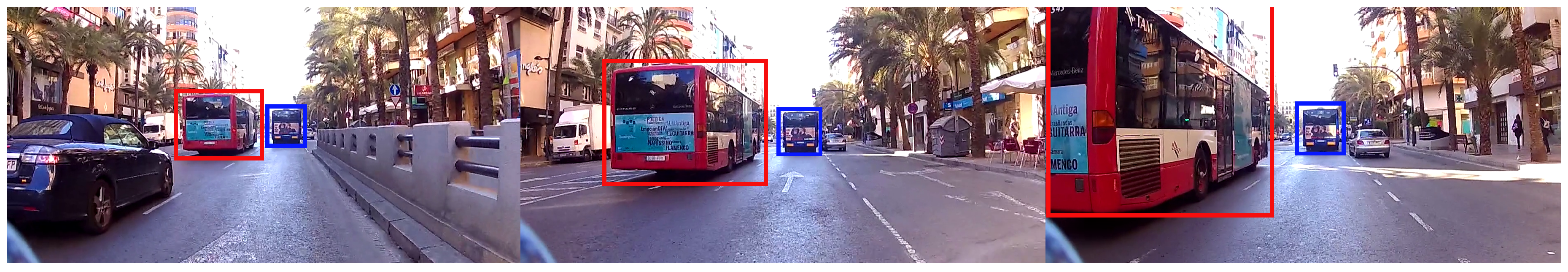
Tracking objects in a traffic environment from a moving car has a particular drawback related to tracking objects in the outside edges of the camera view, such as parked cars, pedestrians or overtaken vehicles such as cars or buses. These objects can very rapidly increment their size and location in the scene, and most trackers do not perform well with such large and fast variations. However, objects moving beside or in front of the car can be tracked for a long time. An example of this can be seen in
Figure 14.
6.3. Experiment: Detecting with YOLOv2 Every n Frames.
Although Faster R-CNN provided better mAP than YOLOv2, we chose the latter for our experiments. This is due to YOLOv2 having a shorter execution time, and this system is intended to be embedded in devices such as the Jetson TX2 from NVIDIA.
The first experiment was based on detecting objects in an urban environment video with
pixels in RGB format at 30 fps. With our seven-class urban dataset, we used YOLOv2 to detect objects (cars, buses, pedestrians, etc.) and let the Mosse tracker follow them for
n frames. As can be seen in
Table 3, the longer the period to relaunch YOLOv2, the faster the algorithm. The goal of this experiment was to prove that YOLOv2 detection would benefit from intermediate tracking and to determine how long a tracker was a beneficial option (
Figure 15).
6.4. Experiment: Urban and Motorway Environments
For these tracking algorithms, we needed to know how much the tracker would help the YOLOv2 R-CNN detection.
We set two traffic videos of roughly the same length, about 4 min 20 s: one in a busy urban environment and the other in a motorway environment. Videos were 1280 × 738 at 30 fps. We launched YOLOv2 just every 30 frames, and in the rest of the frames, the tracker was in charge of locating the objects. We measured the average frames per second, comparing the video using just YOLOv2 with the same video using no tracking help at all. We also measured the percentage (based on number of frames) where YOLOv2 was used. We tested the three tracking algorithms, the results of which are presented in
Table 4. Note that frames with no objects in the scene were not taken into account for the percentage results.
It can be seen that the use of GPU (YOLOv2 usage) can be dramatically reduced by between 10% and 14% when using a tracking algorithm, accelerating the calculation process as a whole. Consequently, the average speed (in fps) can be increased.
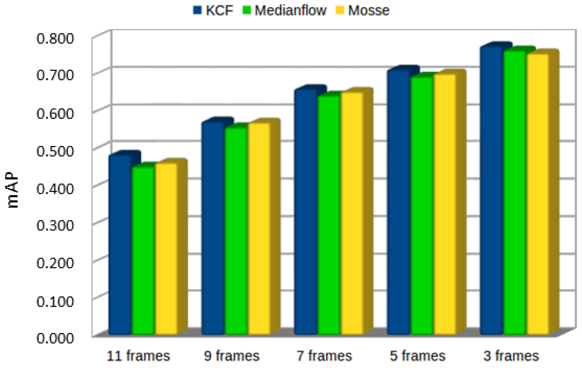
6.5. Experiment: mAP Accuracy in Trackers
Finally, we tested how accurate these tracking algorithms were and for how long the tracking algorithm could keep track of the detected object, with the tracked object being sufficiently reliable or as reliable as the YOLOv2 detection.
We set the ground truth of all bounding boxes detected by YOLOv2 in every single frame (8117 frames). We then let the tracking algorithm locate these objects for n frames and compared the bounding boxes produced by the tracking algorithm with the YOLOv2 ground truth in order to have a mAP. As can be seen in
Figure 15, the tracking location is reasonably accurate until the 10th frame but, after that, the mAP is less than
. It is also noticeable that KCF is slightly more accurate than the other two trackers.
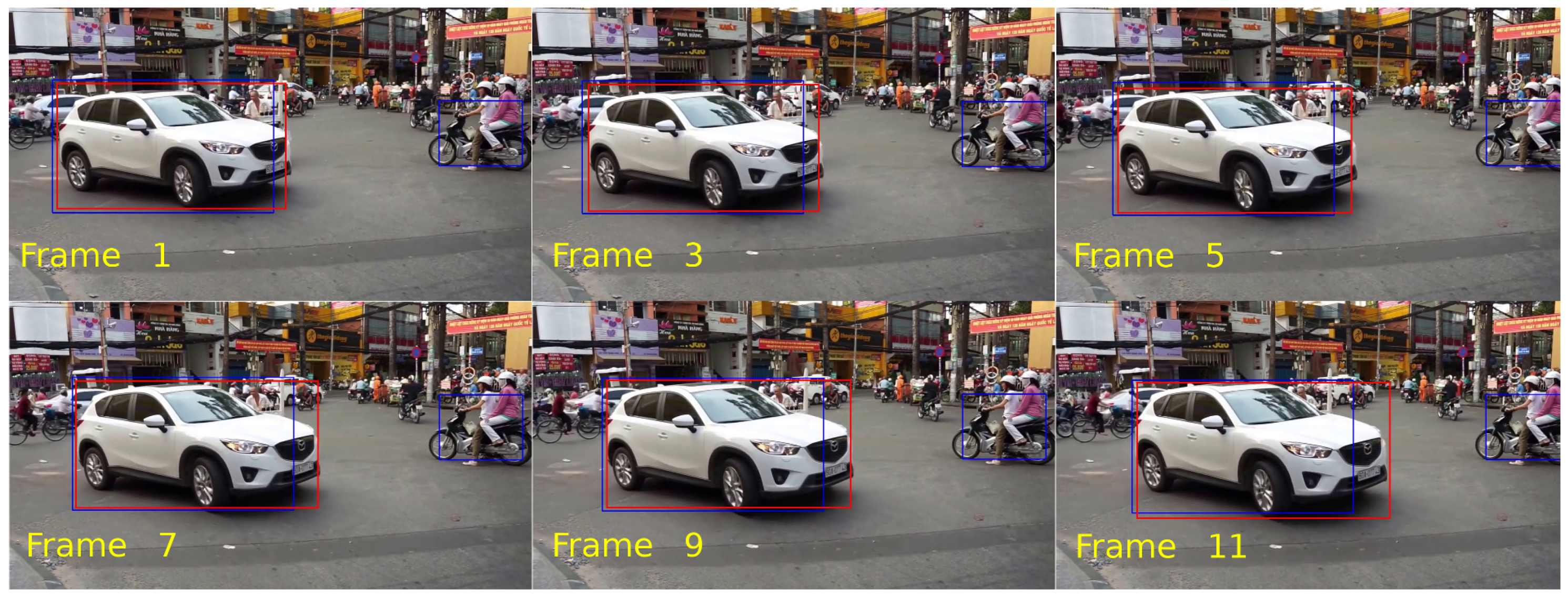
Figure 16 shows examples of how accurate the trackers are in relation to the number of frames between YOLOv2 detections.
Figure 17 shows that the tracking of detected bounding boxes differed between YOLOv2 detection and that, after the 11th, this can be noted visually.
We can conclude that tracking definitely accelerates the detection process as a whole. In
Table 4, the increase in speed obtained in this experiment by applying any tracking algorithm can be seen. For instance, in an urban environment, using a reasonably low GPU, such as an NVIDIA 1050 TI, we go from
fps using only YOLOv2 to
fps by adding a MedianFlow tracker, which represents an increase of over 100% in calculation speed.
7. Conclusions
In this work, we present a new dataset for urban object localization, which is a compilation of new and existing data. It includes annotations not just for common moving objects, such as cars, pedestrians, bicycles, etc., but also for static traffic signs and traffic lights.
We trained a state-of-the-art Region-based CNN, Faster R-CNN architecture, and proved how well this dataset can be used for real-life traffic situations, such as urban and motorway scenarios, achieving a mean average precision accuracy of . Moreover, by retraining the proposed architecture following an auto-updated strategy, we demonstrated how the proposed R-CNN network improved its accuracy (fewer number of false negatives) in real-life driving situations. Additionally, we evaluated other state-of-the-art detectors, such as Faster R-CNN with ResNet101 convolutional blocks and YOLOv2. From these experiments, we concluded that Faster R-CNN with ResNet101 performed very similar to the proposed baseline, and YOLOv2 achieved lower mean AP scores but it considerably improved overall performance (runtime).
We also proved that tracking techniques can noticeably improve R-CNN object detection (YOLOv2) and its efficiency by balancing the use of both, detection and tracking, without losing accuracy.
As a future work, we plan to merge the existing traffic sign datasets used in this project. We plan to repeat the same process followed in this study and extend these datasets using an auto-updated strategy.


