Article

Metaheuristic Regression Equations for Split-Ring Resonator Using Time-Varying Particle Swarm Optimization Algorithm

Department of Electrical Engineering, Faculty of Engineering and Technology, HITEC University, Taxila 47080, Pakistan
*
Author to whom correspondence should be addressed.
Electronics 2018, 7(11), 300; https://doi.org/10.3390/electronics7110300
Submission received: 5 October 2018 / Revised: 24 October 2018 / Accepted: 1 November 2018 / Published: 5 November 2018
(This article belongs to the Section Microwave and Wireless Communications)

Abstract

:
This article presents a new technique for determining accurate values of resonant frequency and quality factor pertaining to the split-ring resonator. Different conducting shield materials have been used around a copper split-ring. The split-ring has been designed to operate at about 2.1 GHz. Various equations were worked out earlier to determine the values of resonant frequency and quality factor. However, these equations yielded different solutions. Therefore, simulations were used to obtain the values of the resonant frequency and quality factor of the split-ring resonator with different five-shield materials, using High-Frequency Structure Simulator (HFSS) software. In this work, a novel method has been introduced for obtaining values of resonant frequency which provides results with negligible error. An optimal technique, namely time-varying particle swarm optimization (TVPSO), was then performed to obtain two sets of equations for resonant frequency and quality factor. The two sets of equations, optimized using TVPSO, were compared for their effectiveness in matching the actual frequency and quality factor for each of the five materials. It was found that the TVPSO was significant in achieving the frequency and quality factor regression equation to accurately resemble the actual values portrayed by the low mean absolute error.

1. Introduction

The split-ring resonator (SRR) is a structure that has utility in various microwave applications [1,2,3,4]. This structure (in different configurations) has been used in both planar and non-planar forms. These applications include material characterization [5], compositional analysis [6], food grading [4,7], bio-medical applications [2,3], meta-materials [8], quality control etc., in the 1–5 GHz range. The SRR is characterized by ease of fabrication, low cost, moderate quality (Q) factor, low noise interference [9] etc. It comprises a metallic ring with one or more longitudinal gap(s) and generally enclosed in a metallic shield [10,11,12] for better performance [13]. This work is particularly focused on non-planar SRR. Besides SRR, there are also other resonator topologies which have been presented in the literature [14,15]. A single-gap SRR is shown in Figure 1 [16].
The resonant frequency and Q-factor are important parameters of the SRR which are worked out to determine its applicability [17] in different circumstances. A longitudinal gap of SRR ‘t’ represents capacitance, while the single turn represents inductance of the structure. The resonant frequency is generally obtained on the basis of these quantities, besides the dimensions of the split-ring and shield. This quantity has been worked out by numerous researchers [11,12,13,18]. One such equation worked out for obtaining the value of resonant frequency while considering the fringing field and shield effects is given below [19]:
f 0 = c 2 π r 0 t π W 1 + r 0 2 R 0 2 ( r 0 + W ) 2 1 + Δ Z Z 1 + Δ W W
where t, W, Z, r 0 , R 0 are different dimensions of SRR and shown in Figure 1. ΔZ is the equivalent length extension due to the magnetic fringe fields at two ends of the resonator, whereas ΔW is the equivalent length extension due to the electric fringe fields at two ends of the resonator [16]. These are calculated as ΔZ = 0.18 R 0 , ΔW = 3.0t. The Q-factor of SRR is an important figure of merit and is worked out on the basis of material property and dimensions of split-ring and shield. One such equation for the Q-factor while considering ohmic losses on walls of resonator and shield, effects of fringing field and shield effects is given below [19]:
Q S = r 0 δ ( 1 + r 0 2 R 0 2 ( r 0 + W ) 2 ) ( 1 + Δ Z Z ) 1 + ( 1 + W r 0 + R 0 r 0 + R 0 2 3.8 Z r 0 ) ( r 0 2 R 0 2 ( r 0 + W ) 2 ) 2
where δ is skin depth of resonator material. However, the above requires correction due to conductor loss of the capacitor gap and is given as [16]:
Q C = 1.7 × 10 5 t f 0 3 / 2 ε 0 W 2 ( 1 + Δ W W )
Overall Q-factor is, therefore, worked out as:
1 Q = 1 Q S + 1 Q C
Utilization of the resonance technique for obtaining resonant frequency and Q-factor is a well-established method and has been in use for performing compositional analysis, permittivity sensing, biomedical electron paramagnetic resonance (EPR), etc. [1,3,6,20,21]. Hence, obtaining the exact/accurate value of parameters is essential for optimum utilization of components/devices. For obtaining resonant frequency and Q-factor of the split-ring resonator, numerous models have been formulated [13,18,19]. A comparison of SRR models [13] shows that at times large errors were obtained. So, there exists a need to determine these values using a numerical approach. Basing on these observations, regression equations were obtained [9]. These equations yielded values that are relatively accurate. Since Equations (1)–(4) mentioned above and other similar models only provide approximate values [13], they may provide inaccurate information. Inaccurate values obtained through these models may lead to incorrect design and a wastage of time and effort. Simulation results are also not accurate as mentioned in earlier work [22]. The difference in the two values is mainly due to changes in material properties during machining work, small inaccuracies in fabrication, besides other reasons. However, HFSS simulation yields results better than the mentioned models. So, simulation values can be utilized with a certain degree of confidence. Due to this reason, HFSS [23] simulation has been utilized for this work. The default settings of HFSS have mostly been utilized so that these have equal effects on the obtained values. Regression equations were obtained, with the help of simulated results obtained using MINITAB software [24] to determine values of resonant frequency and Q-factor with high accuracy for different shield material around a copper ring [9]. Optimization is required to use a requisite object in its optimal way. Recently, metaheuristic optimization techniques have found tremendous applications in various fields of engineering and science [25,26]. Particle swarm optimization (PSO) being one of the most used metaheuristic algorithms, has played a substantial role in various problems. Particular to communication and electronics fields, PSO has many applications [27,28,29]. This optimization algorithm yields solutions using the iterative method and tries to improve the successive result with regard to a given measure of quality (objective function). It uses predefined data, which are dubbed particles, and these particles are moved around in the search-space over the particle’s position and velocity to yield solutions.
In this work, a novel method has been introduced for obtaining the values of resonant frequency and Q-factor, which provides results with negligible errors. Two sets of equations for resonant frequency and Q-factor have been obtained for different shield materials around a copper ring, as discussed above. Coefficients of the two sets of equations have been optimized by a variant of standard PSO, namely time-varying particle swarm optimization (TVPSO) which has been effective in finding global solutions to many engineering problems [30,31], by formulating an optimization problem using a minimizing objective function. Comparison of the results is presented for validation and usability of the presented technique.

2. Problem Formulation and Methodology

The resonant frequency and Q-factor of SRR are dependent upon critical dimensions besides material and other properties. Important material properties which affect the values of these parameters include bulk conductivity, relative permeability and mass density of both the split-ring and shield material [9]. Important properties of the shield materials are given in Table 1 [9]. As per guidance available in earlier research [1,10,11], high conductivity is a necessity for a split-ring, so copper has been utilized in this work to design the split-ring. The shield has been designed using aluminum (AL), brass (BR) [21], stainless steel (SS), cast iron (CI), and tin (SN). These have been previously utilized in an earlier work [9].
Equations of the resonant frequency and Q-factor of SRR can be obtained using data. Data can be obtained with the help of simulations. For this purpose, five base-design SRR models were formulated using HFSS, each with a shield of different material. Design parameters of the base design SRR are produced in Table 2. A square cross-section of the ring was developed so that magnetic and electric fringing effects remain uniform in vertical and horizontal directions. A HFSS simulation model comprising of SRR enclosed in a shield, designed for this work, is shown in Figure 2. Five sets of values pertaining to resonant frequency and Q-factor for the base design SRR were obtained. For studying the effects of variations in shield dimensions on the resonant frequency and Q-factor pertaining to each of these, dimensional parameters had to be varied within allowable limits. These ranges were obtained as per the guidelines worked out by earlier researchers. The range over which parameters were to be varied are tabulated in Table 3 [9]. It can be observed that each of the parameters, namely height of shield ‘H’, the inner radius of shield ‘R0’ and thickness of shield ‘T’, had 5 values. So for each shield material, 125 (5 × 5 × 5) solutions were required. The grand total of solutions for all SRRs with shield, of five defined materials, was 625 solutions.
The effects of variations in geometrical dimensions of the shield on the resonant frequency and Q-factor using full factorial method could be studied with the help of a full factorial experiment. In the full factorial experiment, all combinations of variable levels are included to find solutions [32]. In this case, 625 experiments had to be designed because three variables used five levels of values for each shield material, as discussed above. In order to reduce the number of experiments without losing accuracy in the results, the Design of experiment Taguchi approach [33] was adopted. The Taguchi method defines two types of factors, namely control factors and noise factors. An inner design constructed over the control factors finds optimal settings. An outer design over the noise factors looks at how the response behaves for a wide range of noise conditions. The experiment is performed on all combinations of the inner and outer design runs. A performance statistic is calculated across the outer runs for each inner run. The total experiments required in the Taguchi approach is obtained by formulating a table comprising of orthogonal arrays e.g., L4, L8, L9, L12, L16, L18, L25, L27 etc. Statistical software like Minitab, SPSS etc., are designed for formulating orthogonal arrays and hence a reduced number of experiments. For this work, the Taguchi method was utilized with the help of Minitab software [24]. Taguchi’s L-25 orthogonal array required only 25 solutions for the aforementioned problem. This array was formulated using the software. HFSS simulations were designed to obtain solutions of the resonant frequency and Q-factor for each design of the array. The obtained values of resonant frequency and Q-factor for each row is given in Table 4.
Following two regression models, non-interactive and interactive respectively, have been considered for each of the two quantities i.e., resonant frequency (f) and Q-factor (Q) to accommodate the data given in Table 3. Equation (5) presents a general form of the non-interactive regression model for resonant frequency while (6) is the interactive model for the same parameter. Higher order interactive equations can be defined, but this work has been limited to two-factor interaction. (5) is termed as Model-1 and (6) is termed as Model-2 for resonant frequency.
f =   a 0   +   a 1 × H +   a 2 × R   +   a 3 × T
f =   a 0 +   a 1 × H +   a 2 × R +   a 3 × T +   a 4 × H × R +   a 5 × H × T +   a 6 × R × T
General forms of regression equations, defined in a similar fashion, for Q-factor calculations are shown in (7) and (8); (7) is termed as Model-1 (non-interactive) and (8) is termed as Model-2 (interactive) for Q-factor.
Q =   b 0 +   b 1 × H +   b 2 × R +   b 3 × T
Q =   b 0 +   b 1 × H +   b 2 × R +   b 3 × T +   b 4 × H × R +   b 5 × H × T +   b 6 × R × T
The two models differ in complexity such as number of coefficients; Model-1 needs four coefficients to be updated whereas Model-2 needs 7 coefficients to be optimized. Furthermore, Model-1 considers the effect of the shield dimensions individually whereas Model-2 considers the effect of the shield dimensions individually as well as their combined effect. The regression problem is converted into an optimization problem by formulating an objective function. For our work, we have used mean absolute error (MAE) as the minimizing objective function as expressed in (9).
m i n   J =   1 N   i = 1 N | e i |
where J represents the objective function to be minimized. N is the number of data points; here N = 5 for a particular material. The error (e) is defined as the difference between the actual and the estimated resonant frequency and Q-factor, respectively, as expressed by (10) and (11).
e i = f a c t . f c a l c .
e i = Q a c t . Q c a l c .
The TVPSO is used to optimize (minimize) the objective value in each iteration and to settle to a global minimum objective value. The optimization problem formulated is four-dimensional for Model-1 and seven-dimensional for Model-2 of both resonant frequency and Q-factor.

3. Time-Varying Particle Swarm Optimization (TVPSO) Algorithm and Parameter Settings

Particle swarm optimization (PSO) is a well-established metaheuristic optimization algorithm; PSO imitates the food search behavior of birds or fishes. The candidate solution is termed as a particle; a swarm of particles is used to explore the search space in which our potential global solution exists. Two variables are updated in each search iteration, namely the velocity and position of the particles as expressed in the following.
v i ( t + 1 ) = ω v i ( t ) + c 1 r 1 ( p B e s t i ( t ) x i ( t ) ) + c 2 r 2 ( g B e s t ( t ) x i ( t ) )
x i ( t + 1 ) = x i ( t ) + v i ( t + 1 )
In (12) and (13) v i represents the velocity of the ith particle, t is the current iteration, ω is the inertia, c 1 is the personal acceleration coefficient, c 2 is the global acceleration coefficient, p B e s t i is the personal best position of the ith particle in current iteration, g B e s t   ( t ) is the global best position of the entire swarm, r 1 and r 2 are the random numbers between 0 and 1 and x i is the current particle position. In standard PSO (SPSO), the values of ω , c 1 and c 2 are kept constant.
In our work, a variant of PSO called time-varying PSO (TVPSO) [34] has been used. The TVPSO differs from SPSO [35] in terms of parameters as in TVPSO the parameters are time-dependent rather than fixed in SPSO. The parameters are made variable to better explore and exploit capabilities to avoid premature solutions or trapping in a local solution [36]. The ω is varied between 0.4 and 0.9 whereas c 1 and c 2 are varied between 0.5 and 2.5 in samples defined by current iteration count and maximum number of iterations as expressed by (14)–(16).
ω ( t ) = ( ω m a x ω m i n ) × t m a x t t m a x + ω m i n
c 1 = ( c 1 m a x c 1 m i n ) × t m a x t t m a x + c 1 m i n
c 2 = ( c 2 m i n c 2 m a x ) × t m a x t t m a x + c 2 m a x
In (14)–(16), ω m a x and ω m i n represent the maximum and minimum values of ω , respectively. c 1 m a x and c 1 m i n represent maximum and minimum values of c 1 , respectively. c 2 m a x and c 2 m i n represent maximum and minimum values of c 2 . t is the current iteration count and t m a x   is the maximum number of iterations.
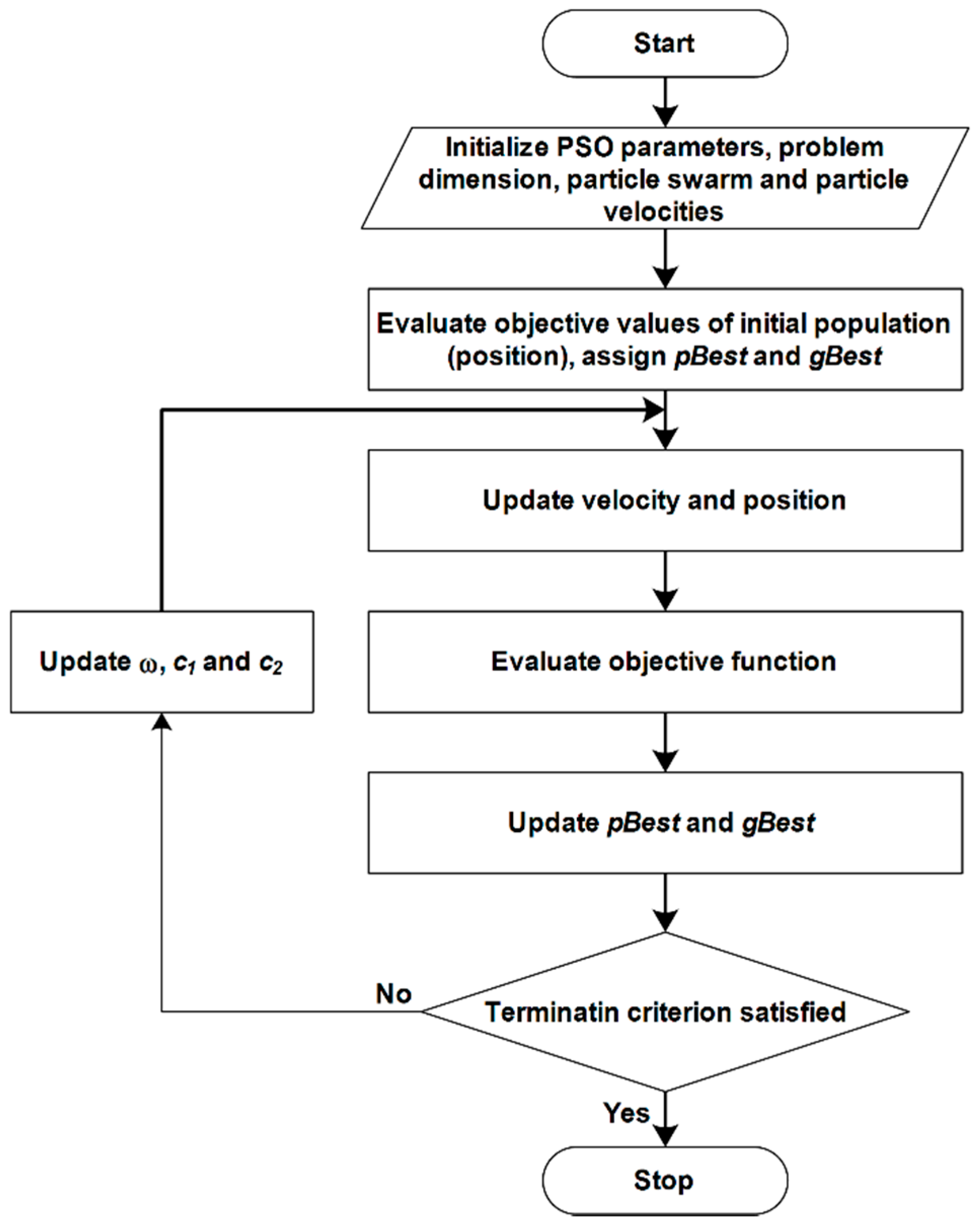
For obtaining coefficients for the two models, separate iterative routines were developed using the TVPSO optimization algorithm in MATLAB. The optimization algorithm requires a number of initial parameter settings. These settings are carefully selected so as to obtain convergence with the desired accuracy. Table 5 shows the parameter settings used in TVPSO, whereas Figure 3 shows the flow diagram of the TVPSO.

4. Formation of Regression Equations Using TVPSO Algorithm

Coefficients were obtained for both models using routines described in the previous section. These were subsequently used for the formulation of regression equations for resonant frequency and Q-factor. The algorithm utilized the values of the parameters mentioned in Table 3. However, data were utilized material wise for which the table was sorted accordingly. Regression equations were obtained which are presented model wise for different shield materials

4.1. Model-1

Non-interactive regression equations for resonant frequency and Q-factor were formulated using the coefficients, which were generated by the iterative routine for Model-1. These equations describe dependencies of these parameters over geometrical dimensions of the shield. Regression equations for resonant frequency and Q-factor pertaining to SRRs of different shield materials were obtained. The generalized forms of equations for resonant frequency and Q-factor are given in Equations (5) and (7), respectively. Coefficients for the two equations pertaining to Model-1 are given in Table 6 and Table 7, respectively.

4.2. Model-2

Interactive regression equations for resonant frequency and Q-factor were formulated in a similar manner. Coefficients were generated by the iterative routine for Model-2. These equations describe not only the dependencies of these parameters over geometrical dimensions of the shield but also the effect due to their interactions. Regression equations for resonant frequency and Q-factor pertaining to SRRs of different shield materials were obtained. Generalized forms of equations for resonant frequency and Q-factor are given in Equations (6) and (8), respectively. Coefficients for the two equations pertaining to Model-1 are given in Table 8 and Table 9, respectively.

5. Results and Discussion

Results for resonant frequency and Q-factor were obtained using both models. These were compared with the values obtained through HFSS simulations. Material wise coefficients and MAE pertaining to these parameters for Model-1 are tabulated in Table 6 and Table 7, whereas Table 8 and Table 9 present information for Model-2.
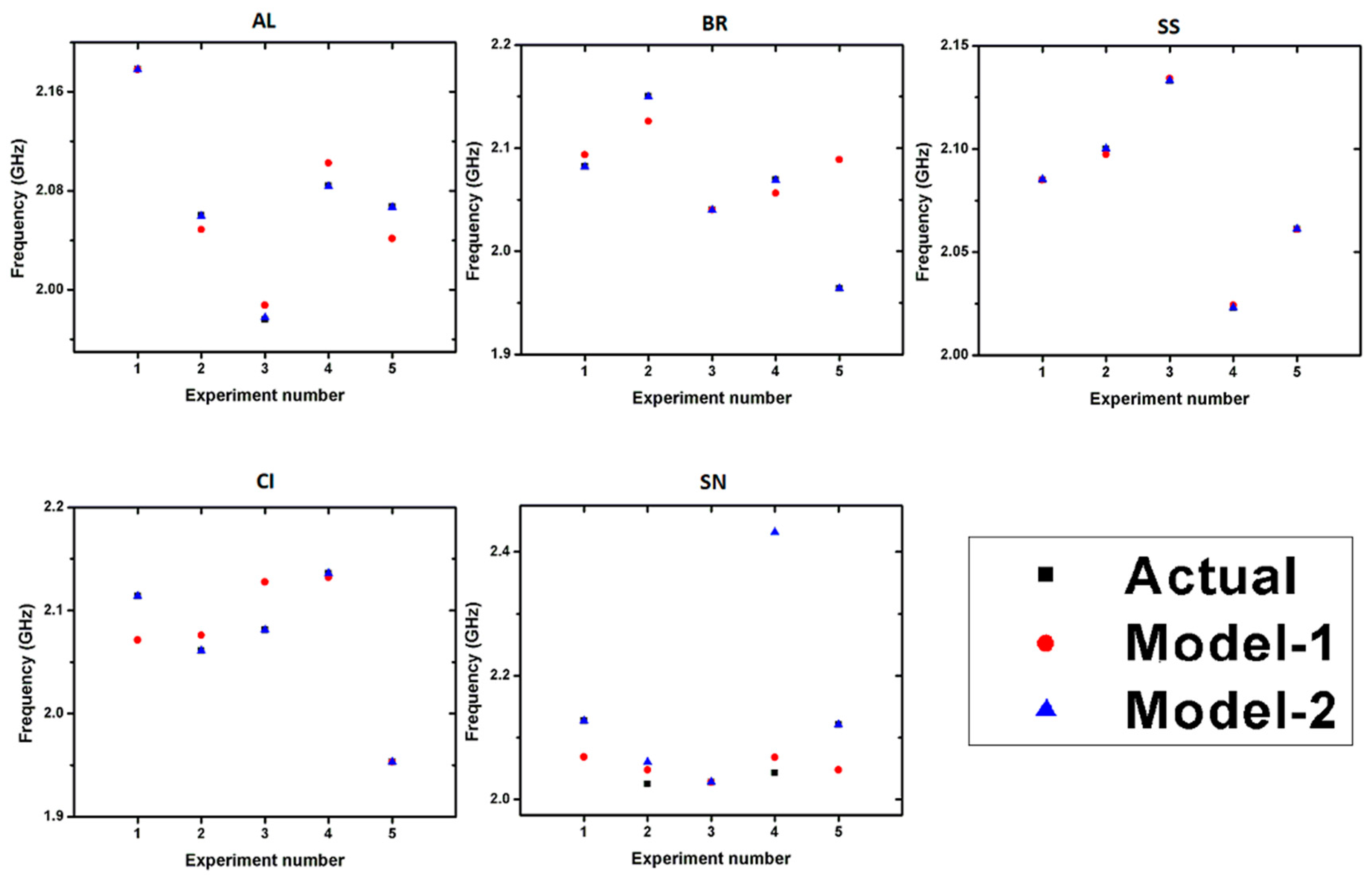
Table 10 tabulates the actual and estimated resonant frequency values along with the absolute error values. In Table 10, f a c t . represents the actual frequency values obtained through simulation whereas f 1 and f 2 represent the estimated frequency values by Model-1 and Model-2, respectively. These are also shown graphically in Figure 4. The difference between f a c t . and f 1 is represented by e 1 , and the difference between f a c t . and f 2 is represented by e 2 
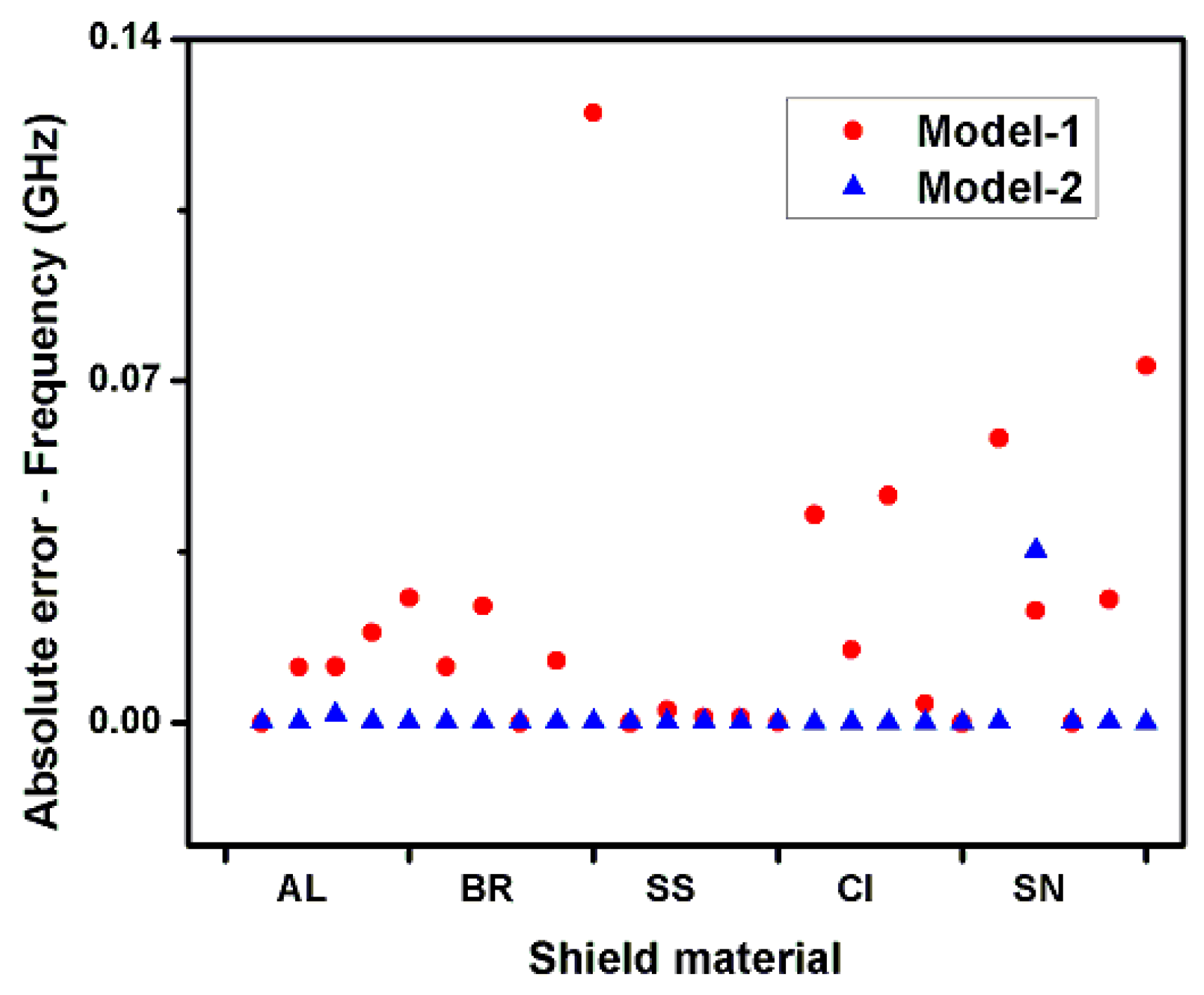
. Absolute error for frequency is shown graphically in Figure 5. On the whole, it is obvious from this table that the absolute values of e 2 are much less or nearly zero compared to the absolute values of e 1 . However, in some cells the absolute value of e 1 is better than the absolute value of e 2 . In overall comparison, Model-2 outperformed Model-1 in terms of achieving resonant frequency values overlapping actual values.
In a similar manner, the actual and estimated Q-factor values along with the absolute error values have been tabulated in Table 11. In this table, Q a c t . represents the actual Q-factor values obtained through simulation whereas Q 1 and Q 2 represent the estimated values by Model-1 and Model-2, respectively. These are also shown graphically in Figure 6. The difference between Q a c t . and Q 1 is represented by e 3 , and the difference between Q a c t . and Q 2 is represented by e 4 
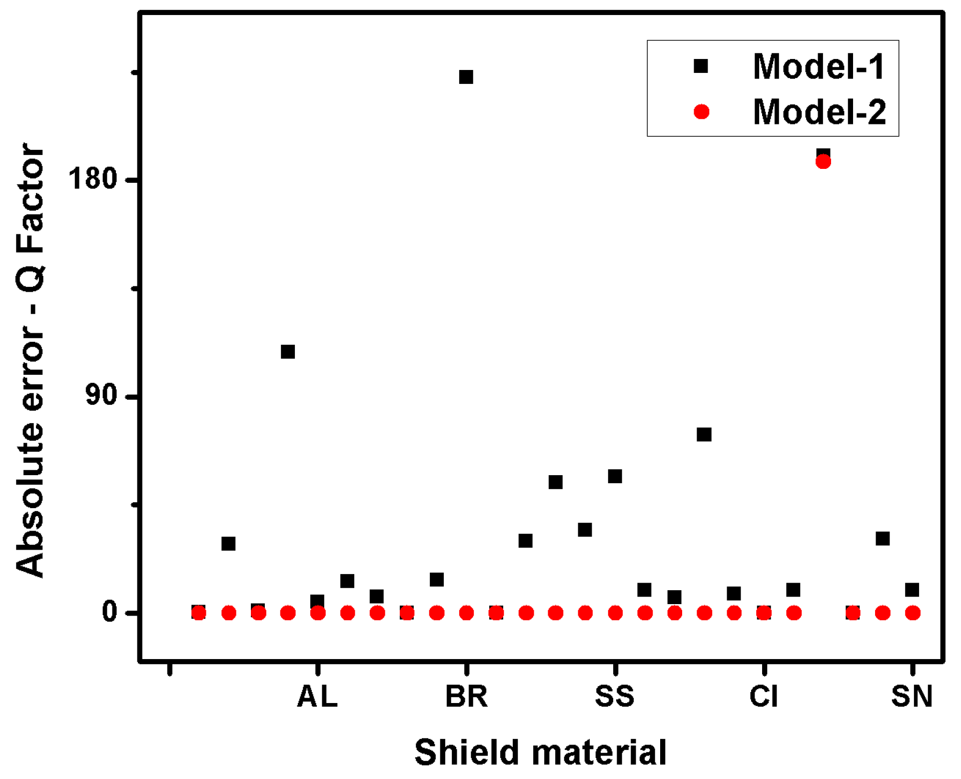
. The absolute error for frequency is shown graphically in Figure 7. On the whole, it is obvious from this table that the absolute values of e 4 are much less or nearly zero compared to absolute values of e 3 . In one instance however, absolute value of e 3 is better than the absolute value of e 4 . In this comparison also, Model-2 outperformed Model-1 in terms of achieving desired values.
It is clear from the above comparisons that Model-2 generated highly precise values both for resonant frequency and Q-factor compared to Model-1. This is primarily because Model-2 has been obtained keeping in mind the interactions between the dimensional parameters of SRR shields, whereas Model-1 does not cater for this aspect. Keeping in view this observation, better results can be expected while considering higher order interactions.

6. Conclusions

Values of the resonant frequency and Q-factor pertaining to SRR with different shield materials were obtained using two multi-coefficient models. A variant of the PSO algorithm with time-varying inertia and acceleration coefficients was used to optimize the models’ coefficients. Having the algorithm parameters as time-varying contributes towards good exploration and exploitation capabilities in order to avoid becoming trapped in a local solution. Results obtained through these models were compared with each other. Overall, Model-2 contributed well towards achieving very low objective (MAE) values when compared with Model-1. Average absolute errors generated by Model-1 for resonant frequency and Q factor were less than 4 and 3 percent, respectively; while Model-2 yielded results with average absolute errors even less than 1 percent for both parameters. It can thus be concluded that the interactive models were able to generate the expected results with higher accuracy and show a good match between the actual and calculated resonant frequency and Q-factor.

Author Contributions

Data curation, M.A.M. and T.E.; Formal analysis, M.A.M. and T.E.; Methodology, M.A.M.; Software, M.A.M.; Writing—original draft, M.A.M. and T.E.; Writing—review & editing, A.A. and A.H.

Funding

This research received no external funding.

Conflicts of Interest

The authors declare no conflict of interest.

References

  1. Rowe, D.J.; Abduljabar, A.A.; Porch, A.; Barrow, D.A.; Allender, C.J. Improved Split-Ring Resonator for Microfluidic Sensing. IEEE Trans. Microw. Theory Tech. 2014, 62, 1–11. [Google Scholar] [CrossRef]
  2. Faktorová, D. Complex Permittivity of Biological Materials Measurement at Microwave Frequencies. Meas. Sci. Rev. 2007, 7, 12–15. [Google Scholar]
  3. Eaton, S.S.; Eaton, G.R.; Berliner, L. Biological Magnetic Resonance: Biomedical EPR, Part B: Methodology, Instrumentation, and Dynamics, 1st ed.; Springer: New York, NY, USA, 2005; ISBN 978-0-306-48533-6. [Google Scholar]
  4. Venkatesh, M.S. Cavity Perturbation Technique for Measurement of Dielectric Properties of Some Agrifood Materials; McGill University: Montreal, QC, Canada, 1996. [Google Scholar]
  5. Galindo-romera, G.; Herraiz-martínez, F.J.; Gil, M.; Juan, J.; Segovia-vargas, D. Submersible Printed Split-Ring Resonator-Based Sensor for Thin-Film Detection and Permittivity Characterization. IEEE Sens. J. 2016. [Google Scholar] [CrossRef]
  6. Masood, A. Microwave Resonator for Highly Sensitive Compositional Analysis of Solvents in Mictocapillary Systems; Cardiff University: Cardiff, UK, 2009. [Google Scholar]
  7. Venkatesh, M.S.; Raghavan, G.S.V. An overview of microwave processing and dielectric properties of agri-food materials. Biosyst. Eng. 2004, 88, 1–18. [Google Scholar] [CrossRef]
  8. Gwinner, M.C.; Koroknay, E.; Liwei, F.; Patoka, P.; Kandulski, W.; Giersig, M.; Giessen, H. Periodic large-area metallic split-ring resonator metamaterial fabrication based on shadow nanosphere lithography. Small 2009, 5, 400–406. [Google Scholar] [CrossRef] [PubMed]
  9. Ejaz, T.; Ur Rahman, H.; Tauqeer, T.; Masood, A.; Zaidi, T. Shield Optimization and Formulation of Regression Equations for Split-Ring Resonator. Math. Probl. Eng. 2016, 2016, 4754192. [Google Scholar] [CrossRef]
  10. Hardy, W.N.; Whitehead, L.A. Split-ring resonator for use in magnetic resonance from 200–2000 MHz. Rev. Sci. Instrum. 1981, 52, 213–216. [Google Scholar] [CrossRef]
  11. Froncisz, W.; Hyde, J.S. The loop-gap resonator: A new microwave lumped circuit ESR sample structure. J. Magn. Reson. 1982, 47, 515–521. [Google Scholar] [CrossRef]
  12. Hyde, J.S. Multipurpose Loop-Gap Resonator. J. Magn. Reson. 1989, 230, 223–230. [Google Scholar] [CrossRef]
  13. Ejaz, T.; Rahman, H.U.; Afaq, S.; Shah, A.; Zaidi, T. A Comparative Analysis of Split-Ring Resonator Models. In Proceedings of the 4th International Conference on Informatics, Electronics & Vision (ICIEV), Fukuoka, Japan, 15–18 June 2015. [Google Scholar]
  14. Boccard, J.; Aftab, T.; Hoppe, J.; Yousaf, A.; Huetter, R.; Reindl, L.M.; Member, I.S. High-Resolution, Far-field and Passive Temperature Sensing up to 700 °C using an Isolated ZST Microwave Dielectric Resonator. IEEE Sens. J. 2015, X, 1–8. [Google Scholar] [CrossRef]
  15. Cheng, H.; Member, S.; Ren, X.; Ebadi, S.; Chen, Y.; An, L.; Gong, X.; Member, S. Wireless Passive Temperature Sensors Using Integrated Cylindrical Resonator/Antenna for Harsh-Environment Applications. IEEE J. Photovolt. 2015, 15, 1453–1462. [Google Scholar] [CrossRef]
  16. Ejaz, T. Optimization of Spit-Ring and Split-Ball Resonators for Effective Permittivity and Volume Fraction Extraction; National University of Science & Technology: Islamabad, Pakistan, 2017. [Google Scholar]
  17. Chen, L.F.; Ong, C.K.; Neo, C.P.; Varadan, V.V.; Varadan, V.K. Microwave Electronics: Measurement and Materials Characterization; Wiley: Chichester, UK, 2004. [Google Scholar]
  18. Sydoruk, O.; Tatartschuk, E.; Shamonina, E.; Solymar, L. Analytical formulation for the resonant frequency of split rings. J. Appl. Phys. 2009, 105, 1–5. [Google Scholar] [CrossRef]
  19. Mehdizadeh, M.; Ishii, T.K.; Hyde, J.S.; Froncisz, W. Loop-Gap Resonator: A Lumped Mode Microwave Resonant Structure. IEEE Trans. Microw. Theory Tech. 1983, 31, 1059–1064. [Google Scholar] [CrossRef]
  20. Birnbaum, G.; Franeau, J. Measurement of the Dielectric Constant and Loss of Solids and Liquids by a Cavity Perturbation Method. J. Appl. Phys. 1949, 817, 13–15. [Google Scholar] [CrossRef]
  21. Masood, A.; Castell, O.; Barrow, D.; Allender, C.; Porch, A. Split ring resonator technique for compositional analysis of solvents in microcapillary systems. In Proceedings of the Twelfth International Conference on Miniaturized Systems for Chemistry and Life Sciences, San Diego, CA, USA, 12–16 October 2008; pp. 1636–1638. [Google Scholar]
  22. Ejaz, T.; Rahman, H.U.; Zaidi, T.; Tauqeer, T.; Afaq, S.; Shah, A. Analysis, Simulation and Experimental Verification of Split Ring Resonator. Microw. Opt. Technol. Lett. 2015, 57, 2358–2363. [Google Scholar] [CrossRef]
  23. Ansoft ANSYS HFSS. Available online: https://www.ansys.com/products/electronics/ansys-hfss (accessed on 1 September 2018).
  24. Minitab Statistical Software. Available online: https://www.minitab.com/en-us/ (accessed on 10 September 2018).
  25. Mughal, M.A.; Ma, Q.; Xiao, C. Photovoltaic cell parameter estimation using hybrid particle swarm optimization and simulated annealing. Energies 2017, 10, 1213. [Google Scholar] [CrossRef]
  26. Mughal, M.A.; Khan, M.; Shah, A.A.; Almani, A. DC Motor Parameter Estimation Using Chaotic Initialized Particle Swarm Optimization. In Proceedings of the 3rd International Conference on Electromechanical Control and Transportation (ICECTT), Chongqing, China, 19–21 January 2018. [Google Scholar]
  27. Martins, S.; Ribeiro, C. Metaheuristics and applications to optimization problems in telecommunications. In Handbook of Optimization in Telecommunications; Springer: Boston, MA, USA, 2006; pp. 3–28. [Google Scholar]
  28. Karaboga, N. Digital IIR Filter Design Using Differential Evolution Algorithm. EURASIP J. Adv. Signal Process. 2005, 2005, 1269–1276. [Google Scholar] [CrossRef]
  29. Jiang, S.; Wang, Y.; Ji, Z. A new design method for adaptive IIR system identification using hybrid particle swarm optimization and gravitational search algorithm. Nonlinear Dyn. 2015, 79, 2553–2576. [Google Scholar] [CrossRef]
  30. Chih, M.; Lin, C.; Chern, M.; Ou, T. Particle swarm optimization with time-varying acceleration coefficients for the multidimensional knapsack problem. Appl. Math. Model. 2014, 38, 1338–1350. [Google Scholar] [CrossRef]
  31. Mohammadi-ivatloo, B.; Rabiee, A.; Ehsan, M. Time-varying acceleration coefficients IPSO for solving dynamic economic dispatch with non-smooth cost function. Energy Convers. Manag. 2012, 56, 175–183. [Google Scholar] [CrossRef]
  32. Bluman, A.G. Elementary Statistics: A Step by Step Approach; Mcgraw Hill: New York, NY, USA, 2012; ISBN 978-0072549072. [Google Scholar]
  33. Proust, M. Design of Experiments Guide; SAS Institute: Cary, NC, USA, 2007; ISBN 9781599944135. [Google Scholar]
  34. Jordehi, A.R. Time varying acceleration coefficients particle swarm optimisation (TVACPSO): A new optimisation algorithm for estimating parameters of PV cells and modules. Energy Convers. Manag. 2016, 129, 262–274. [Google Scholar] [CrossRef]
  35. Shi, Y.; Eberhart, R. A modified particle swarm optimizer. In Proceedings of the 1998 IEEE International Conference on Evolutionary Computation Proceedings, IEEE World Congress on Computational Intelligence (Cat. No. 98TH8360), Anchorage, AK, USA, 4–9 May 1998; pp. 69–73. [Google Scholar] [CrossRef]
  36. Chaturvedi, K.T.; Pandit, M.; Srivastava, L. Particle swarm optimization with time varying acceleration coefficients for non-convex economic power dispatch. Int. J. Electr. Power Energy Syst. 2009, 31, 249–257. [Google Scholar] [CrossRef]
Figure 1. Split-ring resonator enclosed in cavity, front (L) and top (R) view.
Electronics 07 00300 g001
Figure 2. HFSS software simulation of a split-ring resonator (SRR).
Electronics 07 00300 g002
Figure 3. Flow diagram of the TVPSO.
Electronics 07 00300 g003
Figure 4. Estimated frequency values of Model-1 and Model-2.
Electronics 07 00300 g004
Figure 5. Absolute errors for frequency pertaining to shields of different materials.
Electronics 07 00300 g005
Figure 6. Estimated Q-factor values of Model-1 and Model-2.
Electronics 07 00300 g006
Figure 7. Absolute errors for Q-factor pertaining to shields of different materials.
Electronics 07 00300 g007
Table 1. Properties of shield material.
Shield MaterialRelative Permeability μ r Bulk Conductivity σ, SiemensMass Density ρ, kg/m3
AL1.00002138,000,0002689
BR115,000,0008600
SS11,100,0008055
CI601,500,0007200
SN18,670,0007304
Table 2. Parameters of base design SRR.
Design ParametersDimensions (mm)
Inner radius of shield “R025
Inner radius of resonator “r06
Width of resonator “W6
Length of resonator “Z6
Gap of resonator “t2
Inner height of shield “H28
Thickness of shield “T” (in all directions)4
Table 3. Range of parametric variations.
ParametersRange of Variation
Minimum (mm)Maximum (mm)Increment (mm)
Inner height of shield “H28321
Inner radius of shield “R025291
Thickness of shield “T” (in all directions)481
Table 4. L-25 array with values of resonant frequency and Q-factor.
Height of Shield (mm)Radius of Shield (mm)Thickness of Shield (mm)Shield MaterialResonant Frequency (GHz)Q-Factor
28254AL2.1783147.49
28265BR2.0822750.86
28276SS2.0852399.01
28287CI2.1141217.51
28298SN2.1272785.92
29255SS2.1002465.01
29266CI2.0611234.29
29277SN2.0252596.40
29288AL2.0602895.21
29294BR2.1502607.00
30256SN2.0282796.62
30267AL1.9762573.34
30278BR2.0402619.77
30284SS2.1332542.19
30295CI2.0811352.58
31257BR2.0692728.93
31268SS2.0232419.74
31274CI2.1361271.32
31285SN2.0432775.66
31296AL2.0842962.62
32258CI1.9531251.17
32264SN2.1212826.00
32275AL2.0672763.36
32286BR1.9642328.57
32297SS2.0612321.32
Table 5. TVPSO parameters.
ParametersSetting
Swarm size5000
Number of iterations100
ω (0.4, 0.9)
c 1 (0.5, 2.5)
c 2 (0.5, 2.5)
Table 6. Optimized coefficients for resonant frequency using Model-1.
MaterialCoefficientsMAE
a 0 a 1 a 2 a 3
AL2.6004−0.03950.0352−0.0489 1.3 × 10 2
BR2.04610.00230.0033−0.0205 3.46 × 10 2
SS2.1658−0.00230.0049−0.0245 1 × 10 3
CI2.4399−0.01340.0094−0.0367 2.16 × 10 2
SN−1.20080.08190.01210.0780 3.6 × 10 2
Table 7. Optimized coefficients for Q-factor using Model-1.
MaterialCoefficientsMAE
b 0 b 1 b 2 b 3
AL3630.23−140.1566161.9139−151.558324.522
BR4844.7288−23.4483−51.8445−15.213551.3
SS2773.114.9930−20.5774−39.710935.12
CI569.000514.96709.9874−5.807619.608
SN2093.00721.2604−0.081611.306647.972
Table 8. Optimized coefficients for resonant frequency using Model-2.
MaterialCoefficientsMAE
a 0 a 1 a 2 a 3 a 4 a 5 a 6
AL−0.6931−0.0275−0.00851.47270.0054−0.0348−0.0193 7.1468 × 10 12
BR0.08810.05030.4575−1.6877−0.01490.0565 3.5958 × 10 4 2.2723 × 10 12
SS4.0439−0.03641.0166−4.9398−0.03460.15150.0119 2.4821 × 10 11
CI1.1301−0.1801−0.48723.26910.0237−0.0733−0.0380 4.9702 × 10 11
SN1.20120.02241.90631.0571−0.0518−0.0336−0.0599 7.0194 × 10 3
Table 9. Optimized coefficients for resonant Q-factor using Model-2.
MaterialCoefficientsMAE
b 0 b 1 b 2 b 3 b 4 b 5 b 6
AL4303.33−85.98−36.41452.043.73−27.388.09 8.6953 × 10 9
BR2873.80−145.95134.25718.730.339.15−35.72 1.57 × 10 9
SS493.70−30.2578.23529.301.241.73−23.26 1.5623 × 10 9
CI1608.40−189.14−33.95914.697.77−3.84−30.03 6.1021 × 10 9
SN1902.7035.53582.76342.75−16.20−10.80−18.0037.5346
Table 10. Comparison of actual and estimated resonant frequency using Model-1 and Model-2.
Material f a c t . ( GHz ) Model-1Model-2
f 1   ( GHz ) a b s   ( e 1 ) f 2   ( GHz ) a b s   ( e 2 )
AL2.1782.17802.17780.0002
2.062.04860.01142.05970.0003
1.9761.98750.01151.97770.0017
2.0842.10250.01852.08370.0003
2.0672.04140.02562.06680.0002
BR2.0822.09350.01152.08180.0002
2.152.12610.02392.14980.0002
2.042.0402.03970.0003
2.0692.05630.01272.06870.0003
1.9642.08880.12481.96380.0002
SS2.0852.08502.08520.0002
2.12.09740.00262.10020.0002
2.1332.13420.00122.13320.0002
2.0232.02420.00122.02320.0002
2.0612.06090.00012.06130.0003
CI2.1142.07140.04262.11400
2.0612.0760.0152.06100
2.0812.12750.04652.08090.0001
2.1362.1320.0042.13590.0001
1.9531.95301.9530
SN2.1272.06880.05822.12720.0002
2.0252.0480.0232.06030.0353
2.0282.02802.02820.0002
2.0432.06830.02532.04320.0002
2.1212.04790.07312.12110.0001
Table 11. Comparison of actual and estimated Q-factor using Model-1 and Model-2.
Material Q a c t . Model-1Model-2
Q 1 a b s   ( e 3 ) Q 2 a b s   ( e 4 )
AL3147.493147.230.263147.48990.0001
2895.212866.559928.65012895.21000
2573.342574.13990.79992573.34000
2962.623071.27108.652962.62000
2763.362758.84994.51012763.35990.0001
BR2750.862764.12113.2612750.87470.0147
26072600.3156.6852607.01690.0169
2619.772619.7410.0292619.78290.0129
2728.932715.19613.7342728.94530.0153
2328.572551.426222.8562328.58860.0186
SS2399.012399.0590.0492399.03110.0211
2465.012494.91729.9072465.0310.021
2542.192487.8954.32542.2140.024
2419.742385.19334.5472419.7650.025
2321.322378.16656.8462321.3480.028
CI1217.511227.079.561217.570.06
1234.291227.86986.42021234.330.04
1352.581278.606673.97341352.620.04
1271.321279.40648.08641271.3470.027
1251.171251.16820.00181251.2260.056
SN2785.922776.38599.53412785.920
2596.42786.5029190.1032784.0729187.6729
2796.622796.6202796.620
2775.662806.328930.66892775.660
28262816.4469.55428260

