Free-Space Materials Characterization by Reflection and Transmission Measurements using Frequency-by-Frequency and Multi-Frequency Algorithms

Abstract

The knowledge of the electromagnetic constitutive properties of materials is crucial in many applications. Free-space methods are widely used for this purpose, despite their inherent practical difficulties. This paper describes an affordable free-space experimental setup for the characterization of flat samples in 1–6 GHz in a non-anechoic environment. The extracted properties are obtained from the calibrated Scattering Parameters, using a frequency-by-frequency solution or a multi-frequency reconstruction. For the first, we describe how the Time-Domain Gating can be implemented and used for filtering the signals. For the latter, a weighting factor is introduced to balance the reflection and transmission data, allowing one to have a more favorable configuration. The different role of transmission and reflection measurements on the achievable results is analyzed with regard to experimental uncertainties and different noise scenarios. Results from the two strategies are analyzed and compared. Good agreement between simulation, measurement and literature is obtained. According to the reported results for dielectric materials, there is no need of filtering the data by a Time-Domain Gating in case of the multi-frequency approach. Experimental results for Polymethylmethacrylate (PMMA) and Polytetrafluorethylene (PTFE) samples validate both the setup and the processing.

1. Introduction

Characterization of the electric permittivity $\epsilon$, the magnetic permeability $\mu$ and the electric conductivity $\sigma$ is of fundamental importance in physics and engineering, since these constitutive properties determine the response of the Material Under Test (MUT) to the electromagnetic fields [1,2]. Usually, such properties are extracted from the Scattering (S-) Parameters [1,2,3,4], which can be measured by a Vector Network Analyzer (VNA) [3]. Several measurement setups can be conceived for this purpose, including the Free-Space Method (FSM) [1].

The FSM consists in connecting antennas to the ports of a VNA and using them to sense the propagation path of interest; in this way, different materials can be characterized by means of proper reconstruction algorithms [1,3,4,5,6]. The FSM is contactless, requires little sample preparation and is suitable for heterogeneous samples. It can be used for measuring large flat solids, materials under high temperature [7], liquids [8], gases [1,6], radomes in aerospace [9], multi-layered dielectrics [10], composite materials and metamaterials [11,12,13,14]. One should note that the effective response, the non-invasive nature and the wideband operation are essential in many actual applications.

The FSM is commonly used to characterize building materials in order to estimate their influence on telecommunications [15,16,17] or in through-wall imaging [18]. Moreover, the knowledge of the electromagnetic properties can be used to evaluate the physical conditions of materials in different areas, such as masonry structures in civil engineering [17,19,20], the characteristics of snow [21] or even agricultural materials [22]. There are also several works in millimeter wavelengths, for instance, for characterizing dielectrics [23], electromagnetic absorbers [24] and nanocomposites [25].

The concept of transmission and reflection FSM is shown in Figure 1. Antennas and the space therein can be considered as a two port network whose behavior is characterized by its four S-Parameters: $S_{11}$, $S_{12}$, $S_{21}$ and $S_{22}$ [3,26]. After the measurement, the S-Parameters are used for extracting the electromagnetic properties of the sample. However, the measured S-Parameters are influenced by multipath propagation, unwanted reflections and other interferences, especially in a non-anechoic environment. As a consequence, additional signal processing is often required.

Two techniques are important to deal with the above mentioned free-space configuration: (a) the free-space calibration [1,14,27], intended to normalize the measurements and to dislocate the calibration planes to the surfaces of the sample; and (b) the Time-Domain Gating (TDG) [1,3,26,27,28,29,30,31], intended to filter the measured signals. After such preprocessing, the resulting signal can be used to recover the material properties by different extraction techniques.

In this paper two recovery approaches are presented and analyzed, using simulated and experimental data. One approach assumes to deal with non dispersive materials and its multi-frequency solution is based on the minimization of a properly defined functional. The other is a frequency-by-frequency approach, in which a possible dispersion in the measurement range is assumed, without a previous knowledge of the dispersion model of the material. Both the approaches rely on the same one dimensional model of scattering, where the measured S-Parameters are interpreted as the reflection and transmission coefficient of an equivalent transmission line.

In particular, some contributions of this work are: (a) a weighted and normalized cost function is introduced for the multi-frequency extraction from $S_{11}$ and $S_{21}$; it is studied in terms of signal to noise levels, different weights for transmission/reflection and it is applied to free-space measurements; (b) an affordable experimental setup is presented and its calibration is discussed; (c) an analysis of uncertainty is presented; (d) the implemented TDG is explained and its applicability to the extraction methods is discussed.

The paper is organized as follows. In Section 2 we present the mathematical model, the extraction algorithms, the experimental setup and its calibration and, at last, the signal processing. The effect of the measurement uncertainties is analyzed in Section 3. Afterwards, numerical and experimental results are presented and discussed in Section 4. The conclusions are in Section 5.

2. Materials and Methods

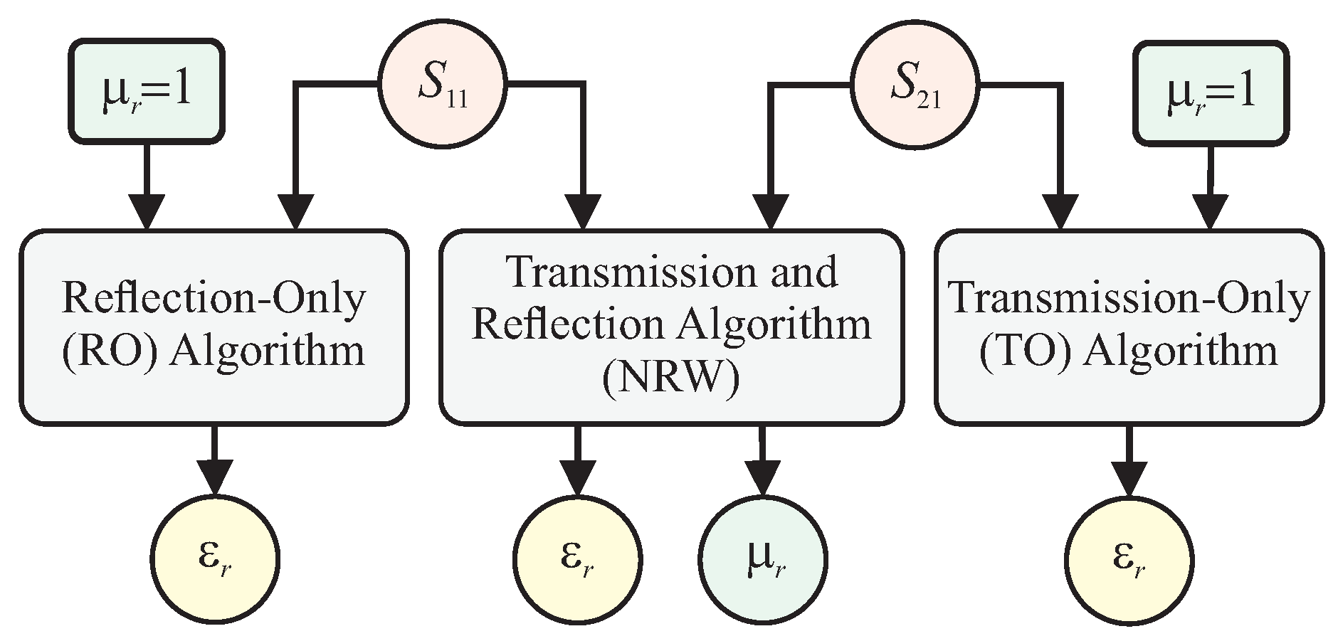
2.1. Slab Scattering Model

The relationship between the scattered field and the electromagnetic properties of the material under test is provided by assuming an one dimensional geometry, where an incident plane wave is reflected (by) and transmitted (through) a planar homogeneous slab of relative electric permittivity ${\epsilon }_r$, relative magnetic permeability ${\mu }_r$ and electric conductivity $\sigma$. This allows to apply the equivalent transmission line equations for time harmonic fields at the frequency f [2].

In this way, the reflection coefficient, defined as the ratio between the reflected and the incident field at the first slab interface, can be expressed as the following function of the slab properties:

$$F_R({\epsilon }_r,{\mu }_r,\sigma )=\frac{j(y^2-1)\tau }{2y+j(y^2+1)\tau },$$

(1)

where the auxiliary variables $y=\sqrt{{\mu }_r/({\epsilon }_r-j\sigma /\omega {\epsilon }_0)}$, $\tau =tan(\omega xd/c)$ and $x=\sqrt{{\mu }_r({\epsilon }_r-j\sigma /\omega {\epsilon }_0)}$ are introduced; d is the thickness of the sample, j is the imaginary unit, $\omega =2\pi f$ is the angular frequency; c and ${\epsilon }_0$ are the free space electromagnetic wave speed and dielectric permittivity, respectively. Note that y and $1/x$ are the impedance and wave speed of the material, normalized to free space, respectively.

In its turn, the transmission coefficient, defined as the ratio between the transmitted field at the second slab interface and the incident field at the first slab interface, can be expressed as:

$$F_T({\epsilon }_r,{\mu }_r,\sigma )=\frac{2y}{cos(\omega xd/c)[2y+j(y^2+1)\tau ]}.$$

(2)

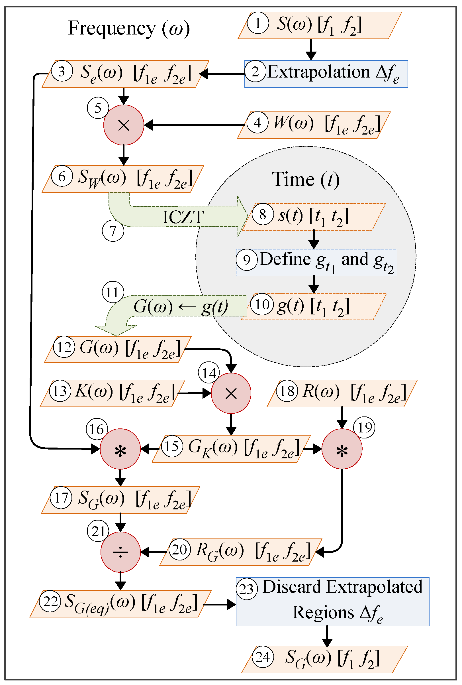
2.2. Multi-Frequency Extraction

When the MUT is non dispersive in the investigated frequency band, a possible strategy in order to estimate the unknown material properties from the reflection and transmission coefficients is to minimize the “distance” between theoretical and measured quantities. Optimization-based reduction is interesting because correlations between frequency measurements are allowed [32]. It can be done by searching for the global minimum of a normalized cost function, here defined as:

$$\mathsf{\Psi }({ϵ}_r,{\mu }_r,\sigma )=w\frac{\left|\right|F_R-S_{11}{\left|\right|}^2}{\left|\right|S_{11}{\left|\right|}^2}+(1-w)\frac{\left|\right|F_T-S_{21}{\left|\right|}^2}{\left|\right|S_{21}{\left|\right|}^2},$$

(3)

where $\left|\right|·{\left|\right|}^2$ is the quadratic norm. The scattering parameters $S_{11}$ and $S_{21}$ play the role of data of the problem, that can be either measured by the VNA or numerically simulated. The value of the weighting coefficient w can be fixed in the interval $0\le w\le 1$, in order to enhance the role of either the reflection or the transmission.

The non linear nature of the relationships (1) and (2) makes the functional (3) non-quadratic, so that local minima can occur. Moreover, ill conditioning may affect the minimization procedure when reflection and transmission weakly depend on the material properties. In this case, a proper tuning of w can help in improving the functional behavior.

If the MUT is dispersive but its properties obey a dispersion model, the Debye or Lorentz for example, it can be included in the procedure and its characteristic parameters must be calculated [1,4]. Otherwise, a frequency-by-frequency approach can be used, but this one does not exploit the multi-frequency nature of the measurement, as explained next.

2.3. Frequency-by-Frequency Extraction

Here, the complex scattering parameters $S_{11}$ and $S_{21}$ are input data to three extraction algorithms, as illustrated in Figure 2 and explained afterwards: (a) the Nicolson-Ross-Weir (NRW) Algorithm, (b) The Reflection-Only (RO) Algorithm, and (c) The Transmission-Only (TO) Algorithm. These are frequency-by-frequency methods, since the properties are extracted for each particular frequency [1], in a point-to-point sweep. In the following the relative permittivity and permeability are assumed to be complex, that is, ${\epsilon }_r={\epsilon }_r^{\prime }-j{\epsilon }_r^{″}$ and ${\mu }_r={\mu }_r^{\prime }-j{\mu }_r^{″}$, respectively.

The NRW [33,34] is the most traditional algorithm for retrieving ${\epsilon }_r$ and ${\mu }_r$ from $S_{11}$ and $S_{21}$. In a transmission line, these parameters are defined as in (4) and (5), where $\mathsf{\Gamma }$ and T are the interfacial reflection and the propagation coefficients, respectively. Because it is a well-established algorithm, its development is left to Appendix A.

$$S_{11}={\displaystyle \frac{(1-T^2)\mathsf{\Gamma }}{1-T^2{\mathsf{\Gamma }}^2}}.$$

(4)

$$S_{21}={\displaystyle \frac{(1-{\mathsf{\Gamma }}^2)T}{1-T^2{\mathsf{\Gamma }}^2}}.$$

(5)

However, when using NRW the results diverge for low loss materials in multiple integers of half wavelength in the sample. At these frequencies $|S_{11}|$ is too small and the equations become algebraic unstable as $|S_{11}|\to 0$. Moreover, the uncertainty in the measured phase is high for small $|S_{11}|$ [1,6,35,36]. In contrast, when the sample is thick and lossy, $S_{21}$ is small and its measurement can present a low Signal-to-Noise Ratio (SNR).

Alternative algorithms were also developed, exploiting only reflection or only transmission measurements [1,6,35,36]. However, in this case only one between ${\epsilon }_r$ and ${\mu }_r$ can be determined, due to the reduced available information. Because ordinary materials are usually non-magnetic in microwave frequencies, ${\mu }_r=$ 1 is often assumed and ${\epsilon }_r$ is calculated by finding the root of a function $F\left({\epsilon }_r\right)$, as described next.

The Reflection-Only (RO) method is particularly interesting when $S_{21}$ is unavailable or unreliable. In this case only $S_{11}$ is used. In order to have the function $F_{RO}$ in (6), one should consider ${\mu }_r=1$ in (1) and calculate the difference between the datum $S_{11}$ and the function $F_R$. The solution is found by forcing it to zero:

$$F_{RO}\left({\epsilon }_r\right)\equiv S_{11}+{\displaystyle \frac{({\epsilon }_r-1)tan\left(\nu \right)}{2\sqrt{{\epsilon }_r}+j({\epsilon }_r+1)tan\left(\nu \right)}}=0,$$

(6)

where $\nu =d(\omega /c)\sqrt{{\epsilon }_r}$.

The Transmission-Only (TO) method uses only $S_{21}$ and it is more interesting when $S_{11}$ is more susceptible to errors. The function $F_{TO}$ in (7) is obtained by considering ${\mu }_r=1$ in (2) and comparing the datum $S_{21}$ and the function $F_T$. Again, after some rearrangements the solution of the problem is the value of ${\epsilon }_r$ that satisfies the equation:

$$F_{TO}({\epsilon }_r)\equiv S_{21}\left[{\epsilon }_r\cos \left(\nu \right)+j\sqrt{\frac{{\epsilon }_r}{4}}(1+{\epsilon }_r)\sin \left(\nu \right)\right]-{\epsilon }_r=0.$$

(7)

One could use also the noniterative method in [36] to overcome the instabilities of NRW; it is restricted, however, for low-loss non-magnetic materials.

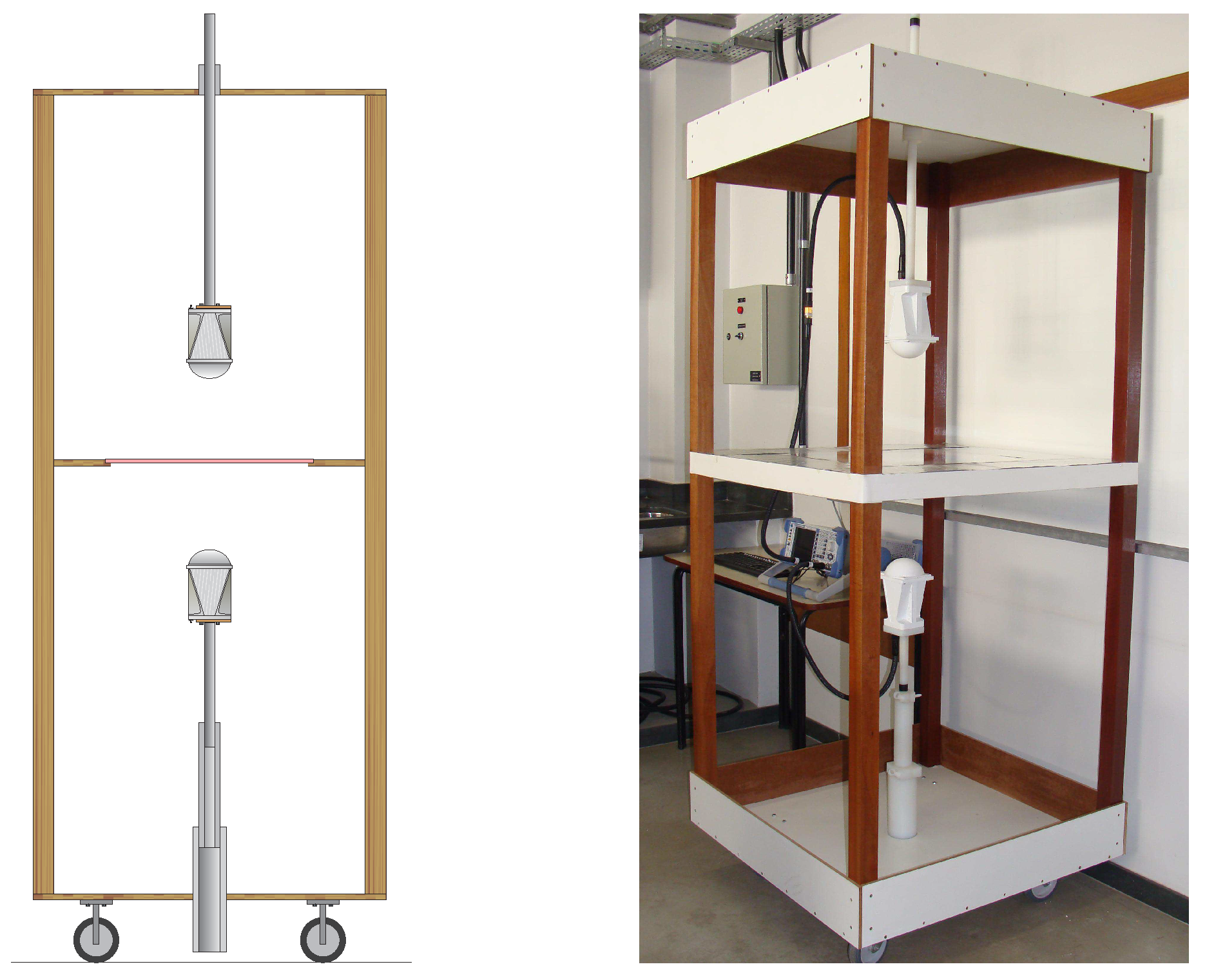
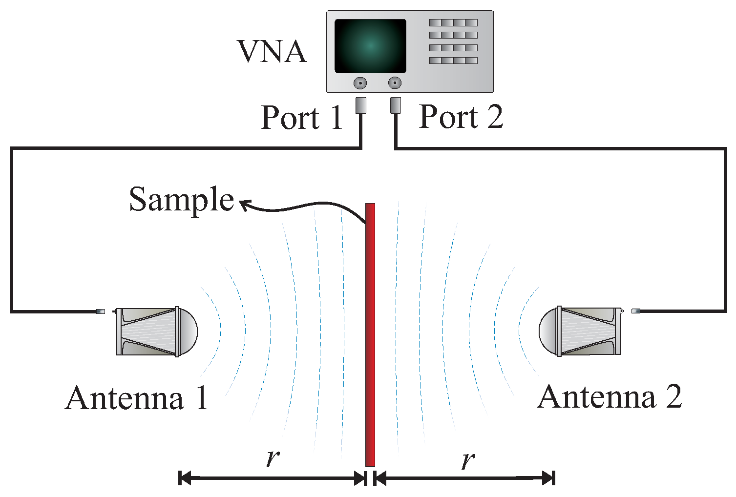
2.4. Experimental Setup

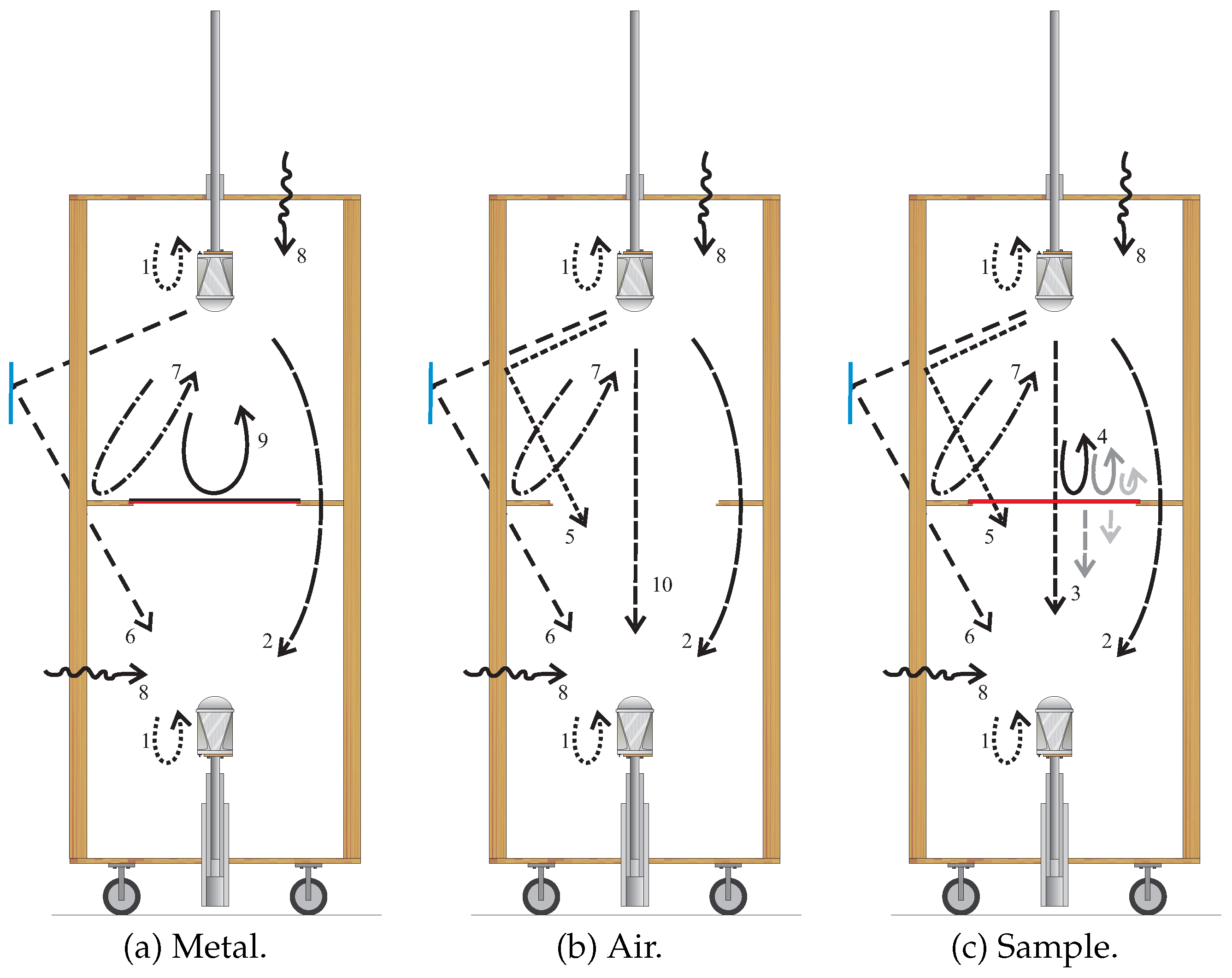
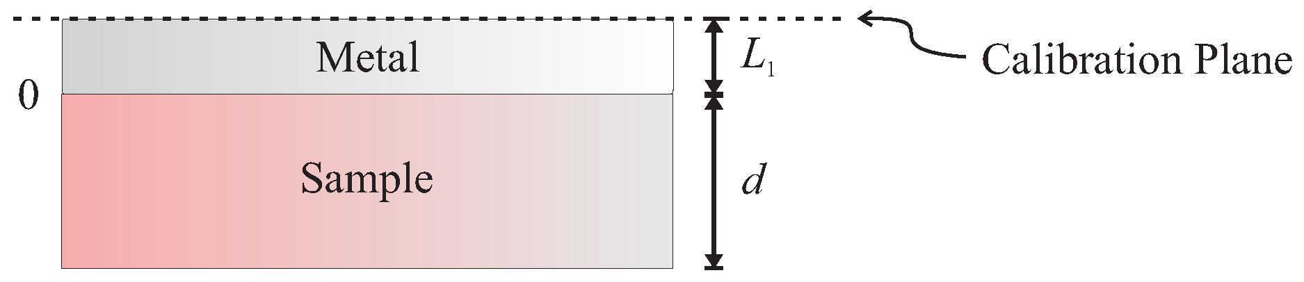
The experimental setup is at the Laboratory of Applied Electromagnetics of the Federal University of Minas Gerais. In order to reduce the reflections on the structure, metallic materials are avoided. So, as can be seen in Figure 3, the structure is made with wood and plywood. Each antenna is attached to a custom-made plastic telescoping stand. Aiming simplicity and low cost, the setup does not include electromagnetic absorbers.

The measurement setup has 2.1 × 0.85 × 0.85 m (height, width, depth). The sample holder is a squared frame with 0.5 m edges and the sample is supported by a 0.5 cm border around the squared hole in the middle of the setup. Because of that, the sample should be quite rigid. Alternatively, a rigid block of styrofoam can be used to support smaller samples or samples that bend.

We use two broadband horns with dielectric lenses (model Q-Par WBH1-18S14L). The lenses help to concentrate more radiation on the sample. The test range is 1–6 GHz, limited by the antennas (1–18 GHz) and by the VNA (9 kHz–6 GHz).

It is crucial that most of the electromagnetic energy passes through the sample. Thus, the dimensions of the setup are defined in a way that the half-power beamwidth (HPBW) [37] is entirely on the sample for the frequencies in our range.

On the actual configuration, the distance r between the antennas and the sample can vary between 0.3 m and 0.48 m. Furthermore, the design also permits that the main part of the radiation reaches the sample with similar phases, that is, the far-field condition [37]. Thus, r satisfies (8), where D is the largest aperture of the antenna and $\lambda$ is the wavelength [1,37]. Satisfying (8), the free-space can be approximated as an uniform transmission line [1]. In our case, the last condition in (8) is barely satisfied with $r=$ 0.3 m when D is large compared to $\lambda$ (above 2 GHz, approximately).

$$r>\lambda ,\hspace{1em}r>D,\hspace{1em}r>(2D^2)/\lambda .$$

(8)

2.5. Calibration

Two physical calibrations are performed in order to obtain the scattering coefficients of the MUT: (a) the VNA calibration, and (b) the free-space calibration. The first one is the Full 2-Port Calibration, in which the standards Through, Open, Short and Match (TOSM) of the Calibration Kit are used to compensate the effects of the cables [3,26]. Thus, the reference planes are shifted to the antennas connectors. The second one is the free-space calibration, where two reference measurements are performed, one in absence of the sample and the other in presence of a metallic plate. The aim is to remove undesired contributions and to move the calibration plane to the faces of the sample [27,38].

Each calibrated scattering parameter is obtained by three measurements: (a) measuring a metal plate with the same cross section of the sample; (b) leaving the setup empty; and, finally, (c) measuring the material under test (sample) [27,38]. Figure 4 illustrates possible contributions to the measured signals: reflections at the antennas due to mismatches (arrow 1); diffracted signal (arrow 2); signal transmitted through the sample and its secondary components (arrow 3); multiple reflections on the sample (arrow 4); signal reflected somewhere and passed through the sample area (arrow 5); signal reflected somewhere but did not cross the sample area (arrow 6); signal reflected somewhere and returned to antenna 1 (arrow 7); external influences that are not systematic and must be treated as noise (arrow 8); signal reflected on the metallic plane (arrow 9); and the transmitted signal at the empty setup (arrow 10).

Observe that the arrows in Figure 4 can be interpreted as the error terms of the signal flow graphs (errors-adapters) in microwave networks [3,17,26].

It has to be stressed that the reversed path, with $S_{12}$ and $S_{22}$, is not used in this work in order to reduce the measurement complexity.

In particular, measurement with empty setup (air) $S_{11}^{\left(\mathrm{air}\right)}$ allows to evaluate the contributions indicated by the arrows 1 and 7. In this way, $S_{11}^{\left(\mathrm{air}\right)}$ should be subtracted to $S_{11}$ for calibration, as in (9). Then, MUT measurement is normalized with that in the presence of the metal plate (metal), whose ideal reflection coefficient is −1. In a dual way, the contributions indicated by the arrows 2 and 6 are evaluated by measurement with metal $S_{21}^{\left(\mathrm{metal}\right)}$. As in (10), it is subtracted for calibrating $S_{21}$ and we normalize it with the measurement in air, whose ideal transmission coefficient is 1 [17,38].

$$S_{11}^{(\mathrm{mut}\mathrm{calib}.)}=-{\displaystyle \frac{S_{11}^{\left(\mathrm{mut}\right)}-S_{11}^{\left(\mathrm{air}\right)}}{S_{11}^{\left(\mathrm{metal}\right)}-S_{11}^{\left(\mathrm{air}\right)}}}{e}^{2j(\omega /c)L_1}.$$

(9)

$$S_{21}^{(\mathrm{mut}\mathrm{calib}.)}={\displaystyle \frac{S_{21}^{\left(\mathrm{mut}\right)}-S_{21}^{\left(\mathrm{metal}\right)}}{S_{21}^{\left(\mathrm{air}\right)}-S_{21}^{\left(\mathrm{metal}\right)}}}{e}^{-j(\omega /c)d}.$$

(10)

The exponential terms in (9) and (10) adjust the phases, since we have to consider that the sample and the metal plate actually substitute a slab of air [15]. As illustrated in Figure 5, the correction is made using the thicknesses $L_1$ of the metal plate and d of the sample. In our experimental configuration, $L_1$ has a minor effect, since we use a very thin aluminum foil (0.01 mm). However, the effect could be not negligible in case one use a electrically thicker metal plate. In other words, it is important that the calibration planes have a considerable coincidence with the faces of the sample. This is challenging, since a different bending or deformity on the metallic plate with respect to the sample (or vice-versa), affect the phase, especially for higher frequencies.

Although there are different calibrations applicable to FSM, such as the Thru-Reflect-Line (TRL), Thru-Reflect-Match (TRM) [1,3] and the Gated-Reflect-Line (GRL) [39,40], the described free-space calibration is a post-processing procedure that does not involve movements of the antennas. Again, it is important to prevent movements on the setup, since small mispositionings can generate great errors when using free-space methods [1,27]. The classical TRL and TRM calibrations demand three reference standards. In particular, TRL demands an accurate positioning system to perform the Line standard. By its turn, TRM demands a well-matched absorber to perform the Match standard, which is a challenge for broadband measurements in free-space [40].

Similarly to the GRL, our calibration demands only the Thru (air) and Reflect (metal) standards. It is a two-tier procedure, since we firstly perform the TOSM to remove the effect of the cables. Note that the new GRL, that is, the GRL-1 (one-tier) described in [40] does not need the TOSM at the end of the cables. One should remember, however, that the measurement bandwidth and the number of points are limited, so a long network could result in a low Time-Domain (TD) resolution.

Because of the practical difficulties, thickness and position invariant calibrations has been investigated both in FD [41,42,43,44] and in TD [45]. Observe that the TD analysis has been used in the GRL calibration [39,40], for extracting a desired part of a network [46] and also in TD extraction from measured FD data [45]. In this way, it is interesting to have a flexible procedure for the signal processing.

Note that our extraction described in Section 2.2 differs from those introduced elsewhere [32,41,42,43,44] in a way we do not use the reverse path ($S_{12}$ and $S_{22}$), since it would demand the metal plate to be positioned also on the bottom face of the sample in order to perform the calibration. It would require an additional repositioning of the sample, which is, as explained, a source of errors.

We can assume that the systematic errors are removed by TOSM and free-space calibrations. The random errors, in their turn, are usually unpredictable and cannot be removed by the calibration [1]. However, the filtering property of the TDG can minimize part of them. Here we do not consider drift errors, since we assume that the working conditions do not change substantially from the calibration ones. In other words, measurements are performed no more than few minutes after the calibration and after the warming-up time of the VNA.

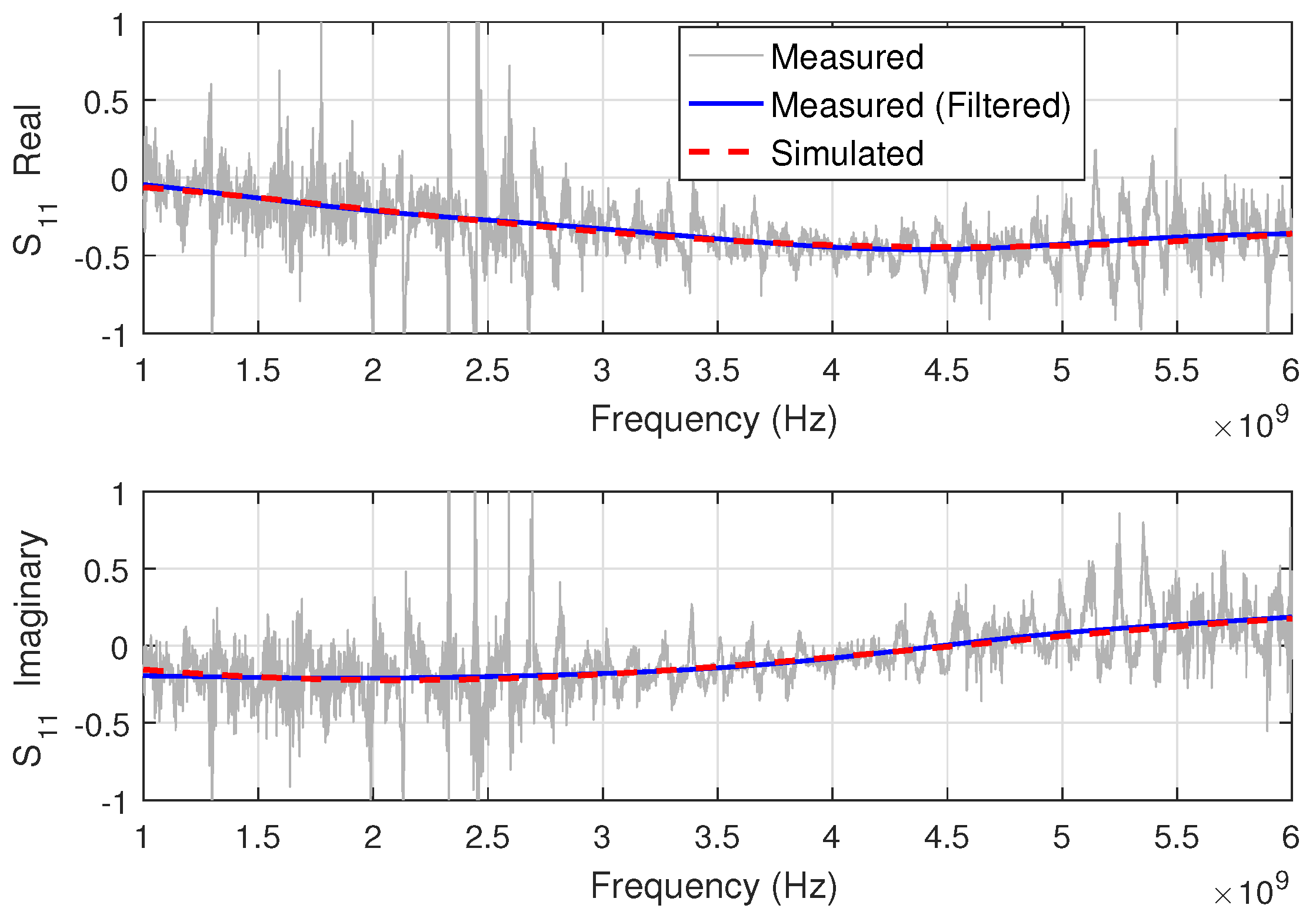
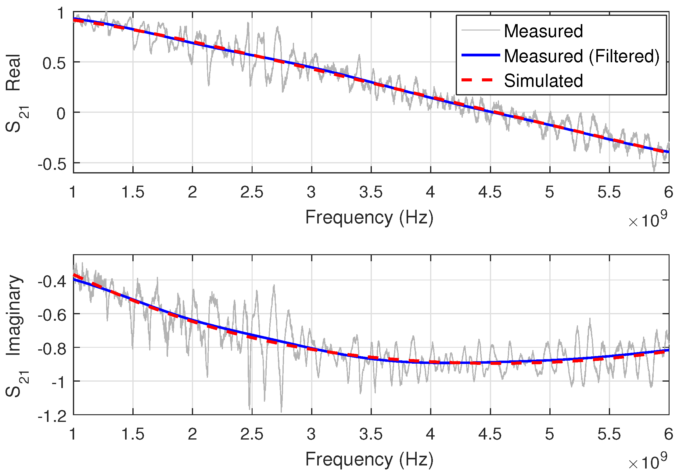
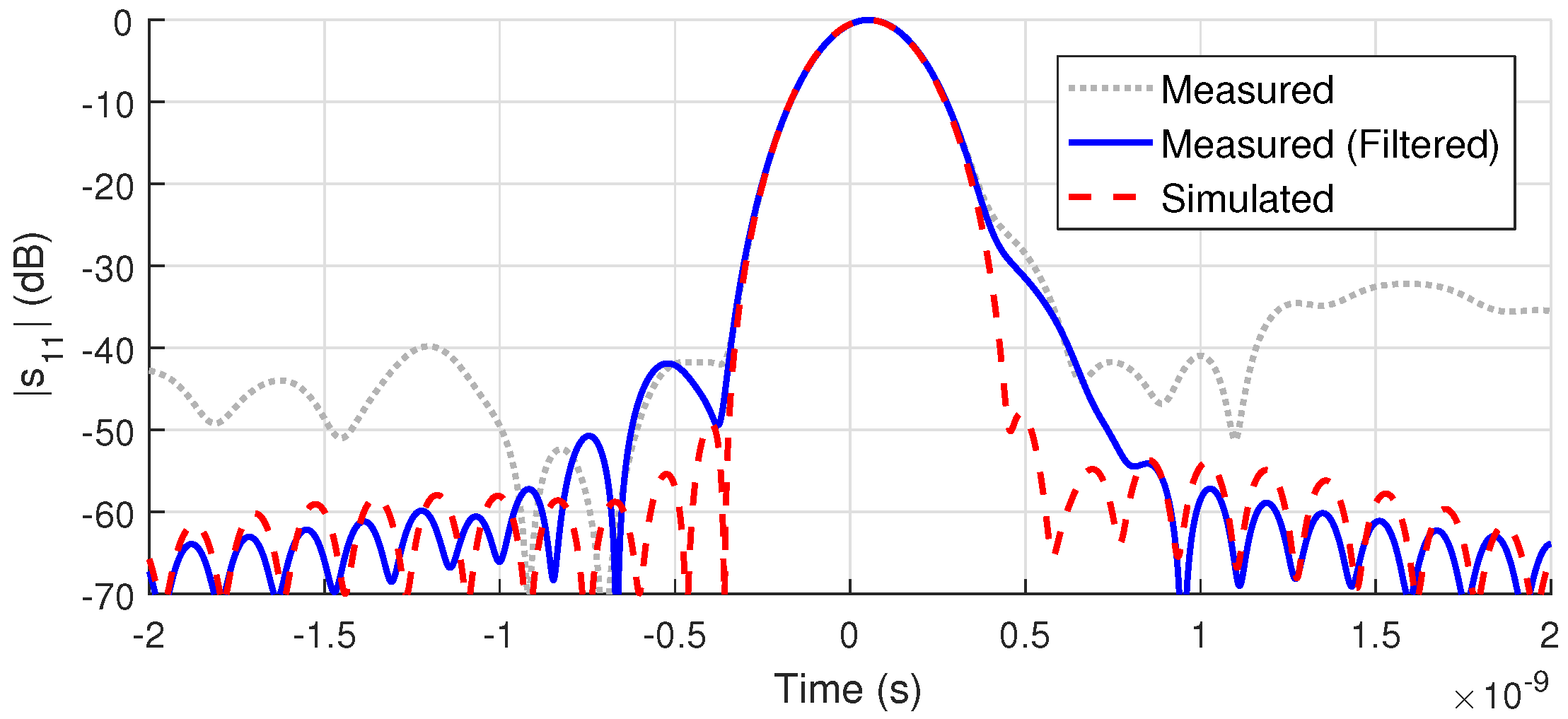
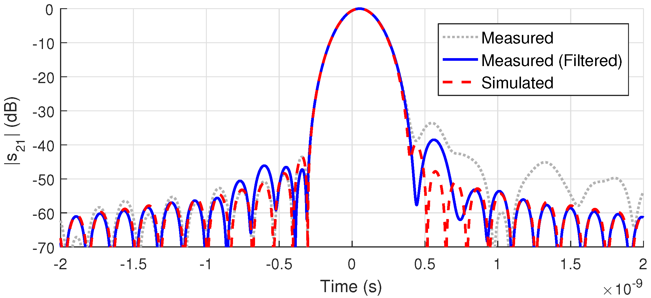
2.6. Filtering the S-Parameters

After the calibration, the S-Parameters mainly represent the sample itself. Despite of that, they are quite noisy, so that a filtering procedure is introduced here. The TDG is applicable for different transmission line setups. It is, however, an optional tool with a specific license in a typical VNA. Other authors have implemented gating codes, for instance [27,30], but yet some details are not much discussed in literature. Our gating algorithm is described in Appendix B, in which a flow chart is used to illustrate the overall process.

In Figure 6 and Figure 7 both the noisy and the filtered measurements referring to $S_{11}$ and $S_{21}$ of a Polymethylmethacrylate (PMMA) sample with $d=10.2$ mm are shown. For comparison, reference signals simulated by (4) and (5) with ${\epsilon }_r=2.61$ and ${\mu }_r=1$ are also reported.

The VNA provides the S-Parameters in frequency-domain (FD), but in many cases it is worthy to analyze them also in time-domain (TD). In this way, one can remove unwanted contributions, criteriously. Due to the multiple reflections and transmissions, we have multiple peaks in TD, with different magnitudes and delays. This separation in TD is useful because it can facilitate the identification of the unwanted contributions. The spreaded noise in Figure 6 and Figure 7, for instance, corresponds to side lobes in TD (see Figure 8 and Figure 9), which can be reduced by a filtering process (gating). Note that in practice this identification is impaired by frequency bandwidth (BW) limitations, since the TD resolution is inversely proportional to BW [1,3].

One should note that it is not necessary to calculate the transform in the whole default range, since we are only interested in the details in the vicinity of the sample. The inverse Chirp Z-Transform (CZT) is then used [47]. It is more general and flexible than the Discrete Fourier Transform (DFT) because it controls the mapping between the domains by an initial point $t_1$ and an increment $\delta t$ [48,49].

Note by Figure 6 and Figure 7 that the filtered data match very well the frequency behavior of the simulated scattering parameters. However, a spurious low-level oscillation is still present due to: (a) the inherent difficulty in sharply separating the noise from the genuine signal when they are too close in TD. In particular, this gets worse when the TD resolution is not so high to avoid overlapping, that is, unresolved peaks; and (b) the gated signal presents errors concentrated on the frequency band edges and also a small oscillation over the whole band [50]. Therefore, a residual distortion is a typical characteristic of gated signals and, in our context, it leads to some distortion on the extracted properties.

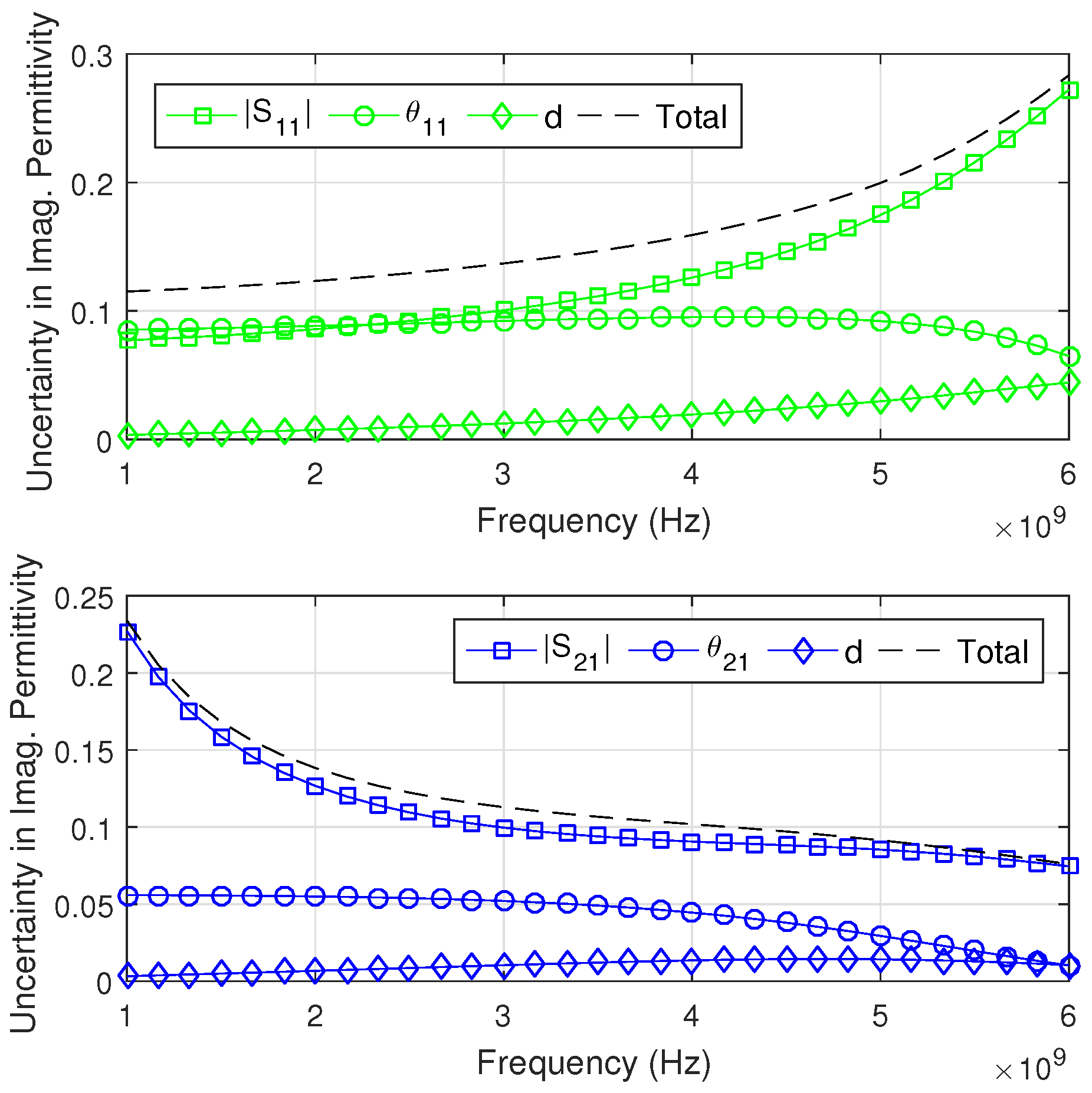
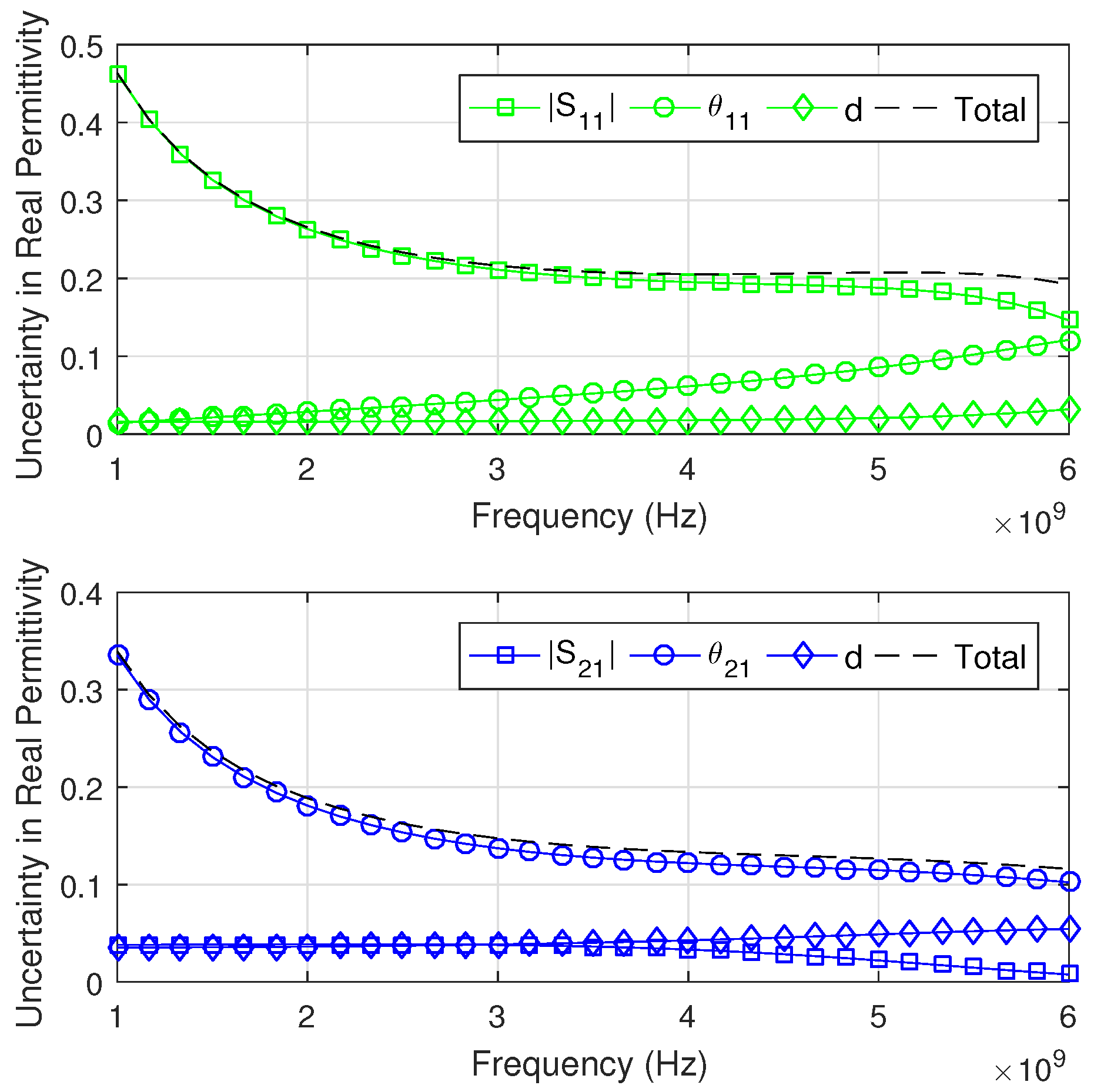
3. Analysis of the Uncertainties in the Model

For the estimation of the uncertainty in the extracted ${\epsilon }_r$ due to the uncertainties in the measured S-Parameters and in the thickness d, we assume ${\mu }_r=1$ and use a differential uncertainty analysis [41]. Then, the total uncertainty in ${\epsilon }_r$ is

$$\Delta {\epsilon }_r^p=\sqrt{{\left({\displaystyle \frac{\partial {\epsilon }_r^p}{\partial |S_m|}}\Delta \left|S_m\right|\right)}^2+{\left({\displaystyle \frac{\partial {\epsilon }_r^p}{\partial {\theta }_m}}\Delta {\theta }_m\right)}^2+{\left({\displaystyle \frac{\partial {\epsilon }_r^p}{\partial d}}\Delta d\right)}^2},$$

(11)

where $\Delta$ means the uncertainty in the respective quantity, ${\theta }_m$ is the phase of $S_m$, $m=$ 11 or 21 and p stands for the real or imaginary part of ${\epsilon }_r$.

Because we do not have an explicit function for ${\epsilon }_r$, the partial derivatives in (11) are calculated using the implicit function theorem [51], after calculating $\partial F_{RO}/\partial \left|S_{11}\right|$, $\partial F_{RO}/\partial {\theta }_{11}$, $\partial F_{RO}/\partial {\epsilon }_r$, $\partial F_{RO}/\partial d$, $\partial F_{TO}/\partial \left|S_{21}\right|$, $\partial F_{TO}/\partial {\theta }_{21}$, $\partial F_{TO}/\partial {\epsilon }_r$ and $\partial F_{TO}/\partial d$. Due to the non linear nature of the involved functions, the total uncertainty depends on the working point. Therefore, in order to quantify (11), we use the VNA specifications [52] and assume that $\Delta d$ is the standard deviation of d, which we measured in different points of the sample.

3.1. Individual Contributions on the Total Uncertainty

For the analysis of the behavior of $\Delta {\epsilon }_r$ as a function of frequency, we fix the evaluation point at ${\epsilon }_r^{\prime }$ = 2.61, ${\epsilon }_r^{″}=0.005$, $d=10.2$ mm. These values are defined based on one of our samples. Additionally, we use the measured thickness uncertainty $\Delta d=0.1$ mm and, for the scattering parameters, $\Delta |S_{11}|=$ 0.05, $\Delta {\theta }_{11}=$ 3${}^{\circ }$, $\Delta |S_{21}|=$ 0.02 and $\Delta {\theta }_{21}=$ 2${}^{\circ }$ [52].

In Figure 10 and Figure 11 the individual contribution of $\Delta |S_m|$, $\Delta {\theta }_m$ and $\Delta d$ to the uncertainty on the real and imaginary part of ${\epsilon }_r$ are shown (lines with markers), together with their total effect (dashed line). In general, we observe that: (a) the major contribution to $\Delta {\epsilon }_r^{\prime }$ is due to $|S_{11}|$ when using reflection and is due to ${\theta }_{21}$ when using transmission (see Figure 10); thus, $S_{11}$ data is very important when ${\theta }_{21}$ is not reliable; (b) the major contribution to $\Delta {\epsilon }_r^{″}$ is due to uncertainties in the magnitude of both the S-Parameters, but their effect as a function of frequency is much different in reflection and transmission configurations, i.e., one increases with f, the other decreases (see Figure 11).

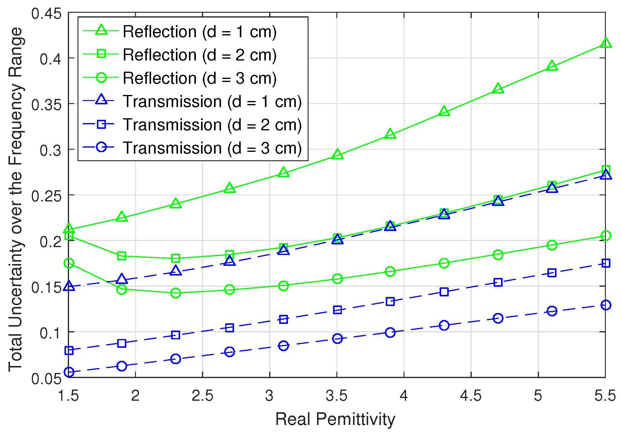
3.2. Uncertainty for Different Materials and Thicknesses

Here we study the uncertainty when the evaluation point in (11) changes. Specifically, we keep fixed ${\epsilon }_r^{″}=0.005$ and make ${\epsilon }_r^{\prime }$ and thickness d vary within a predefined range. In order to simply quantify the uncertainty taking into account the whole frequency range, we defined it as $\Delta {{\epsilon }_r}_{F_{RO}}^f=\sqrt{{\left(\left|\right|\Delta {{\epsilon }_r}_{F_{RO}}{\left|\right|}_f\right)}^2/N_f}$ for $F_{RO}$ and similarly for $F_{TO}$, where $N_f$ is the number of frequency points.

The resulting uncertainty is shown in Figure 12, for reflection data and also for transmission data, that is $\Delta {{\epsilon }_r}_{F_{TO}}^f$ and $\Delta {{\epsilon }_r}_{F_{RO}}^f$, respectively. Three values of thickness d are used. Note that: (a) smaller uncertainties are achieved with thicker samples and using transmission; (b) the uncertainty tends to increase as ${\epsilon }_r^{\prime }$ increases; (c) the curves are quite linear in transmission mode; (d) the most variation is for lower ${\epsilon }_r^{\prime }$ in the reflection mode.

4. Results and Discussion

In this section two materials are used for the measurements: (a) Polytetrafluorethylene (PTFE), and (b) Polymethylmethacrylate (PMMA). The samples are 50 × 50 cm with $d=$ 10.5 mm (PTFE) and $d=$ 10.2 mm (PMMA). The measured standard deviations of d are 1.59% and 0.97%, respectively. Two distances r between the antennas and the sample are considered: 30 cm and 48 cm.

The reported ${\epsilon }_r^{\prime }$ of PTFE in literature is often between 2.03 and 2.05 [1,5,27,33,34,35]. As a reference, we assume that the samples are non-magnetic (${\mu }_r=$ 1.00) and non-dispersive in our range. For the simulations we based on the following properties [35]: PTFE: ${\epsilon }_r^{\prime }=$ 2.05 ± 0.02, ${\epsilon }_r^{″}=$ 0.0002 ± 0.00008; PMMA: ${\epsilon }_r^{\prime }=$ 2.61 ± 0.02, ${\epsilon }_r^{″}=$ 0.005 ± 0.00008.

When TDG is used, it is assumed the suitable set [31]: $N_t=N_f=4001$, ${\Delta }_{fe}=$ 0.5 GHz, $g_{t_1}=-$0.5 ns, $g_{t_2}=+$0.5 ns, 68 dB of sidelobe attenuation and a 0.5 ns cut-off time [28]. Details about these parameters are in Appendix B.

4.1. Frequency-by-Frequency with Simulated Data

Here we use simulated data to validate the extraction with TDG in different SNR scenarios. Arbitrary white gaussian noise has been added to the theoretical S-Parameters with the following SNR: 5, 10 and 20 dB. In order to simplify the study, we set ${\epsilon }_r=$ 2.05 (PTFE), ${\epsilon }_r=$ 2.61 (PMMA) and ${\mu }_r=$ 1.00 for both materials.

The average value and the standard deviation of the recovered properties, over the frequency range, using the three methods under consideration are in

Table 1. Over the frequency average and standard deviation of the extracted properties for the simulated materials, using the frequency-by-frequency approaches with different SNR.

PTFE (NRW)
SNR (dB)	${\epsilon }_r^{\prime }$	${\epsilon }_r^{″}$	${\mu }_r^{\prime }$	${\mu }_r^{″}$
5	2.05 ± 0.04	−0.01 ± 0.07	1.00 ± 0.02	−0.01 ± 0.02
10	2.04 ± 0.02	0.01 ± 0.03	0.99 ± 0.03	0.01 ± 0.01
20	2.04 ± 0.04	0.00 ± 0.02	0.99 ± 0.02	0.00 ± 0.01
PTFE (Reflection) PTFE (Transmission)
SNR (dB)	${\epsilon }_r^{\prime }$	${\epsilon }_r^{″}$	${\epsilon }_r^{\prime }$	${\epsilon }_r^{″}$
5	2.05 ± 0.07	0.00 ± 0.07	2.05 ± 0.03	−0.02 ± 0.08
10	2.05 ± 0.03	0.00 ± 0.04	2.03 ± 0.06	0.02 ± 0.04
20	2.04 ± 0.02	0.00 ± 0.03	2.03 ± 0.06	−0.01 ± 0.02
PMMA (NRW)
SNR (dB)	${\epsilon }_r^{\prime }$	${\epsilon }_r^{″}$	${\mu }_r^{\prime }$	${\mu }_r^{″}$
5	2.61 ± 0.08	0.03 ± 0.1	0.99 ± 0.03	−0.03 ± 0.03
10	2.60 ± 0.04	−0.01 ± 0.04	0.98 ± 0.02	−0.02 ± 0.03
20	2.60 ± 0.04	0.01 ± 0.04	1.00 ± 0.01	0.00 ± 0.01
PMMA (Reflection) PMMA (Transmission)
SNR (dB)	${\epsilon }_r^{\prime }$	${\epsilon }_r^{″}$	${\epsilon }_r^{\prime }$	${\epsilon }_r^{″}$
5	2.58 ± 0.11	0.06 ± 0.12	2.62 ± 0.06	−0.01 ± 0.07
10	2.61 ± 0.06	0.02 ± 0.07	2.60 ± 0.05	−0.03 ± 0.03
20	2.60 ± 0.04	0.01 ± 0.05	2.60 ± 0.05	0.00 ± 0.04

. We can observe that, in general, the standard deviation decreases as the SNR increases. It does not imply, however, that the average value tends to the nominal one, since the TDG may remove not only the noise, but also some genuine information of the signal.

The worst permittivity value obtained for PMMA, that is, the most different with respect to the nominal one, is ${\epsilon }_r^{\prime }=$ 2.58 (5 dB SNR), which is 1.15% lower than the expected value. The worst case for PTFE is ${\epsilon }_r^{\prime }=$ 2.03, that is 1% below the adopted reference. The worst difference in ${\mu }_r^{\prime }$ is 2% for PMMA and 1% for PTFE.

Note that as the method does not restrict the extracted values and the imaginary parts are very small, a variation of the order of ${10}^{-2}$ easily introduces negative values, without physical meaning.

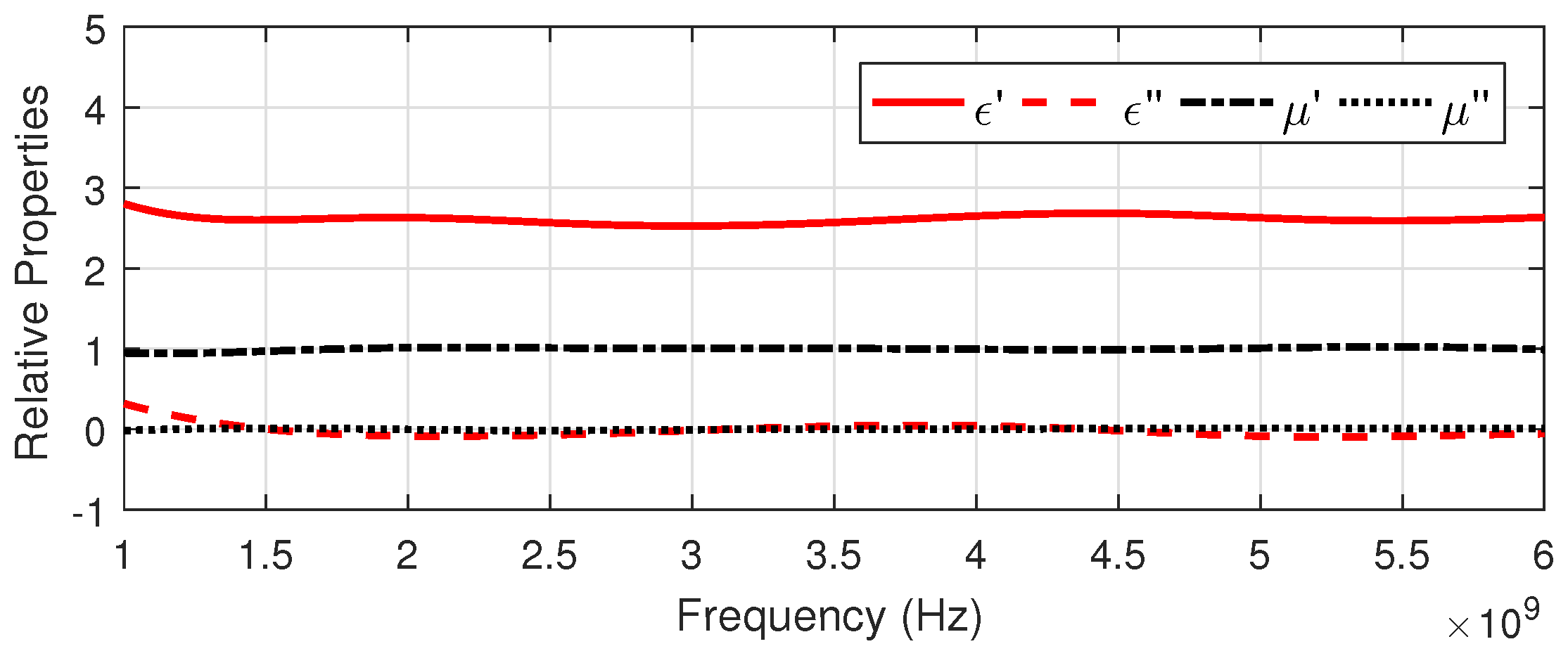
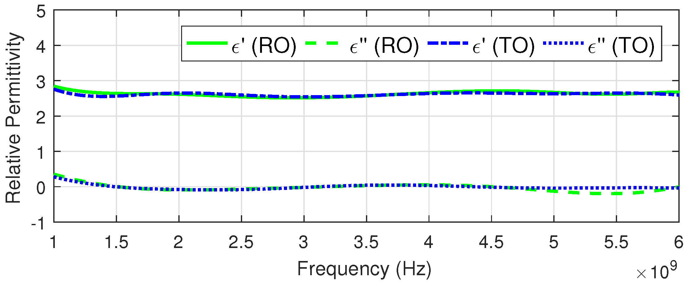
4.2. Frequency-by-Frequency with Experimental Data

The extracted ${\epsilon }_r$ and ${\mu }_r$ of PMMA using the NRW algorithm are in Figure 13, whilst the results for the iterative methods (transmission or reflection) are in Figure 14. It is possible to observe some oscillation on the curves, which is mainly the consequence of using the TDG. The average value over the frequency range and its standard deviation are in

Table 2. The average and the standard deviation of the extracted parameters of the PTFE and PMMA samples, using the frequency-by-frequency approaches in two distances r.

PTFE (NRW)
r	${\epsilon }_r^{\prime }$	${\epsilon }_r^{″}$	${\mu }_r^{\prime }$	${\mu }_r^{″}$
48 cm	2.04 ± 0.03	0.01 ± 0.05	0.98 ± 0.02	0.00 ± 0.01
30 cm	2.04 ± 0.03	−0.03 ± 0.03	0.99 ± 0.02	0.03 ± 0.02
PTFE (Reflection) PTFE (Transmission)
r	${\epsilon }_r^{\prime }$	${\epsilon }_r^{″}$	${\epsilon }_r^{\prime }$	${\epsilon }_r^{″}$
48 cm	2.06 ± 0.04	0.03 ± 0.06	2.01 ± 0.03	0.00 ± 0.04
30 cm	2.08 ± 0.06	−0.06 ± 0.04	2.02 ± 0.04	0.01 ± 0.03
PMMA (NRW)
r	${\epsilon }_r^{\prime }$	${\epsilon }_r^{″}$	${\mu }_r^{\prime }$	${\mu }_r^{″}$
48 cm	2.61 ± 0.05	−0.02 ± 0.07	1.00 ± 0.02	0.00 ± 0.01
30 cm	2.64 ± 0.07	−0.03 ± 0.04	1.01 ± 0.03	0.01 ± 0.01
PMMA (Reflection) PMMA (Transmission)
r	${\epsilon }_r^{\prime }$	${\epsilon }_r^{″}$	${\epsilon }_r^{\prime }$	${\epsilon }_r^{″}$
48 cm	2.62 ± 0.07	−0.03 ± 0.1	2.61 ± 0.04	−0.01 ± 0.06
30 cm	2.66 ± 0.09	−0.06 ± 0.07	2.64 ± 0.06	0.01 ± 0.04

, for different configurations and for both tested materials. For brevity, the results for the PTFE are only in the table.

Because the tested materials are low-loss, the relative uncertainty in the imaginary part is pronounced. Actually, it is also coherent with the fact that free-space methods have a limited capability of measuring imaginary parts lower than 0.01 [5,13,27].

Regarding the two distances, we observe that the results are more consistent when $r=$ 48 cm, especially for PMMA, confirming that the plane-wave premise is quite important in our setup. We should also note that the standard deviations of the extracted properties using experimental data are comparable with those obtained in the simulations, particularly for SNR = 10 or 20 dB.

Regarding the extraction methods, the results for PMMA are more uniform compared with those for PTFE. This can be justified by the higher $\Delta d$ on the PTFE sample and by its possible bending during the calibration (the PTFE sample is not so rigid as the PMMA one, so it bends slightly when supported only by its borders).

It must be noted that the results obtained with the experimental data are better than that expected by the uncertainty analysis. This is due to the fact the errors in the actual measurements are lower than the uncertainties declared by the VNA specifications. In this way, the influence of $\Delta d$ becomes predominant. Additionally, when performing the free-space calibration more uncertainties may be introduced in the data. Note, for instance, that the shift in the phase depends on knowing d. Considering the discussed aspects, in general, the experimental results are in good agreement with simulations and literature.

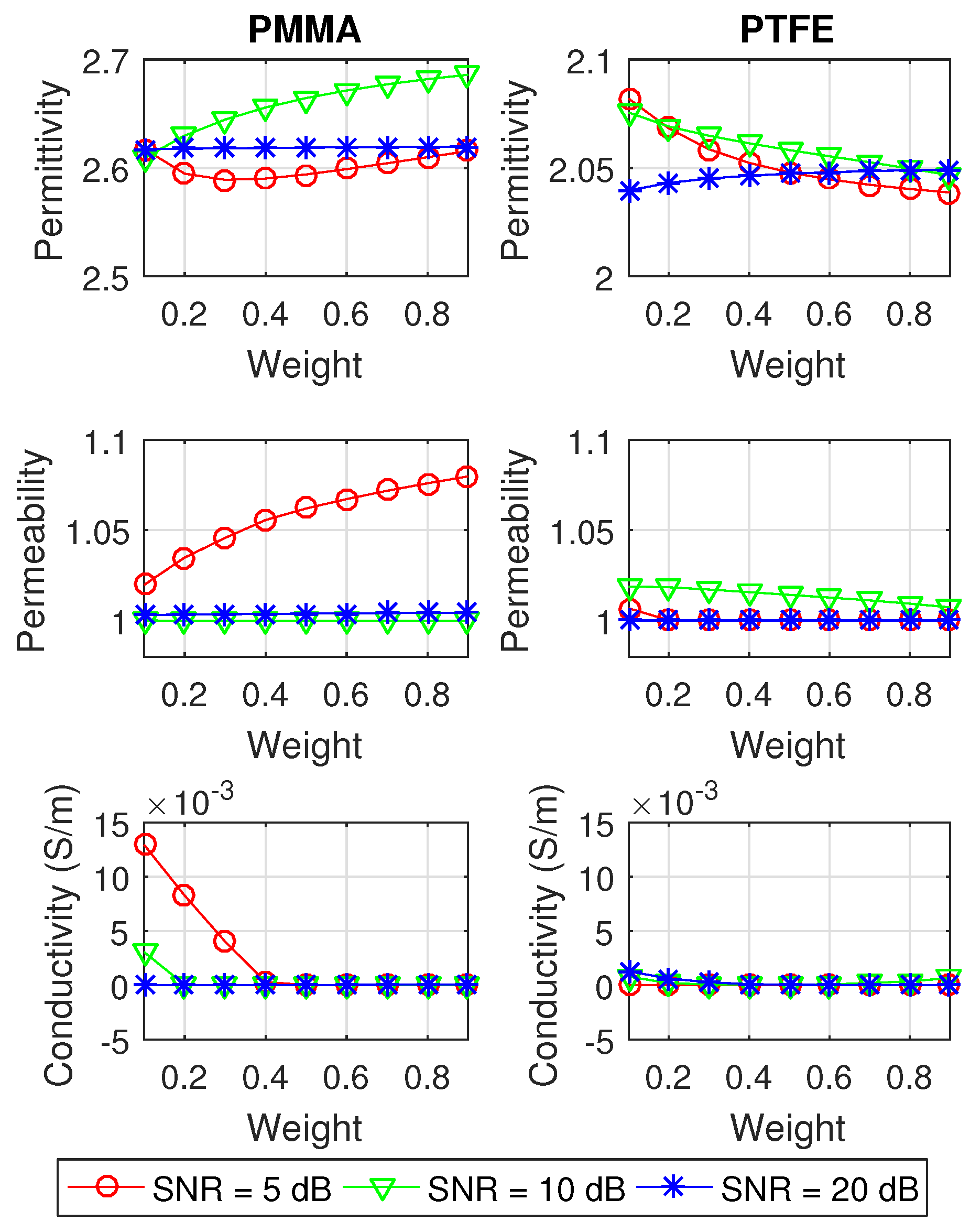
4.3. Multi-Frequency Reconstruction with Simulated Data

Here we simulate the same scenarios of Section 4.1, but with different weights w in (3). Observe that when using $w=$ 0 or 1, either transmission or reflection is used, respectively. The dependence of the scattering parameters on the searched for ${\epsilon }_r$, ${\mu }_r$ and $\sigma$ varies with frequency, providing more or less sensitivity for either $S_{11}$ or $S_{21}$. In order to avoid ill conditioning we limit $0.1\le w\le 0.9$. Thus, we always use both transmission and reflection, but with different weights.

The MATLAB function fmincon is used to minimize $\mathsf{\Psi }$, with the bounds $1\le {\epsilon }_r\le 10$, $1\le {\mu }_r\le 10$ and $0\le \sigma \le 0.1$ S/m; the initial point is ${\epsilon }_r={\mu }_r=1$ and $\sigma =0$. Observe that local minimum can occur, so the choice of the initial point is crucial as we are using a deterministic algorithm. Alternatively, one can use a global search algorithm, which typically increase the computational cost.

The extracted properties of the theoretical samples are in Figure 15. Intuitively, more reliable results are obtained for the higher SNR. In this case, the weight w has less influence, after all, the signals are good. In contrast, in a lower SNR scenario w is, in general, more influent.

4.4. Multi-Frequency Reconstruction with Experimental Data

After the use of theoretical data, we apply the minimization strategy to extract the properties from the experimental S-Parameters, measured with $r=48$ cm. In order to compare the approaches and because the experimental noise in data is not necessarily gaussian, here we test the extraction using the raw signals (without gating) and also using the gated ones.

Table 3. Extracted parameters of the samples using the multi-frequency reconstruction with the measurements performed at distance $r=$ 48 cm, using different weights w in (3).

PTFE (without Gating) PTFE (with Gating)
w	${\epsilon }_r$	${\mu }_r$	$\sigma$ (S/m)	w	${\epsilon }_r$	${\mu }_r$	$\sigma$ (S/m)
0.1	2.03	1.00	0.00	0.1	2.02	1.00	0.00
0.2	2.03	1.00	0.00	0.2	2.03	1.00	0.00
0.3	2.03	1.00	0.00	0.3	2.03	1.00	0.00
0.4	2.03	1.00	0.00	0.4	2.03	1.00	0.00
0.5	2.03	1.00	0.00	0.5	2.03	1.00	0.00
0.6	2.03	1.00	0.00	0.6	2.03	1.00	0.00
0.7	2.04	1.00	0.00	0.7	2.03	1.00	0.00
0.8	2.04	1.00	0.00	0.8	2.04	1.00	0.00
0.9	5.00	2.10	0.00	0.9	4.98	2.44	0.05
PMMA (without Gating) PMMA (with Gating)
w	${\epsilon }_r$	${\mu }_r$	$\sigma$ (S/m)	w	${\epsilon }_r$	${\mu }_r$	$\sigma$ (S/m)
0.1	2.61	1.00	0.00	0.1	2.59	1.01	0.01
0.2	2.61	1.00	0.00	0.2	2.59	1.01	0.01
0.3	2.61	1.00	0.00	0.3	2.59	1.01	0.01
0.4	2.61	1.00	0.00	0.4	2.59	1.01	0.01
0.5	2.61	1.00	0.00	0.5	2.59	1.01	0.01
0.6	2.61	1.00	0.00	0.6	2.59	1.01	0.01
0.7	2.61	1.00	0.00	0.7	2.59	1.01	0.01
0.8	2.61	1.00	0.00	0.8	2.59	1.01	0.01
0.9	2.61	1.00	0.00	0.9	5.00	1.72	0.17

summarizes the extracted properties for both samples, for different w, with and without gating. In some cases the results for different w vary in the order of ${10}^{-3}$ or less, so the rounded values at the table are the same. Such a weak dependence on w indicates that our measured data perform similar to simulated high SNR data.

We observe that $w=$ 0.9 can give wrong solutions due to local minima presence. A simple inspection of the value of $\mathsf{\Psi }$ can help in discarding abnormal solutions. One should, therefore, test different weights w in order to detect the occurrence of a local minimum.

The extracted properties are quite good and we see that, indeed, the TDG seems to be not necessary when using this approach. This is because, in a certain sense, the minimization of the functional $\mathsf{\Psi }$ acts like a filter. Actually, not using the gate in PMMA achieved better results.

The better results achieved by the multi-frequency approach are due to the a priori assumption that the material is non dispersive, so that its properties are constant with frequency and all the measured data, as a whole, contributes to the final results. Conversely, the frequency-by-frequency approach exploits each data individually, so that it has “less information” at disposal. The counterpart, of course, is that it can treat dispersive materials without the need of knowing the model.

5. Conclusions

In this paper we explored two complementary approaches for extracting the properties of materials using a free-space experimental setup. The presented system avoids the cost of an anechoic environment and the costs of commercial solutions for post-processing and extraction.

The implemented Time-Domain Gating has proven to be an useful tool when using frequency-by-frequency approaches, filtering out much of the interferences that affect the free-space measurements. Some advantages of an TDG implementation are: (a) an algorithm more flexible than proprietary solutions, (b) equipment independent, (c) no costs, and (d) useful for research and academic purposes.

A differential uncertainty analysis has been presented to quantify the influence of measured data and slab thickness uncertainties in the final results. The extracted properties are in good agreement with the theoretical ones. Variations in the experimental results are, in general, consistent with those obtained with simulation, which indicates that the measurement setup can indeed provide good data, despite not having electromagnetic absorbers or a sophisticated positioning system.

Results are consistent within the hundredth, but the relative error in the imaginary part is significant when dealing with low loss materials. This is also consistent with the expectation that such small imaginary parts are difficult to be measured by free-space methods.

The multi-frequency approach has proven to be more robust with respect to noisy data. We validate its applicability to FSM, with non gated experimental data. In general, it is preferable using the two S-Parameters, since it can avoid worse results and under-determination when one of them is low. On the other hand, the frequency-by-frequency approach does not make use of restrictions, so that it can be applied to dispersive materials straightforwardly.

In order to improve the measurement system, some topics for further investigations are: (a) using the additional data $S_{12}$ and $S_{22}$ to increase the robustness of the measurements; (b) testing dispersive materials in the measurement band; (c) optimizing the gate parameters and the variables d and $L_1$.

References

1. Chen, L.; Ong, C.; Neo, C.; Varadan, V.V.; Varadan, V.K. Microwave Electronics—Measurement and Materials Characterization; John Wiley & Sons, Inc.: Hoboken, NJ, USA, 2004. [Google Scholar]
2. Balanis, C.A. Advanced Engineering Electromagnetics, 3rd ed.; John Wiley & Sons, Inc.: Hoboken, NJ, USA, 2012. [Google Scholar]
3. Hiebel, M. Fundamentals of Vector Network Analysis, 5th ed.; Rohde & Schwarz: Munich, Germany, 2011. [Google Scholar]
4. Costa, F.; Borgese, M.; Degiorgi, M.; Monorchio, A. Electromagnetic Characterisation of Materials by Using Transmission/Reflection (T/R) Devices. Electronics 2017, 6, 95. [Google Scholar] [CrossRef]
5. Ghodgaonkar, D.K.; Varadan, V.V.; Varadan, V.K. A Free-space Method for Measurement of Dielectric Constants and Loss Tangents at Microwave Frequencies. IEEE Trans. Instrum. Meas. 1989, 37, 789–793. [Google Scholar] [CrossRef]
6. William, S.W.; Alberto, S. Measurement of Dielectric Material Properties—Application Note; Rohde & Schwarz: Munich, Germany, 2006. [Google Scholar]
7. Varadan, V.V.; Hollinger, R.D.; Ghodgaonkar, D.K.; Varadan, V.K. Free-space, broadband measurements of high-temperature, complex dielectric properties at microwave frequencies. IEEE Trans. Instrum. Meas. 1991, 40, 842–846. [Google Scholar] [CrossRef]
8. Jose, K.A.; Varadan, V.K.; Varadan, V.V. Wideband and noncontact characterization of the complex permittivity of liquids. Microw. Opt. Technol. Lett. 2001, 30, 75–79. [Google Scholar] [CrossRef]
9. Brancaccio, A.; D’Alterio, G.; Stefano, E.D.; Guida, L.D.; Feo, M.; Luce, S. A free-space method for microwave characterization of materials in aerospace application. In Proceedings of the MetroAeroSpace 2014, Benevento, Italy, 29–30 May 2014. [Google Scholar]
10. Zaki, F.M.; Awang, Z.; Baba, N.H.; Zoolfakar, A.S.; Bakar, R.A.; Zolkapli, M.; Fadzlina, N. A free-space method for measurement of complex permittivity of double-layer dielectric materials at microwave frequencies. In Proceedings of the 2010 IEEE Student Conference on Research and Development (SCOReD), Putrajaya, Malaysia, 13–14 December 2010. [Google Scholar] [CrossRef]
11. Ozbay, E.; Aydin, K.; Cubukcu, E.; Bayindir, M. Transmission and Reflection Properties of Composite Double Negative Metamaterials in Free Space. IEEE Trans. Antennas Propag. 2003, 51, 2592–2595. [Google Scholar] [CrossRef]
12. Seo, I.S.; Chin, W.S.; Lee, D.G. Characterization of electromagnetic properties of polymeric composite materials with free space method. Compos. Struct. 2004, 66, 533–542. [Google Scholar] [CrossRef]
13. Chung, J.Y. Broadband Characterization Techniques for RF Materials and Engineered Composites. Ph.D. Thesis, Ohio State University, Columbus, OH, USA, 2010. [Google Scholar]
14. Hock, K.M. Error correction for diffraction and multiple scattering in free-space microwave measurement of materials. IEEE Trans. Microw. Theory Technol. 2006, 54, 648–659. [Google Scholar] [CrossRef]
15. Cuinas, I.; Sanchez, M.G. Building material characterization from complex transmissivity measurements at 5.8 GHz. IEEE Trans. Antennas Propag. 2000, 48, 1269–1271. [Google Scholar] [CrossRef]
16. Luo, Q.; Wang, X.; Huang, K.; Li, X.; Zhang, S. A Practical Evaluation Method of Building Penetration Loss at 3.5 GHz for IMT Application. In Proceedings of the 2017 9th International Conference on Measuring Technology and Mechatronics Automation (ICMTMA), Changsha, China, 14–15 January 2017; pp. 150–153. [Google Scholar] [CrossRef]
17. Hasar, U. Non-destructive testing of hardened cement specimens at microwave frequencies using a simple free-space method. NDT E Int. 2009, 42, 550–557. [Google Scholar] [CrossRef]
18. Solimene, R.; Napoli, R.D.; Soldovieri, F.; Pierri, R. TWI for an unknown symmetric lossless wall. IEEE Trans. Geosci. Remote Sens. 2011, 49, 2876–2886. [Google Scholar] [CrossRef]
19. Brancaccio, A.; Soldovieri, F.; Leone, G.; Sglavo, D.; Pierri, R. Microwave characterization of materials in civil engineering. Proc. EUMA 2006, 2, 128–135. [Google Scholar]
20. Arunachalam, K.; Melapudi, V.; Udpa, L.; Udpa, S. Microwave NDT of cement-based materials using far-field reflection coefficients. NDT E Int. 2006, 39, 585–593. [Google Scholar] [CrossRef]
21. Denoth, A. Structural phase changes of the liquid water component in Alpine snow. Cold Reg. Sci. Technol. 2003, 37, 227–232. [Google Scholar] [CrossRef]
22. Trabelsi, S.; Nelson, S.O. Free-Space Measurement of Dielectric Properties of Cereal Grain and Oilseed as Microwave Frequencies. IOP Meas. Sci. Technol. 2003, 14, 589–600. [Google Scholar] [CrossRef]
23. Friedsam, G.L.; Biebl, E.M. A broadband free-space dielectric properties measurement system at millimeter wavelengths. IEEE Trans. Instrum. Meas. 1997, 46, 515–518. [Google Scholar] [CrossRef]
24. Suzuki, H.; Nishikata, A.; Higashida, Y.; Takahashi, T.; Hashimoto, O. Free space method with parallel electromagnetic wave beam by using dielectric lenses and horn antennas for reflectivity of electromagnetic absorbers in millimeter waves. In Proceedings of the 2005 IEEE International Workshop on Measurement Systems for Homeland Security, Contraband Detection and Personal Safety Workshop, Orlando, FL, USA, 29–30 March 2005; pp. 63–69. [Google Scholar] [CrossRef]
25. Hassan, A.M.; Obrzut, J.; Garboczi, E.J. A Q-Band Free-Space Characterization of Carbon Nanotube Composites. IEEE Trans. Microw. Theory Technol. 2016, 64, 3807–3819. [Google Scholar] [CrossRef] [PubMed]
26. Collier, R.; Skinner, D. (Eds.) Microwave Measurements, 3rd ed.; IET Electrical Measurement Series; The Institution of Engineering and Technology: Stevenage, UK, 2007. [Google Scholar]
27. Amiet, A. Free Space Permittivity and Permeability Measurements at Microwave Frequencies. Ph.D. Thesis, Monash Univercity, Melbourne, Australia, 2003. [Google Scholar]
28. Time Domain Analysis Using a Network Analyzer—Application Note 1287-12; Agilent Technologies: Santa Clara, CA, USA, 2012.
29. Time Domain Measurements Using Vector Network Analyzers—Application Note No. 11410-00206, Rev. D; Anritsu: Kanagawa Prefecture, Japan, 2009.
30. Condori-Arapa, C. Antenna Elements Matching—Time Domain Analysis. Master’s Thesis, Gävle University College, Gävle, Sweden, 2010. [Google Scholar]
31. Gonçalves, F.J.F.; Mesquita, R.C.; Silva, E.J. Implementing a Time-Domain Filter for Extracting the Electromagnetic Constitutive Properties. In Proceedings of the MOMAG, João Pessoa, Brazil, 5–8 August 2012. [Google Scholar]
32. Baker-Jarvis, J.; Geyer, R.G.; Domich, P.D. A nonlinear least-squares solution with causality constraints applied to transmission line permittivity and permeability determination. IEEE Trans. Instrum. Meas. 1992, 41, 646–652. [Google Scholar] [CrossRef]
33. Nicolson, A.M.; Ross, G.F. Measurement of the Intrinsic Properties of Materials by Time-Domain Techniques. IEEE Trans. Instrum. Meas. 1970, 19, 377–382. [Google Scholar] [CrossRef]
34. Weir, W.B. Automatic Measurement of Complex Dielectric Constant and Permeability at Microwave Frequencies. Proc. IEEE 1974, 62, 33–36. [Google Scholar] [CrossRef]
35. Baker-Jarvis, J.; Janezic, M.D.; Riddle, B.F.; Johnk, R.T.; Kabos, P.; Holloway, C.L.; Geyer, R.G.; Grosvenor, C.A. Measuring the Permittivity and Permeability of Lossy Materials: Solids, Liquids, Metals, Building Materials, and Negative-Index Materials; Technical Note 1536; NIST—National Institute of Standards and Technology: Gaithersburg, MD, USA, 2005. Available online: https://www.nist.gov/publications/measuring-permittivity-and-permeability-lossy-materials-solids-liquids-metals-and (accessed on 12 September 2018).
36. Boughriet, A.H.; Legrand, C.; Chapoton, A. Noniterative Stable Transmission/Reflection Method for Low-Loss Material Complex Permittivity Determination. IEEE Trans. Microw. Theory Technol. 1997, 45, 52–57. [Google Scholar] [CrossRef]
37. Balanis, C.A. Anntena Theory—Analysis and Design, 2nd ed.; John Wiley & Sons: Hoboken, NJ, USA, 1997. [Google Scholar]
38. Dhondt, G.; Zutter, D.D.; Martens, L. An improved free-space technique modelling for measuring dielectric properties of materials. In Proceedings of the 1996 Digest IEEE Antennas and Propagation Society International Symposium, Baltimore, MD, USA, 21–26 July 1996. [Google Scholar]
39. Bartley, P.G.; Begley, S.B. Improved Free-Space S-Parameter Calibration. In Proceedings of the 2005 IEEE Instrumentationand Measurement Technology Conference, Ottawa, ON, Canada, 16–19 May 2005. [Google Scholar]
40. Bartley, P.G.; Begley, S.B. A new free-space calibration technique for materials measurement. In Proceedings of the Instrumentation and Measurement Technology Conference, Graz, Austria, 13–16 May 2012; pp. 47–51. [Google Scholar] [CrossRef]
41. Baker-Jarvis, J.; Vanzura, E.J.; Kissick, W.A. Improved Technique for Determining Complex Permittivity with the Transmission/Reflection Method. IEEE Trans. Microw. Theory Technol. 1990, 38, 1096–1102. [Google Scholar] [CrossRef]
42. Jebbor, N.; Bri, S.; Sánchez, A.; Chaibi, M. A fast calibration-independent method for complex permittivity determination at microwave frequencies. Measurement 2013, 46, 2206–2209. [Google Scholar] [CrossRef]
43. Hasar, U.C. Thickness-Invariant Complex Permittivity Retrieval from Calibration-Independent Measurements. IEEE Microw. Wirel. Compon. Lett. 2017, 27, 201–203. [Google Scholar] [CrossRef]
44. Hasar, U.C. Determination of Complex Permittivity of Low-Loss Samples From Position-Invariant Transmission and Shorted-Reflection Measurements. IEEE Trans. Microw. Theory Technol. 2018, 66, 1090–1098. [Google Scholar] [CrossRef]
45. Akhter, Z.; Akhtar, M.J. Free-Space Time Domain Position Insensitive Technique for Simultaneous Measurement of Complex Permittivity and Thickness of Lossy Dielectric Samples. IEEE Trans. Instrum. Meas. 2016, 65, 2394–2405. [Google Scholar] [CrossRef]
46. Deng, L.; Chen, X.L.; Li, Y. S-parameters extraction of a desired network with time-domain gates. Progress Electromagn. Res. Lett. 2016, 61, 91–97. [Google Scholar] [CrossRef]
47. Rabiner, L.R.; Schafer, R.W.; Rader, C.M. The Chirp Z-Transform Algorithm and Its Application. Bell Syst. Tech. J. 1969, 1249–1292. [Google Scholar] [CrossRef]
48. Oppenheim, A.V.; Schafer, R.W. Discrete-Time Signal Processing; Pearson: London, UK, 2010. [Google Scholar]
49. Smith, S.W. Digital Signal Processing—A Practical Guide for Engineers and Scientists; Newnes: Wolgan Valley, NSW, Australia, 2003. [Google Scholar]
50. I Yagüe, R.D.P.D.; Ibars, A.B.; Martínez, L.F. Analysis and Reduction of the Distortions Induced by Time-Domain Filtering Techniques in Network Analyzers. IEEE Trans. Instrum. Meas. 1998, 47, 930–934. [Google Scholar] [CrossRef]
51. Silov, G. Analisi Matematica—Funzioni di più Variabili Reali, 1st ed.; Edizioni MIR: Moscow, Russia, 1979. [Google Scholar]
52. R&S ZVL Vector Network Analyzer Specifications PD 5213.8150.22, Version 10.00; Technical Report; Rohde & Schwarz: Munich, Germany, 2017.
53. Lu, K.; Brazil, T.J. A systematic error analysis of HP 8510 time-domain gating techniques with experimental verification. In Proceedings of the IEEE MTT-S International Microwave Symposium Digest, Atlanta, GA, USA, 14–18 June1993; pp. 1259–1262. [Google Scholar] [CrossRef]
54. Harris, F.J. On the Use of Windows for Hamonic Analysis with the Discrete Fourier Transform. Proc. IEEE 1978, 66, 51–83. [Google Scholar] [CrossRef]
Figure 1. Representation of the transmission and reflection Free-Space Method. The sample is placed between two antennas, which are connected to the ports of the VNA.
Electronics 07 00260 g001
Figure 2. Extraction of the permittivity ε r and permeability μ r from the S-Parameters S 11 and S 21 .
Electronics 07 00260 g002
Figure 3. The sketch (left) and a photograph (right) of the experimental setup.
Electronics 07 00260 g003
Figure 4. The three configurations used in the free-space calibration: (a) metal plate, (b) air, and (c) material under test. The arrows indicate possible contributions on the measurements.
Electronics 07 00260 g004
Figure 5. Representation of the ticknesses d and L 1 , which are used to adjust the phase.
Electronics 07 00260 g005
Figure 6. S 11 ( ω ) of the PMMA (simulated and measured).
Electronics 07 00260 g006
Figure 7. S 21 ( ω ) of the PMMA (simulated and measured).
Electronics 07 00260 g007
Figure 8. | s 11 ( t ) | of the PMMA (simulated and measured).
Electronics 07 00260 g008
Figure 9. | s 21 ( t ) | of the PMMA (simulated and measured).
Electronics 07 00260 g009
Figure 10. The uncertainty in the real part of permittivity ( Δ ε r ) due to the uncertainties in the magnitude and phase of the S-Parameters and in the thickness d. The reflection configuration is on the top, whilst the transmission is on the bottom.
Electronics 07 00260 g010
Figure 11. The uncertainty in the imaginary part of permittivity ( Δ ε r ) due to the uncertainties in the magnitude and phase of the S-Parameters and in the thickness d. The reflection configuration is on the top; the transmission is on the bottom.
Electronics 07 00260 g011
Figure 12. Total uncertainty over frequency Δ ε r F R O f (solid lines) and Δ ε r F T O f (dashed lines), for different thicknesses d and ε r . The different markers distinguish the thickness d.
Electronics 07 00260 g012
Figure 13. The properties of PMMA extracted by the NRW using experimental data with r = 48 cm.
Electronics 07 00260 g013
Figure 14. The permittivity of PMMA extracted using Reflection Only (RO) and Transmission Only (TO) methods, using experimental data with r = 48 cm.
Electronics 07 00260 g014
Figure 15. The extracted properties of the theoretical samples, for different SNR and weights w. The simulation for PMMA are on the (left), whereas for PTFE are on the (right).
Electronics 07 00260 g015