Estimated Reaction Force-Based Bilateral Control between 3DOF Master and Hydraulic Slave Manipulators for Dismantlement

Abstract

This paper proposes a novel bilateral control design based on an estimated reaction force without a force sensor for a three-degree of freedom hydraulic servo system with master–slave manipulators. The proposed method is based upon sliding mode control with sliding perturbation observer (SMCSPO) using a bilateral control environment. The sliding perturbation observer (SPO) estimates the reaction force at the end effector and second link without using any sensors. The sliding mode control (SMC) is used as a bilateral controller for the robust position tracking and control of the slave device. A bilateral control strategy in a hydraulic servo system provides robust position and force tracking between master and slave. The difference between the reaction force of the slave produced by the effect of the remote environment and the operating force applied to the master by the operator is expressed in the target impedance model. The impedance model is applied to the master and allows the operator to feel the reaction force from the environment. This research experimentally verifies that the slave device can follow the trajectory of the master device using the proposed bilateral control strategy based on the estimated reaction force. This technique will be convenient for three or more degree of freedom (DOF) hydraulic servo systems used in dismantling nuclear power plants. It is worthy to mention that a camera is used for visual feedback on the safety of the environment and workspace.

1. Introduction

This is an era for computer science and technology; thus, automation and remote operation requires time. The automated/remote system must consider, in detail, the manual operation to come up with an alternative solution that provides better control for the operator with instrumental feedback. Several conditions need to be considered when designing and implementing remote activities. These conditions include a clear workspace for designed equipment, the environmental conditions of the area of operation, handling of different types of materials, tool setup and change out among others. The crux of the story is to replace manual tools with a suitable remote system. A simple example is to modify grip operation by utilizing the end effector and implementing remote alignment and pinning methods and using self-standing bails. A successful remote design always inherits a defined workspace for equipment with minimum mechanical limitations to accomplish a task. Remote technology is a broader area that could be subdivided into different fields such as dismantling equipment, cutting tools, segmenting, sampling and workspace to handle the designed equipment. This field has some state-of-the-art applications, e.g., dismantling of nuclear facilities which require more safety. Several articles in past research [1,2,3,4,5,6,7,8] have been published to address this problem. The Maestro robot system was developed in France to dismantle inactive nuclear reactors [9,10].

An alternative for such activities is tele-operation systems which have human control to ensure safety. In tele-operated systems, human personnel set visual/instrumental feedback from the manipulator to decide future tasks. The controller, in this case, acts according to the master–slave configuration. Bilateral control architecture is at favorable positions for such targets, and most research has presented two-channel architecture such as position–position (P-P), position–force (P-F), force–force (F-F) and force–position (F-P). Several other authors in the past [11,12,13,14] have presented bilateral controllers with more than a two-channel architecture.

Several researchers in the past have discussed the improvement in control architecture and the performance of controllers [15,16]. Yana et al. [17] have addressed the finite-time control problem for the bilateral tele-operated environment through resulting feedback. They proposed an observer to estimate a velocity profile by ensuring semi-global stability depending upon the resulting velocity error. A promising feature of this method is that it only utilizes position information which forces the master–slave synchronization error to approach null value in a defined time. Dinh et al. [18] have presented the idea of utilizing a joystick controller to be used for construction machinery control. The authors proposed a controller that is comprised of a force-reflecting gain tuner and a couple of adaptive controllers, namely, master and slave. They implemented a fuzzy logic technique to design local adaptive controllers. Additionally, they utilized an efficient optimization algorithm that provides a real feeling of interaction for an operator at a remote site. Ollin et al. [19] introduced the idea of communications delayed under-actuated mechanical systems under master–slave tele-operated control. They proposed a solution resulting in a particular compiling matrix that ensures the error dynamics refrained in the linear and non-linear parts inherit the matching condition to be satisfied. Later, these linear and non-linear parts are utilized to design discontinuous casual controllers to achieve bilateral co-ordination in position and time. Rabah et al. [20] proposed the idea of using a two adaptive fuzzy controller. The proposed algorithm not only adjusts membership function by the compensatory fuzzy controller but also implements a compensatory learning algorithm for optimal solutions. The first controller is designed under a compensatory neural–fuzzy interface whereas the other is designed under a compensatory adaptive neural–fuzzy interface system. The force–position scheme is utilized by incorporating a two-channel bilateral tele-operated architecture. Finally, the stability and transparency analysis is carried out under passivity framework [20]. Another design of a bilateral controller is presented in Umar et al. [21]. The design is based upon the state of convergence and was implemented for tele-operated systems. The authors applied Takagi–Sugeno’s (TS) fuzzy model approach for approximation. The authors mentioned that SC-based bilateral controllers have several advantages in modeling and control design. The most advantageous feature is the ease to implement. The master–slave system in the modeling step can be performed by an n-th order differential equation. Similarly, its control design step can easily identify the gains required for the desired closed loop dynamics for a particular system.

Another novel control strategy is presented in [22], where the controller is not placed with the system under experiment. The authors analyzed the stability and transparency of the proposed tele-operators. They implemented PD-like controllers for fixed-time delays and P-like controllers for time-varying delays. Another interesting study by Kamran et al. [23], which utilizes a robust controller for master control and an adaptive back-stepping controller is designed for the slave controller. The authors analyzed the scenarios of input-delay uncertainties in the parameters and multi-objective optimization in implementing the robust master control. KD et al. [24] presented the estimating methodology of reaction force for assembly work with a robot manipulator consisting of a three-link dual-arm. They utilized sliding mode control with a sliding perturbation observer. In another study by Tayfun et al. [25], the authors presented bilateral control of a tele-operated system consisting of one master and two-slave systems. The master system was a 6DOF haptic robot while one of the slave systems was a virtual 6DOF robot and another real industrial robot. A visual user interface was created to show the position and velocity profile for tele-operated control. They implemented Lyapunov stability methodology to analyze stability and position localization. Shafiqul et al. [26] investigated a bilateral control tele-operated scheme for a robotic system with unsymmetrical time-varying delays. The authors implemented an adaptive algorithm to determine relating factors between human and master manipulator and between slave and remote setup. Later, delayed estimated factors are fed back to the master and slave systems. The authors estimated and analyzed the impedance properties of the interaction between the human-based system and the remote environment. Further application of bilateral control are electro-pneumatic actuators and mobile robot [27,28].

Xiao et al. [29] presented the model mediated tele-operated approach. This proposed scheme has been designed to achieve stability and transparency while considering the random communication delays. Da Sun et al. [30], proposed a novel approach for tele-operated systems utilizing an extended prescribed performance control and a wave-based time domain passivity scheme. This scheme ensures synchronization of velocity, force, and localization. The stability and performance of the system are analyzed by the standard Lyapunov scheme. This methodology also ensures high tracking results of localization, velocity, and force. Similarly Azimifar et al. [31] presented a strategy to estimate the external force acting on master and slave systems. This scheme is advantageous with low-cost features and ease of implementation as the force sensors requirement is eliminated. They proposed a novel control for a nonlinear bilateral tele-operated system with time delays that estimates the force accordingly. The stability of the system is analyzed through the famous Lyapunov stability methodology. The tele-operation of remote system falls under the umbrella of bilateral control. It includes a master robot system that is operated by human operators and controlled through electric actuators whereas a slave robot system that is placed or installed at a remote location and is controlled through hydraulic actuators. Thus, to achieve an efficient bilateral control, three key features are necessary. The first is the coordinated control that is responsible for decoupling of position and force controllers. Second, is the linearization of hydraulic actuators. Third, is the agreement of system order of electric and hydraulic actuators by using a pseudo differentiator. Sho et al. [32] proposed a novel method with an efficient and accurate tracking performance and is the most stable in a contact control scenario among all three controllers.

Minou et al. [33] proposed a hybrid control algorithm for trajectory tracking with constant force. A non-linear model is implemented for the position controller to achieve predictive tracking, satisfying the input constraints. The authors analyzed the performance of the proposed controller and concluded that position tracking has a proof-mean-square-error (RMSE) of 0.89 mm whereas the catheter regulated the force with RMSE of 4.9 mN. Yaoyao et al. [34] presented a novel idea of trajectory control of an underwater vehicle-manipulator system by implementing a discrete time delay estimating methodology. Xia et al. [35] proposed a non-linear adaptive control algorithm for a non-linear manipulator system with uncertainties in its dynamics. Their algorithm guarantees accurate and efficient tracking. The proposed algorithm not only estimates the manipulator’s dynamics but also determines the best fit dead-zone parameter in adaptation law. The estimated values are later used in proposed control law. The authors claimed and showed results suggesting that tracking is accurate and efficient even when both dynamics and dead-zone uncertainties appear at the same time. There are several studies in the literature which have presented the idea of utilizing force sensors to detect the outer forces in conventional bilateral control schemes, but such addition of force sensors has certain problems. A simple explanation to it is that a manipulator system with a force sensor acts as a two-mass resonant system. Thus, it is a bottleneck in realizing high-frequency force sensing [36,37]. The master and slave configuration of a manipulator system is highly applicable and suitable for nuclear power plants, because of restricted human access. In addition to this, it also requires exact control and dismantling/handling of a material/object with excessive load. Hydraulic systems are best suitable for such an application as they offer high power actuators.

In keeping a view of the above studies, in this study, we implemented the sliding mode control with sliding perturbation observer (SMCSPO). It is an efficient and robust control algorithm that not only estimates the reaction force of master and slave but also determines the bilateral control of the hydraulic servo system of a 3DOF master–slave robot. The reason for using a hydraulic servo system is that its power-to-weight ratio is better than any other type of actuated robot at the expense of positional accuracy. In this study, the sliding perturbation observer (SPO) is implemented to estimate the reaction force of the slave without using any sensor. The bilateral control scheme is implemented for efficient and accurate position and force tracking b/w master–slave configuration with visual feedback. In the bilateral controller, the difference of reaction force of the slave manipulator and operating force applied to the master manipulator is designed to target the impedance model. The reaction force of the slave is resultant of effects in the remote environment while operator force is applied by the operator (Human) at the master manipulator. The experimental results of studies endorse that the slave efficiently follows the position trajectory of the master system.

The manuscript is organized as follows: Section 2 of this paper presents the mechanical structure and dynamics of a 3DOF hydraulic servo system that could be utilized in the dismantling of nuclear power plants. Section 3 describes the sliding mode control with sliding perturbation observer (SMCSPO), and the reaction force estimation method is also presented in the same section. Section 4 is reserved for the description of mathematical details regarding bilateral control of master–slave 3DOF hydraulic servo system, and Section 5 presents its experimental setup. Section 6 presents the results of the performance of bilateral control through different experiments, and finally, Section 7 entails the concluding remarks to this study.

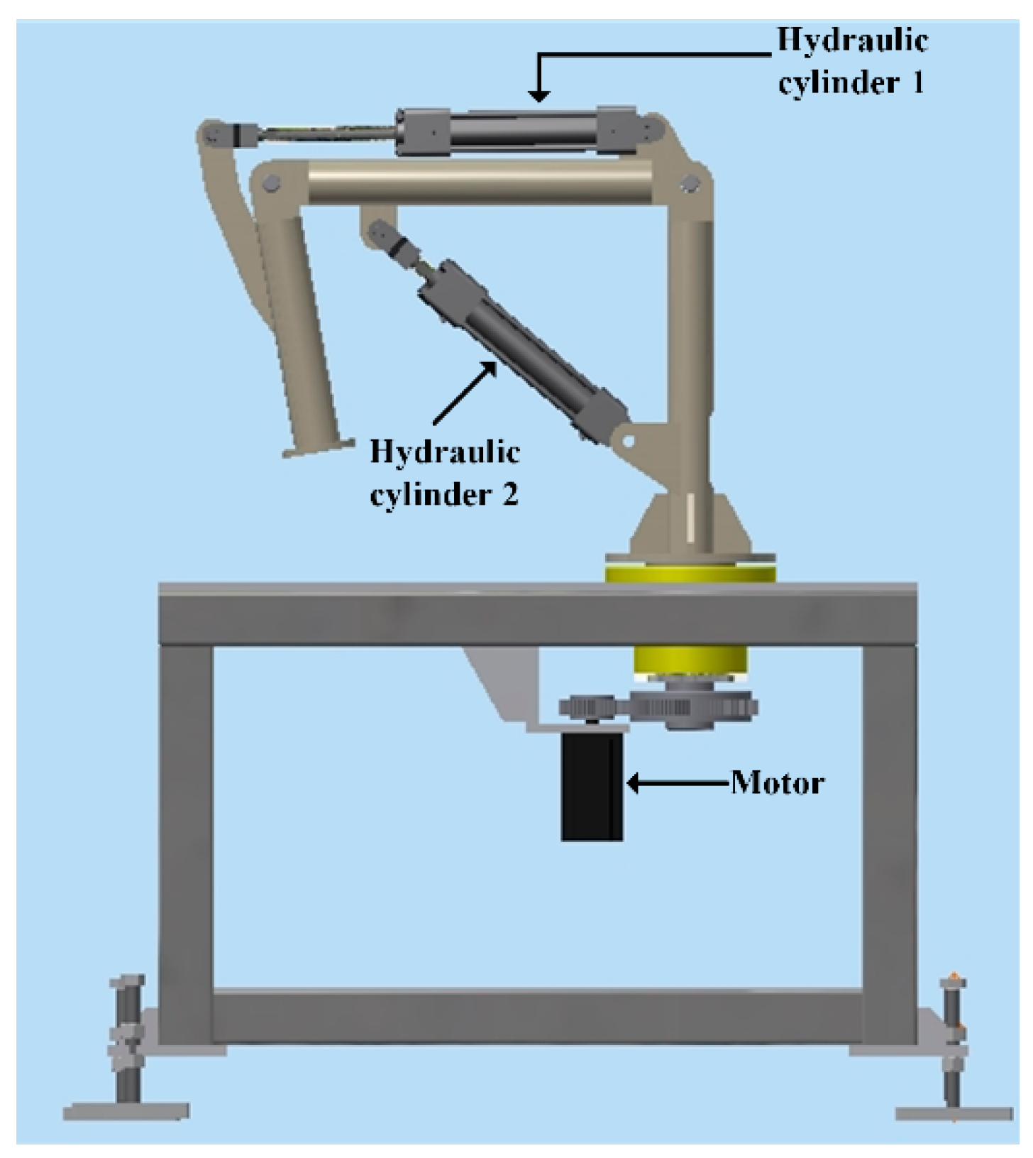
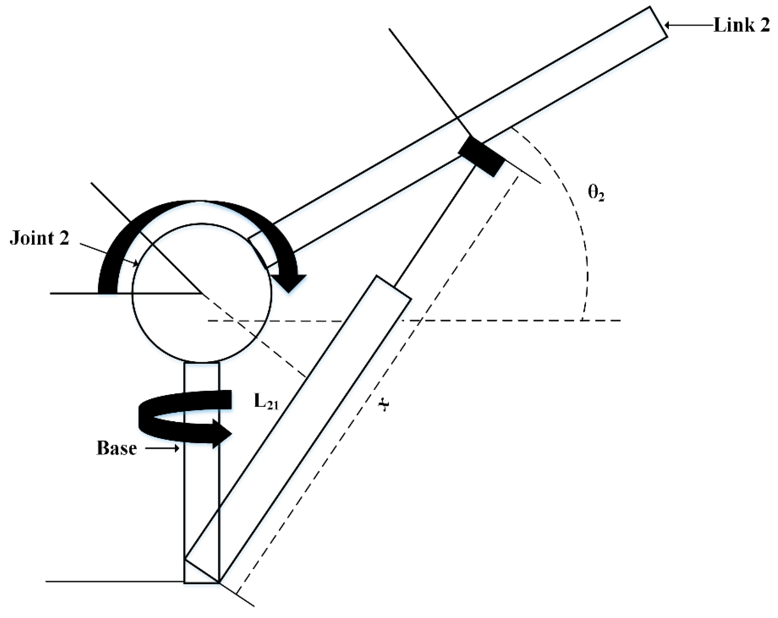
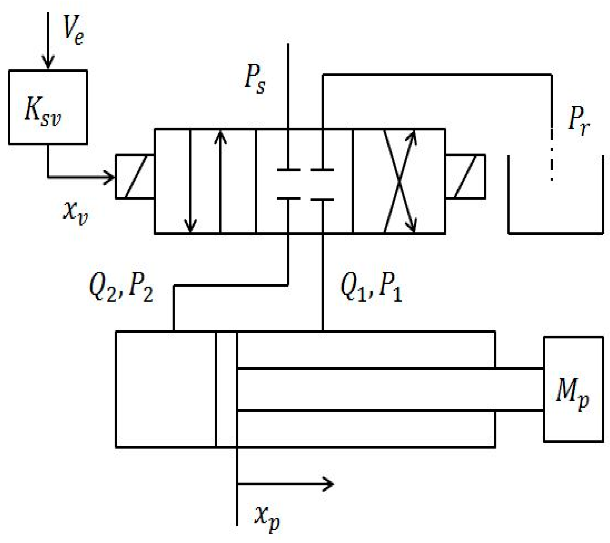
2. Mechanical Design and Dynamics of Hydraulic Servo System

It is a well-known fact that hydraulic servo systems have a favorable position in applications involving the machine tool industry. Some popular examples include handling hazardous material, remote equipment, steel factories, mining of materials, the exploration of oil, and the testing of automotive equipment, etc. A servo system is responsible, according to design, to control dynamical properties, such as; force, pressure, acceleration, electrical properties, etc. The attractive features of hydraulic servo systems include efficient response time, high torque and very few stroke characteristics. The hydraulic system has several advantages, but most prominent are accurate tracking of localization and acceleration, better stiffness features, null backlash, efficient response to sudden change, and less wear rate, among others. The hydraulic system has a better position among robotic systems to dismantle nuclear plants or hazardous plants. The hydraulic system, while used in nuclear plants, could be divided into two major parts, the first consists of a couple of hydraulic cylinders which formulate the vertical movement and the second consists of an AC servo motor responsible for horizontal changes. Two cylinders with a hydraulic mechanism is provided in the first part as much higher torque is required in the vertical direction. The mechanical design of shape and different sizes of a hydraulic servo system utilized in nuclear power plants is shown in Figure 1 and Figure 2. The modelling of hydraulic actuator has been presented in Appendix A.

The schematic design of an end effector is displayed in Figure 3 and the schematic diagram of a hydraulic servo system’s base and secondary link is shown in Figure 4.

It is a well-known fact that a robotic system dynamic is a cross-relation between different forces, acceleration properties, and localization. Thus, the dynamical equation of a robotic manipulator in free space could be represented mathematically as,

$$T=A\left(\theta \right)\ddot{\theta }+B\left(\theta ,\dot{\theta }\right)+g\left(\theta \right)$$

(1)

where $\theta$, $A\left(\theta \right),B\left(\theta ,\dot{\theta }\right),g\left(\theta \right)$ and $T$ are the vectors representing joints of angles, the matrix representing mass or inertia, the centrifugal/Coriolis torque, the gravity torque in joint space, and the vector of joint torques, respectively. Similarly, the equation repressing dynamical properties of different links in a hydraulic servo system could be represented as

$$(J_{s1}+\Delta J_{s1}){\ddot{\theta }}_1+(D_{s1}+\Delta D_{s1}+{\beta }_1){\dot{\theta }}_1+0.5M_{s1}{L}_{1}g\sin {\theta }_1+{\tau }_{e1}=T_1$$

(2)

$$(J_{s2}+\Delta J_{s2}){\ddot{\theta }}_2+(D_{s2}+\Delta D_{s2}){\dot{\theta }}_2+M_{s2}{L}_{2}g\cos {\theta }_2+{\beta }_2\dot{x}+{\tau }_{e2}+\lambda =T_2$$

(3)

$$(J_{s3}+\Delta J_{s3}){\ddot{\theta }}_3+(D_{s3}+\Delta D_{s3}){\dot{\theta }}_3+0.5M_{s3}{L}_{3}g\sin {\theta }_3+{\tau }_{e3}=T_3$$

(4)

where $J_{s1}$, $J_{s2}$ and $J_{s3}$ represent the inertia of the base, second link, and end effector respectively, similarly $D_{s1}$, $D_{s2}$ and $D_{s3}$ represents the damping characteristics of the base, second link, and end effector respectively. The uncertainty is represented by $\Delta$, ${\beta }_1$, and ${\beta }_2$ shows the viscosity of each cylinder in the first part. $M_{s1}$, $M_{s2}$ and $M_{s3}$ represent the masses of the base, second link and end effector, $L_1$ and $L_3$ are lengths of base and end effector, $L_2$ represents the length from joint to the centre of mass (COM) of the second link. ${\tau }_{e1}$, ${\tau }_{e2}$ and ${\tau }_{e3}$ represent the reaction torque generated by contact with the environment and joints 1, 2 and 3 respectively, $\lambda$ represents the dynamical properties regarding the base, ${\dot{\theta }}_1$ is the velocity of the first cylinder and $\dot{x}$ is the velocity of the second cylinder, and $T_1$, $T_2$ and $T_3$ represent joint torques of the base, second link and end effector respectively.

3. Sliding Mode Control with Sliding Perturbation Observer (SMCSPO)

3.1. Sliding Mode Control

Several previous studies have shown that the implementation of a sliding perturbation observer (SPO) and a sliding mode control (SMC) at the same time provides certain attractive features which include efficient performance against perturbation by utilizing partial state feedback. The combination of these two with such attractive properties is known as sliding mode control with sliding perturbation observer [37]. In our previous work [38], we only estimated the reaction force of the slave at the end effector. In this study, three-link robotic manipulator actuators are controlled by implementing SMC, and the reaction force is determined by applying SPO. A generic mathematical representation of n-degrees of freedom system inheriting second order dynamics is as follow,

$${\ddot{x}}_j=f_j\left(x\right)+\Delta f_j\left(x\right)+{\displaystyle \sum _{i=1}^n[(b_{ji}\left(x\right)}+\Delta b_{ji}\left(x\right))u_i]+d_j\left(t\right), j= 1, \dots ,n$$

(5)

where $x\stackrel{\Delta }{=}{[X_1\dots X_n]}^T$ represents the state vector with $X_j\stackrel{\Delta }{=}{[x_j,{\dot{x}}_j]}^T$, the non-linear driving force is represented by $f_j\left(x\right)$ with uncertainties $\Delta f_j\left(x\right)$, the elements of the control gain matrix is represented by $b_{ji}$ with corresponding uncertainties $\Delta b_{ji}$, the external disturbance and control input is represented by $d_j$ and $u_j$; respectively, and $f_j$, $b_{ji}$ are well known continuous functions of state in literature [39]. All of the uncertainties could be summed up, to represent perturbation as follow,

$${\psi }_j\left(x,t\right)=\Delta f_j\left(x\right)+{\displaystyle \sum _{i=1}^n[}\Delta b_{ji}\left(x\right)u_i]+d_j\left(t\right)$$

(6)

The objective of control is to force state x to a desired state $x_d\stackrel{\Delta }{=}{[X_{1d}\dots X_{nd}]}^T$ in the presence of perturbation. The upper bound for perturbation is defined by a known continuous function of state as follows

$${\mathsf{\Gamma }}_j\left(x,t\right)=F_j\left(x\right)+\underset{i=1}{\overset{n}{\mathsf{\Sigma }\left|{\mathsf{\Phi }}_{ji}\left(x\right)u_i\right|}}+D_j\left(t\right)>\left|{\mathsf{\Psi }}_j\left(t\right)\right|$$

(7)

where $F_j>\left|\Delta f_j\right|$, ${\mathsf{\Phi }}_{ji}>\left|\Delta b_{ji}\right|$ and $D_j>\left|d_j\right|$ represent the expected upper bounds of the uncertainties. Let us suppose $f_j\left(x\right)$, defined in Equation (5), except perturbation of Equation (6) is represented as

$$f_j\left(\widehat{x}\right)+{\displaystyle \sum _{i=1}^n{b}_{ji}\left(\widehat{x}\right)}{u}_i={\alpha }_{3j}{\overline{u}}_j$$

(8)

where ${\alpha }_{3j}$ is an arbitrary positive number, and ${\overline{u}}_j$ is the new control variable. The equations of SPO are derived as [39].

$${\dot{\widehat{x}}}_{1j}={\widehat{x}}_{2j}-k_{1j}sat({\tilde{x}}_{1j})$$

(9)

$${\dot{\widehat{x}}}_{2j}={\alpha }_3{\overline{u}}_j-k_{2j}sat({\tilde{x}}_{1j})+{\widehat{\mathsf{\Psi }}}_j$$

(10)

$${\dot{\widehat{x}}}_{3j}={\alpha }_{3j}^2\left({\overline{u}}_j+{\alpha }_{3j}{\widehat{x}}_{2j}-{\widehat{x}}_{3j}\right)$$

(11)

$${\widehat{\psi }}_j={\alpha }_{3j}({\alpha }_3{\widehat{x}}_{2j}-{\widehat{x}}_{3j})$$

(12)

where $k_{1j}$, $k_{2j}$, ${\alpha }_{3j}$ are positive numbers and $\tilde{x}=\widehat{x}-x$ is the estimation error of the measurable state. ${\widehat{\psi }}_j$ is defined as the estimated perturbation of the robot manipulator. The “˜” and “^” represent the error in estimation and quantity estimated in result of the estimation respectively.

$$sat({\tilde{x}}_{1j})=\{\begin{array}{cc}{\tilde{x}}_{1j}/\left|{\tilde{x}}_{1j}\right|,\hfill & if\left|{\tilde{x}}_{1j}\right|\ge {\epsilon }_{0j}\hfill \\ {{\tilde{x}}_{1j}/\epsilon }_{0j},\hfill & if\left|{\tilde{x}}_{1j}\right|\le {\epsilon }_{0j}\hfill \end{array}$$

(13)

The anti-chatter properties are formulated by a saturation function defined by Slotine et al. [40] where the boundary layer of SMC control is represented by ${\epsilon }_{0j}$. Finally, the error dynamics of SPO are mathematically defined as [39],

$${\dot{\tilde{x}}}_{1j}={\tilde{x}}_{2j}-k_{1j}sat({\tilde{x}}_{1j})$$

(14)

$${\dot{\tilde{x}}}_{2j}=-k_{2j}sat({\tilde{x}}_{1j})+{\tilde{\mathsf{\Psi }}}_j$$

(15)

$${\dot{\tilde{x}}}_{3j}=-{\alpha }_{3j}^2\left({\alpha }_{3j}{\tilde{x}}_{2j}-{\tilde{x}}_{3j}\right)+\dot{\mathsf{\Psi }}/{\alpha }_{3j}$$

(16)

After the observer sliding mode begins, ${\tilde{x}}_{2j}$ dynamics become

$${\dot{\tilde{x}}}_{2j}+\left(k_{2j}/k_{1j}\right){\tilde{x}}_{2j}={\tilde{\mathsf{\Psi }}}_j$$

(17)

The frequency domain relation between ${\tilde{\mathsf{\Psi }}}_j$ and ${\mathsf{\Psi }}_j$ is derived as

$${\tilde{\mathsf{\Psi }}}_j\left(p\right)=\frac{p\left[p^2+\left(k_{1j}/{\epsilon }_{0j}\right)p+k_{2j}/{\epsilon }_{0j}\right]}{p^3+\left(k_{1j}/{\epsilon }_{0j}\right)p^2+\left(k_{1j}/{\epsilon }_{0j}\right)p+{\alpha }_{3j}^2\left(k_{2j}/{\epsilon }_{0j}\right)}\left(-{\mathsf{\Psi }}_j\left(p\right)\right)$$

(18)

and this is equivalent to a high-pass filter. The sliding function is defined as

$$s_j={\dot{e}}_j+c_{1j}{e}_j$$

(19)

where $e_j=x_{1j}-x_{1dj}$ is the actual position tracking error, $c_{1j}>0$. As the sliding surface is reached, we define ${\dot{s}}_j=0$ and sliding control is defined as

$${\dot{s}}_j=-K_{j}sat(s_j)$$

(20)

where robust gain is represented by $K_j$ and is supposed to be positive. The control input $u_j$ is mathematically defined as follows,

$$u_j=B^{-1}Col{({\ddot{x}}_{1dj}+f_j(x)+c{\dot{e}}_j)}_j-K_{j}sat(s_j)$$

(21)

Similarly, the estimated sliding function is represented mathematically as

$${\widehat{s}}_j={\dot{\widehat{e}}}_j+c_{j1}{\widehat{e}}_j$$

(22)

where, the estimation error of localizing tracking is ${\widehat{e}}_j={\widehat{x}}_{1j}-x_{1dj}$ and jth degree of freedom motion ${[x_{1dj}{\dot{x}}_{1dj}]}^T$ and $c_{j1}>0$. Similarly, the estimation error in sliding function is mathematically represented by ${\tilde{s}}_j={\widehat{s}}_j-s_j$. The estimation error in sliding function can be calculated by using Equations (19) and (22) as

$${\tilde{s}}_j={\dot{\tilde{x}}}_{1j}+c_{j1}{\tilde{x}}_{1j}$$

(23)

The new control input ${\overline{u}}_j$ is designed such that it forces $\dot{\widehat{s}}\widehat{s}<0$ outside of the prescribed manifold. The desired ${\widehat{s}}_j$-dynamics is defined as

$${\dot{\widehat{s}}}_j=-K_{j}sat({\widehat{s}}_j)$$

(24)

Thus ${\dot{\widehat{s}}}_j$ can be calculated as follows

$$\begin{array}{l}{\dot{\widehat{s}}}_j={\alpha }_{3j}{\overline{u}}_j-\left[k_{2j}/{\epsilon }_{0j}+c_{j1}\left(k_{1j}/{\epsilon }_{0j}\right)-{\left(k_{1j}/{\epsilon }_{0j}\right)}^2\right]{\tilde{x}}_{1j}\\ -\left(k_{1j}/{\epsilon }_{0j}\right){\tilde{x}}_{2j}-{\ddot{x}}_{1jd}+c_{j1}\left({\widehat{x}}_{2j}-{\dot{x}}_{1jd}\right)+{\widehat{\psi }}_j\end{array}$$

(25)

The control law to apply Equation (23) with ${\tilde{x}}_{2j}=0$ is defined as

$$\begin{array}{l}{\overline{u}}_j=\frac{1}{{\alpha }_{3j}}\{-K_{j}sat({\widehat{s}}_j)+[\frac{k_{2j}}{{\epsilon }_{0j}}+c_{j1}\frac{k_{1j}}{{\epsilon }_{0j}}-{(\frac{k_{1j}}{{\epsilon }_{0j}})}^2]{\tilde{x}}_{1j}\\ +{\ddot{x}}_{1jd}-c_{j1}({\widehat{x}}_{2j}-{\dot{x}}_{1jd})-{\widehat{\psi }}_j\}\end{array}$$

(26)

where ${\overline{u}}_j$ represents the control input of SMCSPO. Thus, the resulting ${\widehat{s}}_j$-dynamics including the effects of ${\tilde{x}}_{2j}$ could be mathematically represented as

$${\dot{\widehat{s}}}_j=-K_{j}sat({\widehat{s}}_j)-\left(k_{1j}/{\epsilon }_{0j}\right){\tilde{x}}_{2j}$$

(27)

To ensure the outer part of the manifold $\left|{\widehat{s}}_j\right|\le {\epsilon }_{0j}$ satisfies the inequality $\dot{\widehat{s}}\widehat{s}<0$, the robust control gain must be constrained to the following inequality

$$K_j\ge k_{1j}^2/{\epsilon }_{0j}$$

(28)

Finally, the actual $s_j$-dynamics within the boundary layer of $\left|{\widehat{s}}_j\right|\le {\epsilon }_{0j}$ can be mathematically expressed as

$$\begin{array}{l}{\dot{s}}_j+\frac{K_j}{{\epsilon }_{0j}}{s}_j=\left[\frac{k_{2j}}{{\epsilon }_{0j}}-\left(\frac{k_{1j}}{{\epsilon }_{0j}}-\frac{K_j}{{\epsilon }_{0j}}\right)\left(c_{j1}-\frac{k_{1j}}{{\epsilon }_{0j}}\right)\right]{\tilde{x}}_{1j}\\ -\left(c_{j1}+\frac{K_j}{{\epsilon }_{0j}}\right){\tilde{x}}_{2j}-{\tilde{\psi }}_j\end{array}$$

(29)

The estimation errors in state estimation and perturbation are the driving force for $s_j$-dynamics. The target of the designed SMCSPO is to minimize mismatch b/w the actual and desired trajectory. The sliding perturbation observer is responsible for reducing the estimation error ${\tilde{x}}_j$ in the observer part. Therefore, the sliding mode control is designed for error ${\widehat{e}}_j$ reduction b/w desired and actual values of the trajectory. Thus, implementation of SMC and SPO simultaneously guarantee the accurate results of trajectory tracking with a reduction of error.

The mechanical hardware limitations restrict the design procedure as described in Jairo et al. [39]. The instant when $\left|{\widehat{s}}_j\right|\le {\epsilon }_{0j}$, the observer design and $s_j$-dynamics, can be represented in mathematical form as below,

$$\left[\begin{array}{c}{\dot{\tilde{x}}}_{1j}\\ {\dot{\tilde{x}}}_{2j}\\ {\dot{\tilde{x}}}_{3j}\\ {\dot{s}}_j\end{array}\right]=\left[\begin{array}{cccc}-k_{1j}/{\epsilon }_{0j}& 1& 0& 0\\ -\raisebox{1ex}{$k_{2j}$}\!\left/ \!\raisebox{-1ex}{${\epsilon }_{0j}$}\right.& {\alpha }^2{}_{3j}& -{\alpha }_{3j}& 0\\ 0& {\alpha }^3{}_{3j}& -{\alpha }^2{}_{3j}& 0\\ k_{2j}/{\epsilon }_{0j}-{\left(c-k_{1j}/{\epsilon }_{0j}\right)}^2& -\left(2c+{\alpha }^2{}_{3j}\right)& {\alpha }_{3j}& -c\end{array}\right]\cdot \left[\begin{array}{c}{\tilde{x}}_{1j}\\ {\tilde{x}}_{2j}\\ {\tilde{x}}_{3j}\\ s_j\end{array}\right]+\left[\begin{array}{c}0\\ 0\\ 1\\ 0\end{array}\right]{\dot{\psi }}_j/{\alpha }_{3j}$$

(30)

where a square matrix of order 4 in Equation (30) represents the state matrix. Further suppose, $\lambda$ represents the eigen values of state matrix A, then its characteristic equation det $\left|\lambda I-A\right|=0$, can be expressed as,

$$\left[\lambda +c_{j1}\right]\left[{\lambda }^3+\left(k_{1j}/{\epsilon }_{0j}\right){\lambda }^2+\left(k_{2j}/{\epsilon }_{0j}\right)\lambda +{\alpha }^2{}_{3j}\left(k_{2j}/{\epsilon }_{0j}\right)\right]=0$$

(31)

By implementing the pole-placement method, let us introduce a desired characteristic polynomial $p\left({\lambda }_d\right)={\left(\lambda +{\lambda }_d\right)}^4$ which leads to a design solution

$$\begin{gathered} k_{1j}/{\epsilon }_{0j}=3{\lambda }_d \\ {k}_{2j}/k_{1j}={\lambda }_d \\ {\alpha }_{3j}=\sqrt{{\lambda }_d/3} \\ c=K_j/{\epsilon }_{0j}={\lambda }_d \end{gathered}$$

(32)

It is obvious that a reduction in error and an increase in the accuracy of observations could be achieved with a large value of gain ${\lambda }_d$. But Jairo et al. [41] has categorically shown the limitation of breakpoints of sliding function dynamics encircled in a manifold. They showed that it could not go beyond $1/5{\tau }^{hw}$, where $h$ is a positive number, and frequency is represented by $w$. Another study by Slotine et al. [42] also showed the same results. Thus, the optimal gain value could be selected as

$${\lambda }_d=\frac{1}{15{\tau }^{hw}}$$

(33)

3.2. Reaction Force Estimation Based upon Sliding Perturbation Observer (SPO)

The algorithm using SPO could be utilized to set an estimate of perturbation that leads to the determination of reaction force. The perturbation’s estimation includes two factors, the first disturbance that is regarded as an external force and another is the dynamic error that inherits non-linear terms and viscous friction. The 3DOF robotic-manipulator defined in Equations (2) and (3) can be used to define a perturbation estimate that would be used to determine the reaction force. The perturbation estimate of the end-effector and second link are mathematically represented by an expression defined below,

$${\widehat{\psi }}_{s1}=-\frac{1}{J_{s1}}({\widehat{\tau }}_{e1})-\frac{1}{J_{s1}}(0.5M_{s1}{L}_{1}g\sin {\theta }_1)-(\frac{\Delta J_{s1}}{J_{s1}}){\ddot{\theta }}_1-\frac{1}{J_{s1}}(\Delta B_{s1}+{\beta }_1){\dot{\theta }}_1$$

(34)

$${\widehat{\psi }}_{s2}=-\frac{1}{J_{s2}}({\widehat{\tau }}_{e2})-\frac{1}{J_{s2}}(M_{s2}{L}_{2}g\cos {\theta }_2)-(\frac{\Delta J_{s2}}{J_{s2}}){\ddot{\theta }}_1-\frac{1}{J_{s2}}(\Delta B_{s2}{\dot{\theta }}_2)-\frac{1}{J_{s2}}({\beta }_2\dot{x})-\frac{1}{J_{s2}}(\lambda )$$

(35)

The Equations (34) and (35) further used to calculate the reaction force as follows

$${\widehat{\tau }}_{e1}=J_{s1}{\widehat{\psi }}_{s1}+0.5M_{s1}{L}_{1}g\sin {\theta }_1+\Delta J_{s1}{\ddot{\theta }}_1+(\Delta B_{s1}+{\beta }_1){\dot{\theta }}_1$$

(36)

$${\widehat{\tau }}_{e2}=J_{s2}{\widehat{\psi }}_{s2}+M_{s2}{L}_{2}g\cos {\theta }_2+\Delta J_{s2}{\ddot{\theta }}_1+\Delta B_{s2}{\dot{\theta }}_2+{\beta }_2\dot{x}+\lambda$$

(37)

where ${\widehat{\tau }}_{e1}$, ${\widehat{\tau }}_{e2}$ are the estimates of reaction torques generated as a result of contact with the environment of the end-effector and second link respectively, $\Delta$ represents the uncertainty parameter. It is worthy to mention that if the parameter is well estimated than the parameter of uncertainty could be considered as well.

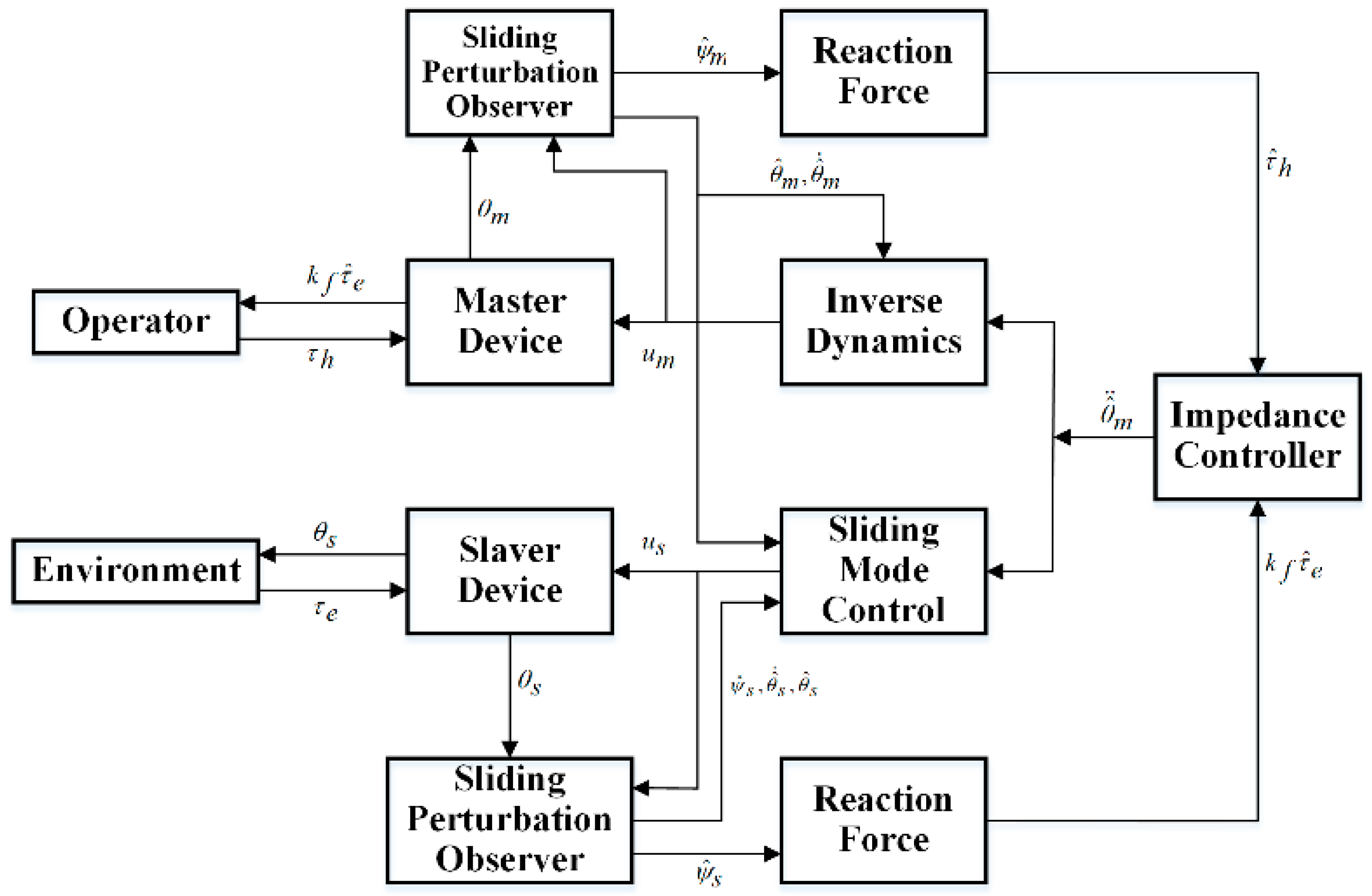
4. Bilateral Control Design between Master and Slave for 3DOF Hydraulic Servo System

4.1. Bilateral Control

The design purpose of bilateral control refers to a relation b/w the master and slave system helping the system operator in a way that is as close as the actual environment. There are two important factors that need to be considered while designing bilateral control. The first is that the slave accurately follows the trajectory of the master system and the second that the system’s operator gets a realistic feel of a reaction force. In this study, the master and slave system are 3DOF hydraulic servo systems. The dynamical equations for these two systems are shown in Equations (38) and (39).

$$J_m{\ddot{\theta }}_m+B_m{\dot{\theta }}_m=u_m+{\tau }_h$$

(38)

$$J_s{\ddot{\theta }}_s+B_s{\dot{\theta }}_s=u_s-{\tau }_e$$

(39)

where $J_m$, $J_s$, $u_m$ and $u_s$ are inertia, position, and control input of master and slave of hydraulic servo system respectively. ${\tau }_h$ represents the real/action force generated by the operator at the master device, ${\tau }_e$ defines the reaction force of the slave system in a remote environment. A detailed workflow of the control algorithm for bilateral control is presented in Figure 5.

A simple fact is that as the master device is operated by a human operator, the slave system follows the trajectory of the master system. The slave system of hydraulic servos follows the master’s trajectory using a sliding mode control. The impedance control is implemented to transfer reaction force during trajectory tracking. Therefore, no reaction force is observed by the operator while there are no contact between the slave and environment.

4.2. Master Controller and Device

The design of the master system has been considered under two constraints. The first one is that the reaction force is felt by the operator during the slave system and environment contact. The second constraint is that the operator uses the master system with the minimal force possible. The design of the impedance control is defined as,

$$J_d{\ddot{\theta }}_m+B_d{\dot{\theta }}_m+K_d{\theta }_m={\widehat{\tau }}_h-k_f{\widehat{\tau }}_e$$

(40)

where $J_d$, $B_d$ and $K_d$ are the inertia, damping, and stiffness of the impedance control model respectively, $k_f$ represents the scale factor of the reaction force. The scale factor $k_f$ scales the force ratio that is converted from the master system to the slave system. For simplicity, in this study $k_f$ is considered to be unity. The control input signal to the master system can be determined by replacing the estimated/observed state variable to the original ones. Thus, the control input for a dynamical system of Equation (38) and impedance control of Equation (40) can be mathematically presented as follows,

$$u_m=(B_m-\frac{J_m}{J_d}{B}_d){\dot{\widehat{\theta }}}_m+(\frac{J_m}{J_d}-1){\widehat{\tau }}_h-\frac{J_m}{J_d}(k_f{\widehat{\tau }}_e+K{\widehat{\theta }}_m)$$

(41)

where $u_m$, ${\dot{\widehat{\theta }}}_m$, ${\dot{\widehat{\theta }}}_m$ are the control input, estimated speed and estimated position of the master system by utilizing SPO, ${\widehat{\tau }}_h$ represents the torque estimate that is produced by the operator while operating the master device. The master device used in this research is presented in Figure 6.

4.3. Slave Controller and Device

The slave controller is designed to track the trajectory of the master system. The slave controller is designed by utilizing SMCSPO for this study. The logic behind the SMCSPO design is to compensate sliding mode control for the perturbation estimate. It is an additive quantity consisting of uncertainty, disturbance, and non-linearity [39]. Thus, SMCSPO design efficiently removes the external disturbance and uncertainty of parameters. The sliding function that is estimated can be expressed as

$$\widehat{s}=\dot{\widehat{e}}+c\widehat{e}$$

(42)

where $\widehat{e}={\widehat{\theta }}_{s1}-{\widehat{\theta }}_{m1}$ is the tracking error between the master and slave device, $c$ is a positive constant. By substituting the observed/estimated state in the sliding function defined above in Equation (42) and the sliding perturbation observer of Equation (12), the differential of the estimated sliding surface $\widehat{s}$ can be mathematically represented as

$$\begin{array}{l}\dot{\widehat{s}}={\alpha }_{s3}{\overline{u}}_s-\frac{k_{s2}}{{\epsilon }_{s0}}{\tilde{\theta }}_{s1}-{\alpha }_{s2}{\tilde{\theta }}_{s1}+{\widehat{\psi }}_s-\frac{k_{s1}}{{\epsilon }_{s0}}{\dot{\tilde{\theta }}}_{s1}\\ -{\alpha }_{s1}{\dot{\tilde{\theta }}}_{s1}-{\ddot{\widehat{\theta }}}_{m1}+c({\dot{\widehat{\theta }}}_{s1}-{\dot{\widehat{\theta }}}_{m1})\end{array}$$

(43)

It is found that ${\alpha }_{s1}{\dot{\tilde{\theta }}}_{s1},{\alpha }_{s2}{\tilde{\theta }}_{s1}\approx 0$ when the phase is converged to the sliding surface and error estimate ${\tilde{\theta }}_{s1}$ remains inside boundary layer. The impedance model Equations (40) and (43) are utilized to obtain $\dot{\widehat{s}}$.

$$\begin{array}{l}\dot{\widehat{s}}={\alpha }_3{\overline{u}}_s-[\frac{k_{s2}}{{\epsilon }_{s0}}+c(\frac{k_{s1}}{{\epsilon }_{s0}})-(\frac{k_{s1}}{{\epsilon }_{s0}}{{\displaystyle )}}^2]{\tilde{\theta }}_{s1}-J_d^{-1}({\widehat{\tau }}_h\\ -k_f{\widehat{\tau }}_e-B_d{\dot{\widehat{\theta }}}_m-K_d{\widehat{\theta }}_m)+{\widehat{\psi }}_s+c({\dot{\widehat{\theta }}}_{s1}-{\dot{\widehat{\theta }}}_{m1})\end{array}$$

(44)

The new control variable ${\overline{u}}_s$ is chosen under the constraint i.e., $\dot{\widehat{s}}\widehat{s}<0$. Similarly, $\dot{\widehat{s}}$ dynamics is chosen to satisfy the sliding mode condition

$$\dot{\widehat{s}}=-Ksat(\widehat{s})$$

(45)

The new control input presented in Equation (8) can be found from Equations (44) and (45)

$$\begin{array}{l}{\overline{u}}_s={\alpha }_{s3}^{-1}\{-Ksat(\widehat{s})+[\frac{k_{s2}}{{\epsilon }_{s0}}+c(\frac{k_{s1}}{{\epsilon }_{s0}})-(\frac{k_{s1}}{{\epsilon }_{s0}}{{\displaystyle )}}^2]{\tilde{\theta }}_{s1}\\ +J_d^{-1}(B_d{\dot{\widehat{\theta }}}_m+K_d{\widehat{\theta }}_m-{\widehat{\tau }}_h+k_f{\widehat{\tau }}_e)-c({\dot{\widehat{\theta }}}_{s1}-{\dot{\widehat{\theta }}}_{m1})-{\widehat{\psi }}_s\}\end{array}$$

(46)

Final control input for the slave system is mathematically defined as

$$u_s=J_s{\overline{u}}_s+B_s{\dot{\widehat{\theta }}}_s$$

(47)

5. Experimental Environment

The slave device for the experiment is shown in Figure 7. The hydraulic servo system consists of two hydraulic cylinders and one AC servo motor. The first base axis is actuated by the AC servo motor. The 2nd link and end effector are actuated by the hydraulic cylinder.

The experiments were performed on a 3DOF hydraulic servo system.

Table 1. Hydraulic servo system.

S. No	Items	Specification
1	Hydraulic cylinder	Piston and rod diameter = 0.04 m, 0.022 Stroke = 20 cm
2	Hydraulic pump	P_max = 210 bar Q_max = 20 1/min
3	Displacement transducer	Stroke = 20 cm (10 V)
4	Propositional directional control valve	D633-313A, Moog, Inc.
5	Relief valve	P_set = 20 bar
6	Control board	PC based MMC

, shows the specifications of a hydraulic servo system.

In [43,44], the identification and robust control of a hydraulic servo system have been discussed. The unknown parameters such as the inertia and damping coefficients of the system are obtained by the signal compression method which can estimate the dynamics by obtaining an equivalent impulse response [45]. The model dynamic is given by

$$\ddot{x}=\frac{1}{J_i}u-\frac{1}{J_i}{D}_i\dot{x}, i= 1, 2, 3$$

(48)

where $J_i$, $D_i$ are the equivalent moments of inertia and damper respectively.

Table 2. Hydraulic servo system dynamics parameters.

S. No	Moment of Inertia (Master) kg·m2	Moment of Inertia (Slave) kg·m2	Damper (Master) kg·m2	Damper (Slave) kg·m2
1	1.35135	303.26	3.99	17,355.5
2	1.5	59.52	3.99	5241.66
3	0.74	355.91	3.99	2214

, shows the values of the dynamics.

The experimental setup includes a master device, a slave device and a control system as shown in Figure 8.

The master and slave device consist of three links each, in which the third link is connected with the base. We can find the reaction force at end effector and the 2nd link. SMCSPO is used to estimate the reaction force. Since the operator moves the master device to make the slave come in contact with a hard object, a visual sensor is installed with the slave device. It is not relevant to the control algorithm but provides visual feedback to the operator to avoid any inconvenience or uncertain situations. Figure 9 provides a pictorial view of visual feedback which helps enhance the safety during work.

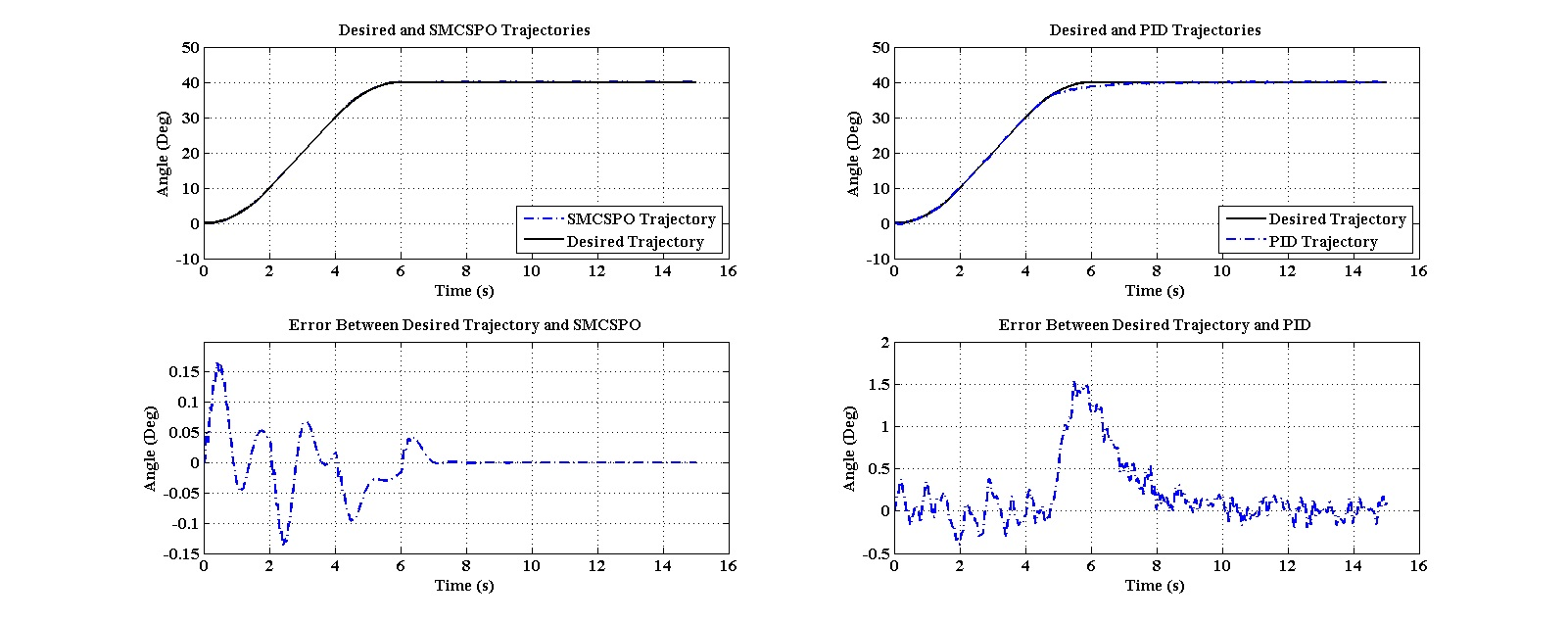
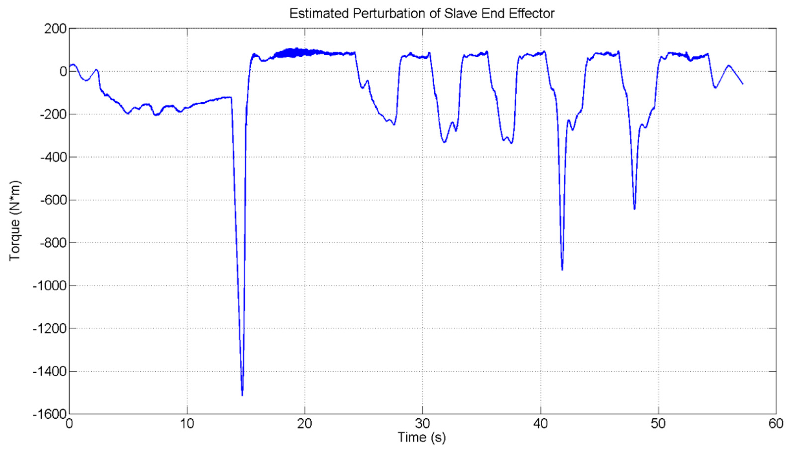
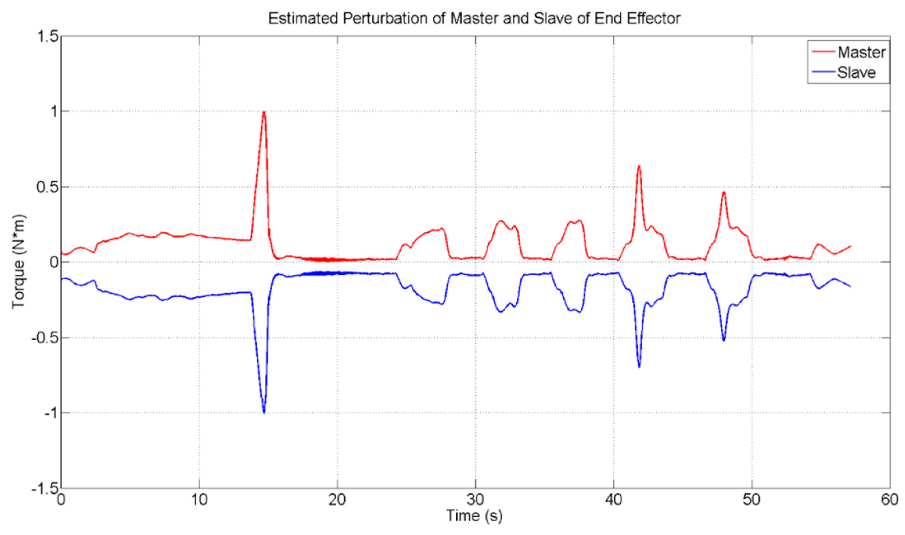
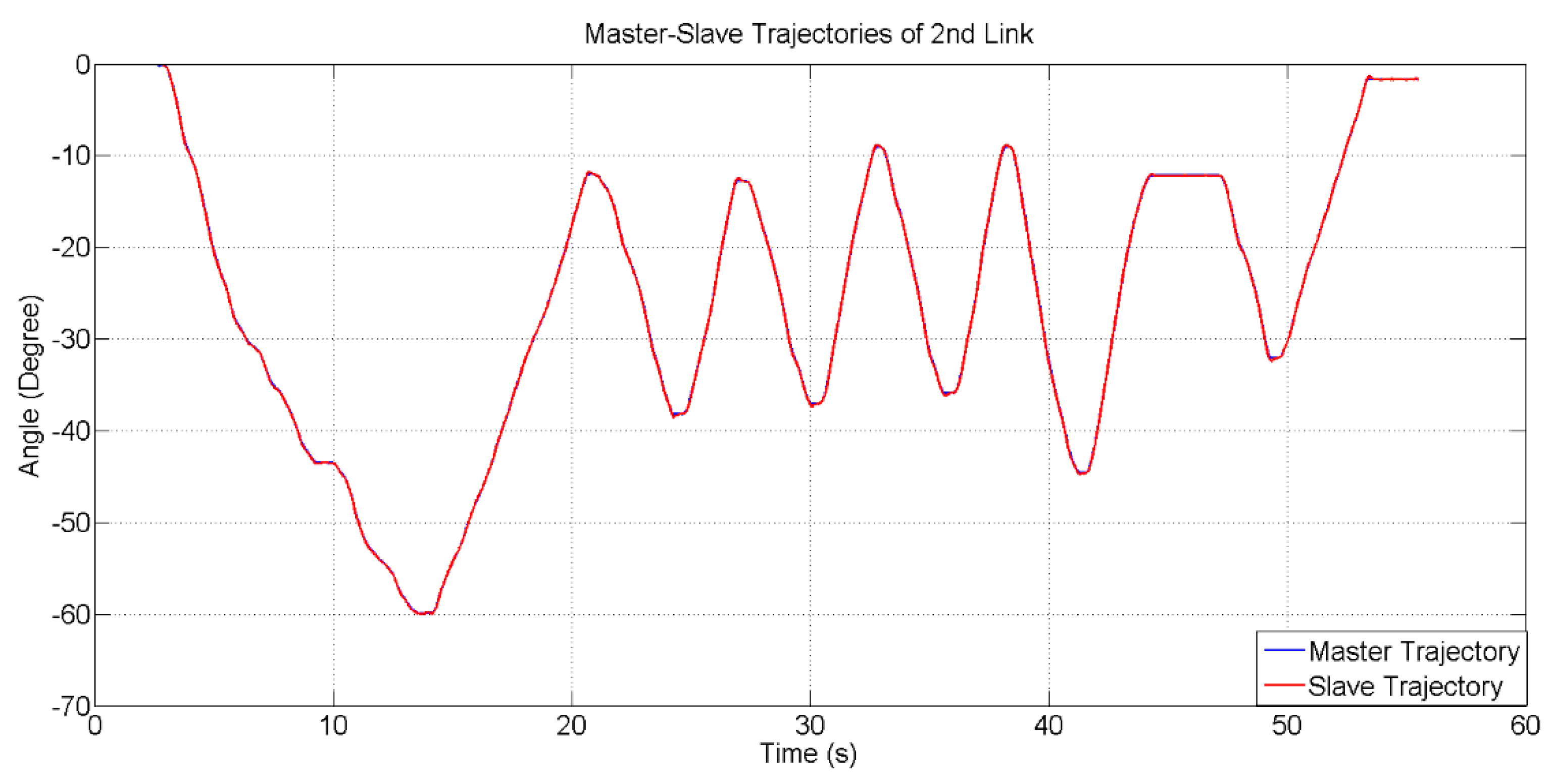
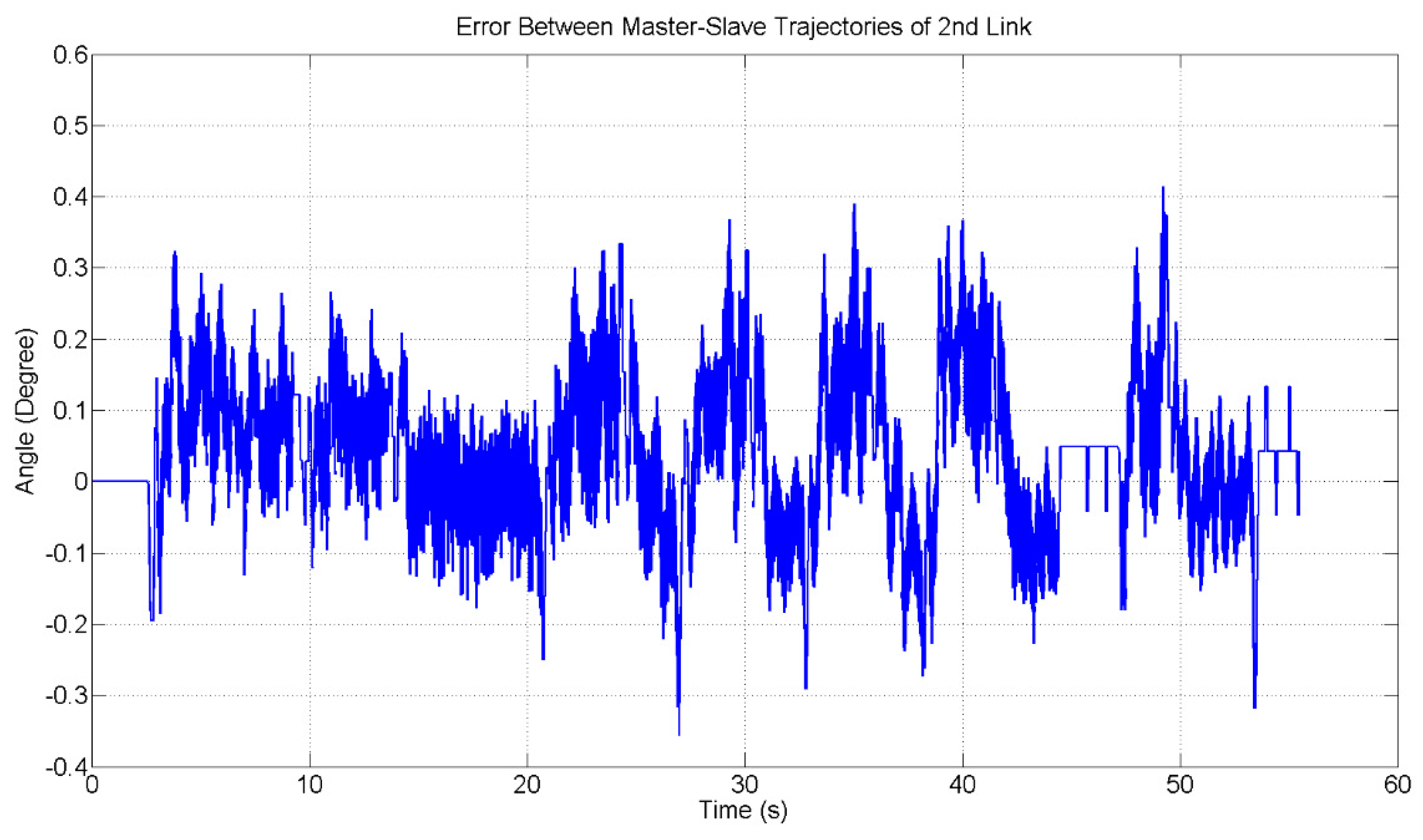
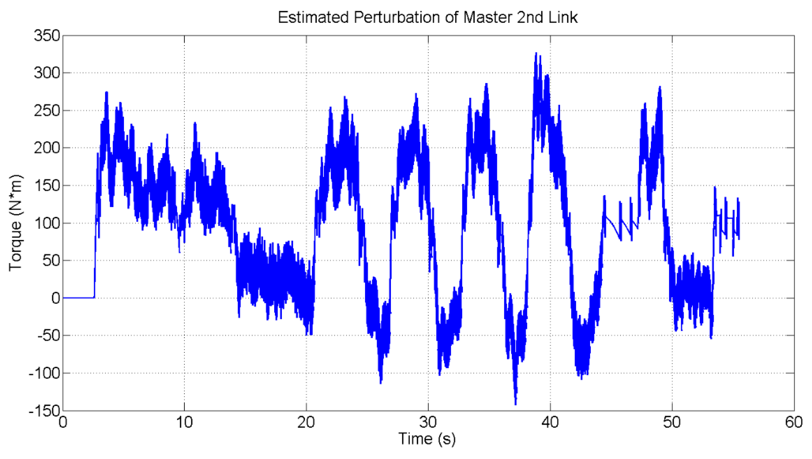
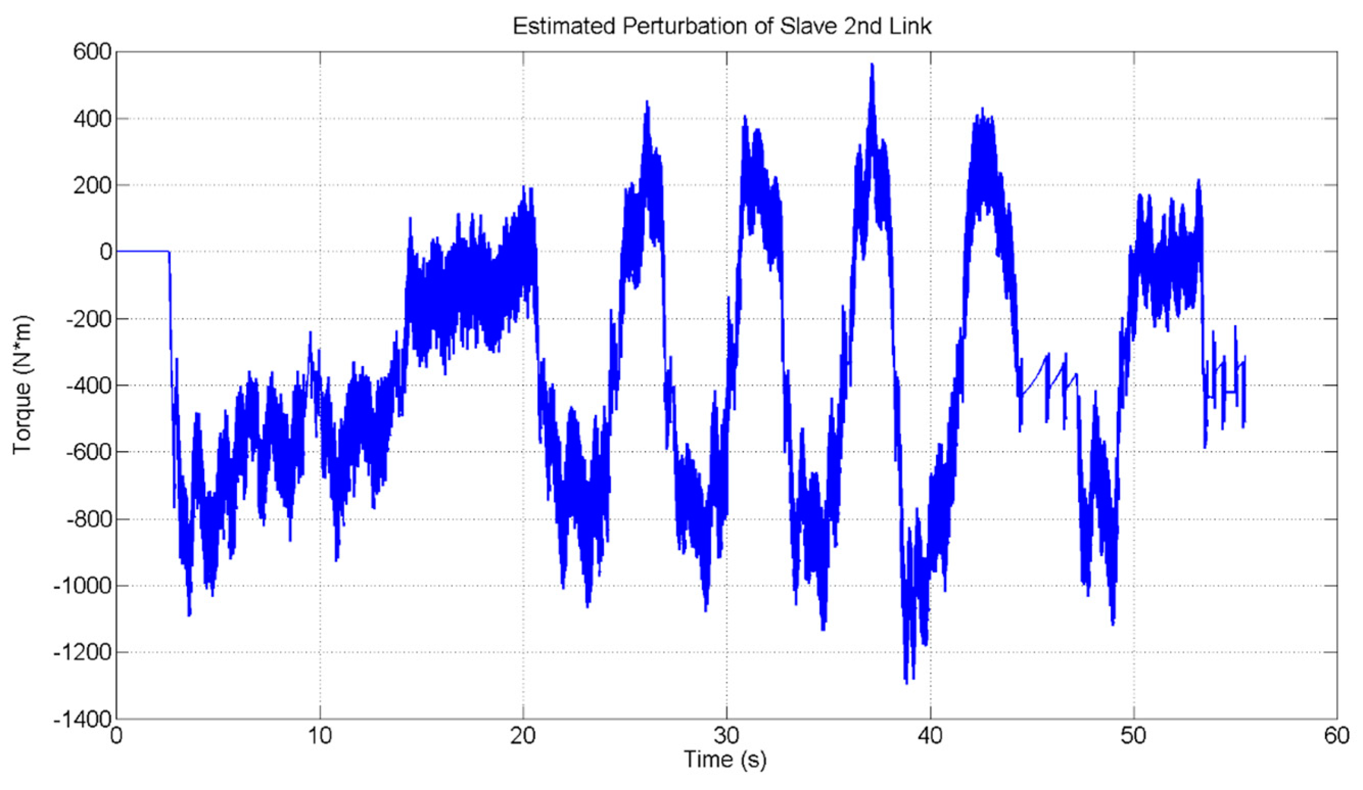
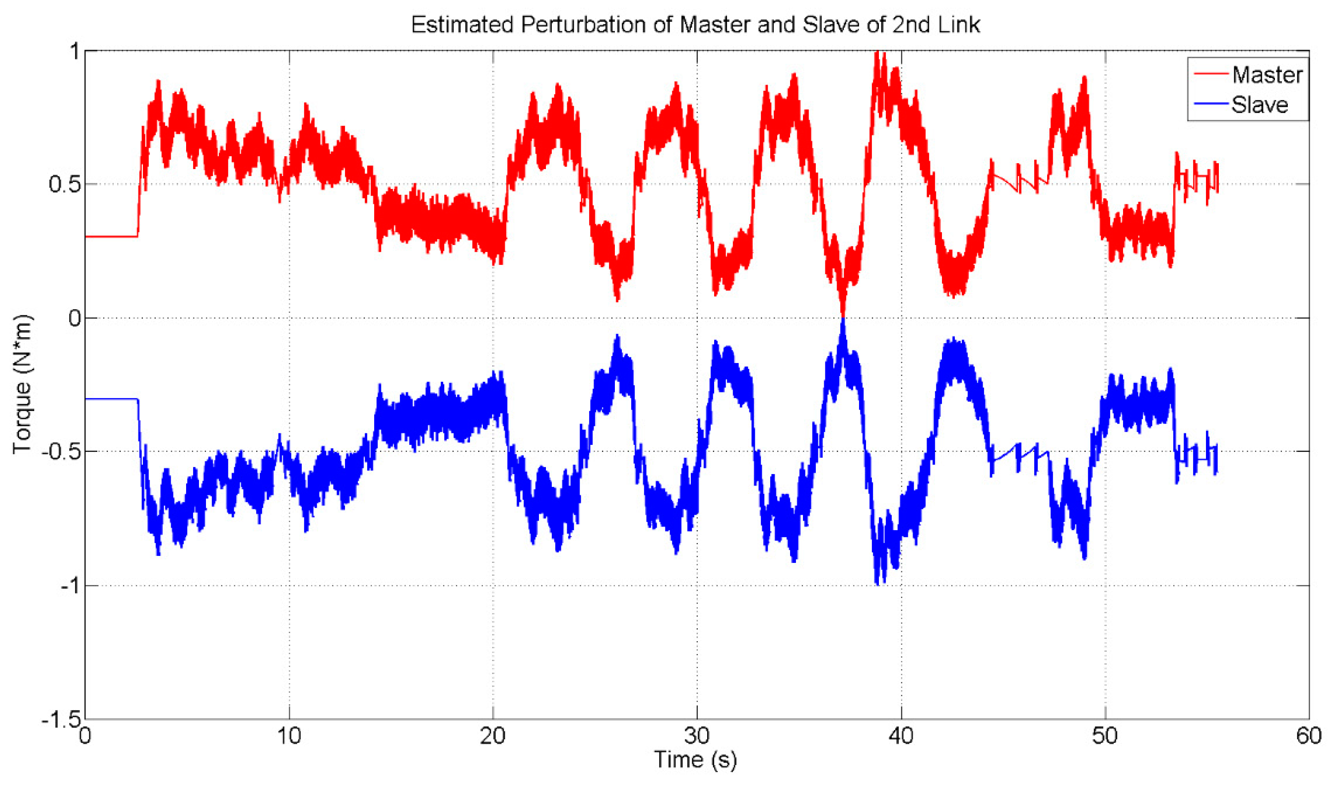
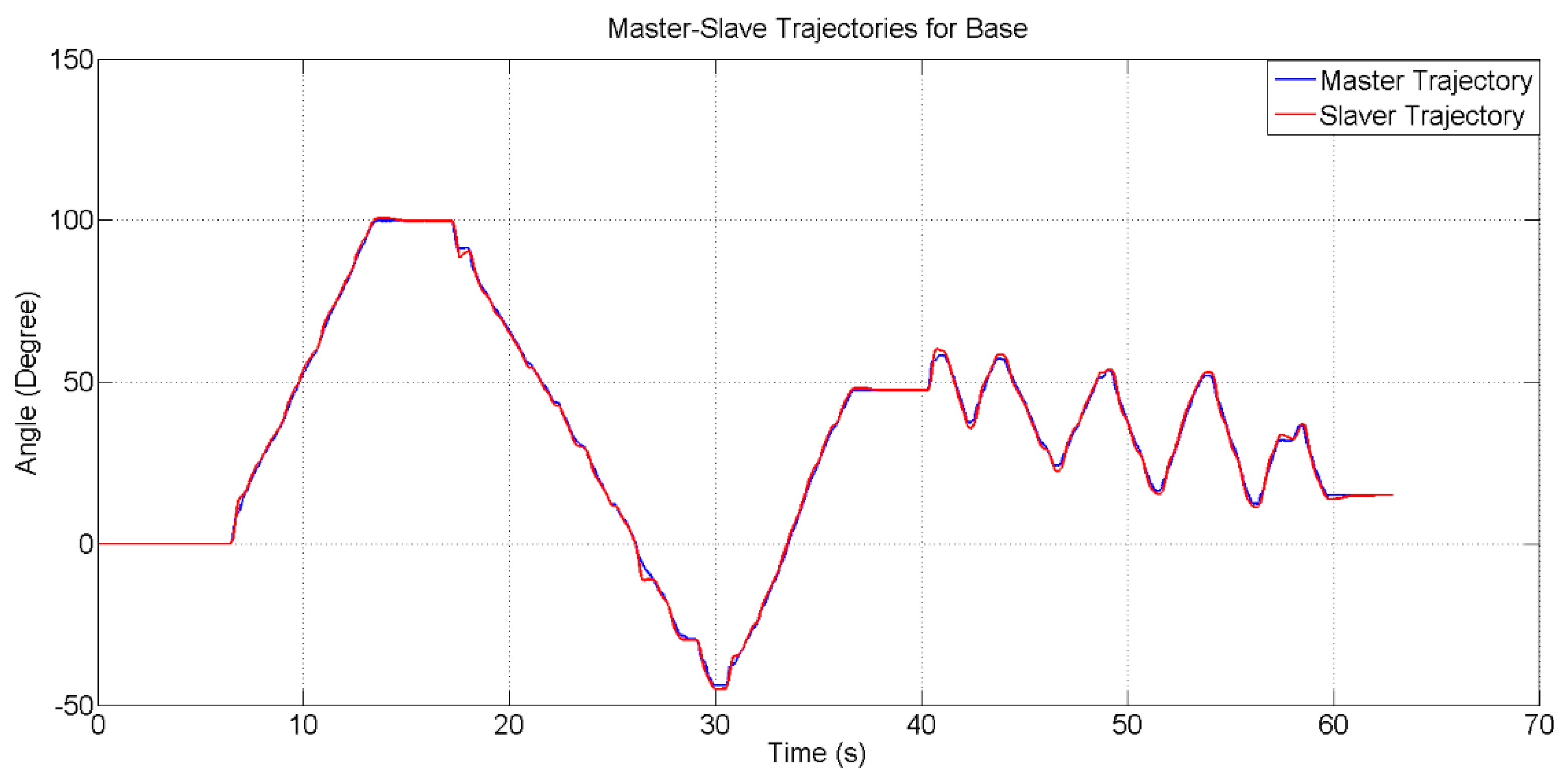
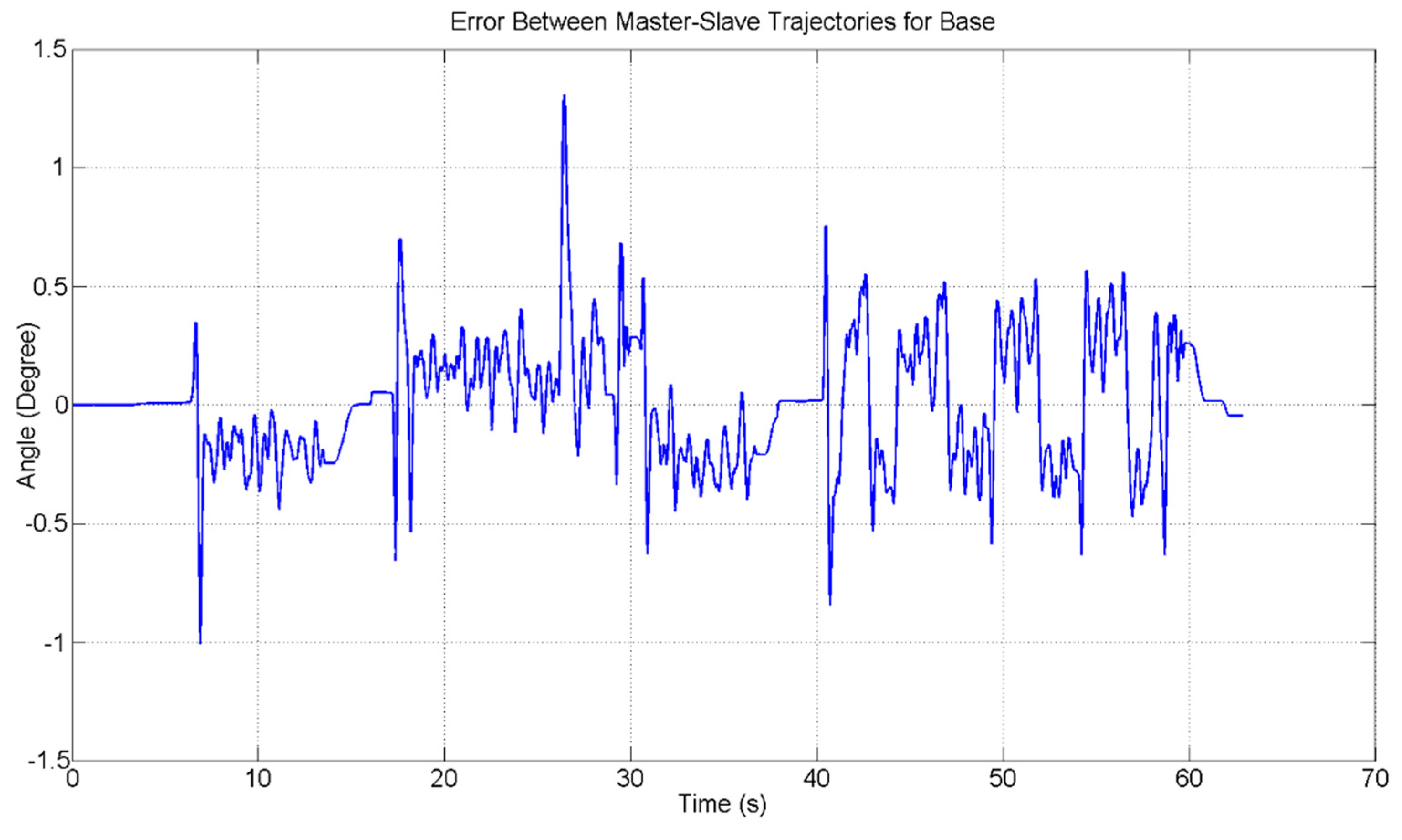
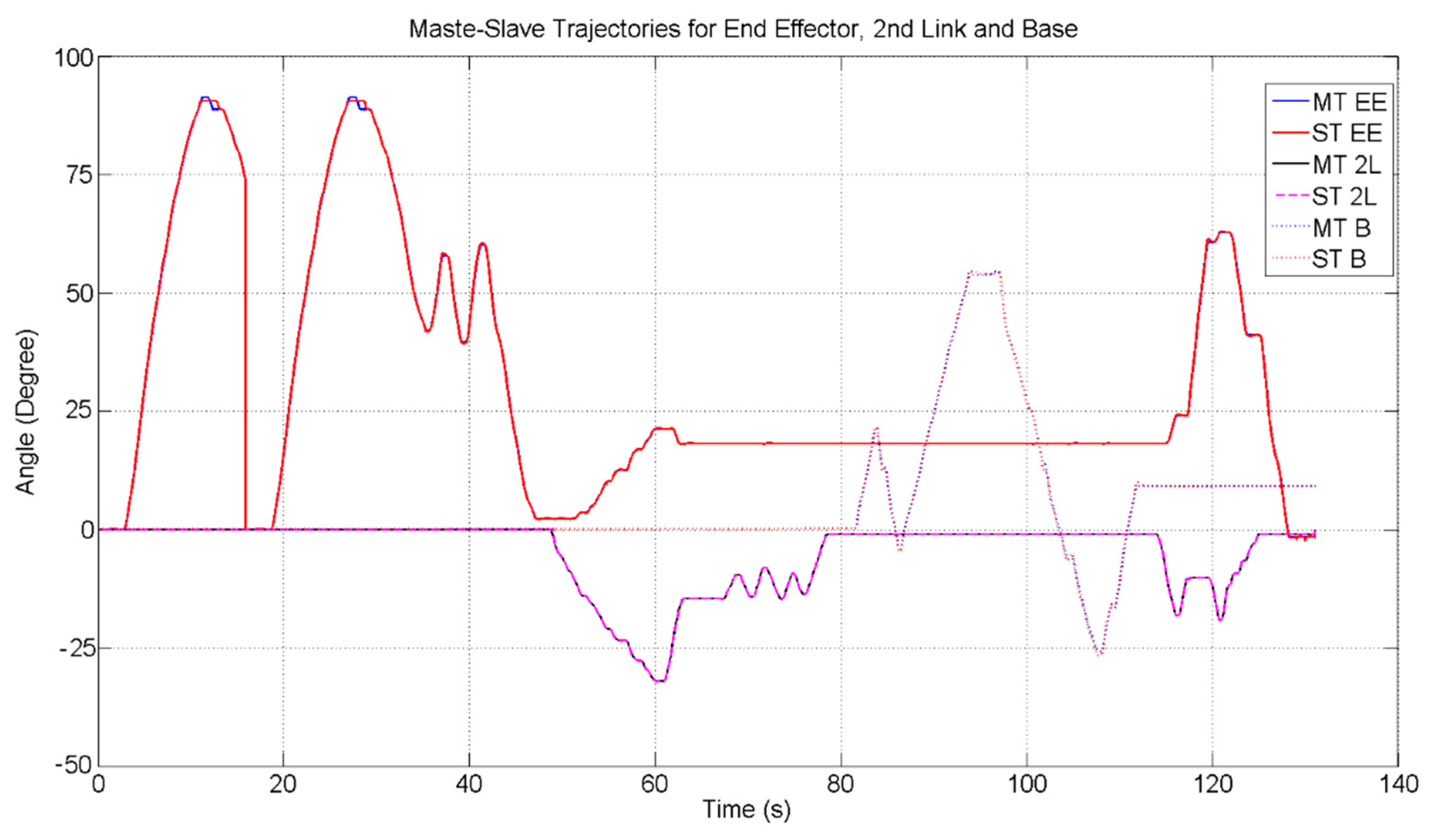
6. Experimental Results

In our study, our system is non-linear, and therefore, a robust control scheme (i.e., SMCSPO) was pursued. Since PID/PD controllers are not robust, comparatively to SMCSPO, to nonlinearities. Therefore, their performance is not as good as that of the proposed SMCSPO. Figure 10 shows the comparison between PID and SMCSPO.

Table 3. Design parameters.

S. No	Parameters	Values
1	k · (End Effector)	25
2	k · (2nd Link)	250
3	k · (Base)	8
4	k1	39
5	k2	507
6	${\epsilon }_0$	1
7	$c$	13
8	$e$	1
9	${\alpha }_3$ (End Effector)	4.08
10	${\alpha }_3$ (2nd Link)	10
11	${\alpha }_3$ (Base)	2.58

shows the values of the parameters used in the experiment by using SMCSPO. The parameters used in the experiment are determined by using the Equations (32) and (33). Extensive simulations were performed to find the best value of boundary layer width (${\epsilon }_o$) resulting in convergence of the sliding surface to zero.

Six different experiments are done by using SMCSPO: (i) Bilateral (Master–Slave manipulation) control of the end effector (ii), estimated perturbation measured at the end effector of master and slave (iii), bilateral (Master–Slave manipulation) control of the 2nd link (iv), estimated perturbation measured at the 2nd link of master and slave (v), bilateral (Master–Slave manipulation) control of the base (vi), and bilateral (Master–Slave manipulation) control of the end effector, 2nd link and base at the same time.

The scenario of the experiment is set up such that the operator (human) moves the master device and the slave device follows the trajectory of the master device using SMCSPO. Figure 11 shows the experimental result of the master–slave trajectories for the end effector. The blue line shows the experimental result of the master device whereas, the red line shows the experimental result of the slave device by using SMCSPO. It can be observed that the slave device can follow the master device. The maximum value of the trajectory is 81 degree at 14 s. The end effector of the slave device can move between 0 and 90 degrees.

The error between the master–slave trajectories for the end effector is shown in Figure 12. The maximum error between the master and slave trajectories is 0.62 degrees at 15.5 s. It can be seen that the errors between the master and slave trajectories are very small.

Figure 13 and Figure 14 show the estimated perturbation of master and slave for the end effector. The maximum estimated perturbation of the master is 67.56162 N*m at 14 s. While the maximum estimated perturbation of the slave is 1516.7 N*m at 14 s.

The value of the estimated perturbation for the slave is very high as compared to the master. This is because of the hydraulic system for the slave. The dynamic value of the slave (i.e., 303.26) is much bigger than the master (i.e., 1.35135). The pattern of the estimated perturbation of master and slave is the same but in an opposite direction. To compare these two results, we normalized the estimated perturbation of master and slave. The normalized estimated perturbation of master is between 0 and 1 while the slave is between −1 and 0 using Equations (49) and (50).

$$P_{norm}(Master)=\frac{a_i-\min (a)}{\max (a)-\min (a)}, i= 1 \dots N$$

(49)

$$P_{norm}(Slave)=\frac{a_i-\max (a)}{\max (a)-\min (a)}, i= 1 \dots N$$

(50)

In the above equations, $a_i$ is the current value. Figure 15 shows the normalized estimated perturbation for the master and slave of the end effector. The red line shows the normalized estimated perturbation of the master device, whereas the blue line shows the normalized estimated perturbation of the slave device.

Figure 16 shows the experimental result of the master–slave trajectories for the 2nd link. The blue line shows the experimental result of the master device, whereas the red line shows the experimental result of the slave device by using SMCSPO. The slave device can also follow the master device. The maximum value of the trajectory is 60 degrees at 13.5 s. The 2nd link of the slave device can move between 0 and 90 degrees.

The error between master–slave trajectories for the 2nd Link is shown in Figure 17. The maximum error between master and slave trajectories are 0.41 degree at 49 s.

Figure 18 and Figure 19 show the estimated perturbation of master and slave for the 2nd link. The maximum estimated perturbation of the master is 326.6367 N*m at 38.5 s. While the maximum estimated perturbation of the slave is 1296.9 N*m at 38.5 s. The pattern of master and slave estimated perturbation is the same but in opposite direction.

Figure 20 shows the normalized estimated perturbation for master and slave of the 2nd link. The red line shows the normalized estimated perturbation of the master device, whereas the blue line shows the normalized estimated perturbation of the slave device.

Figure 21 shows the experimental result of master–slave trajectories for the base axis. The blue line shows the experimental result of the master device whereas, the red line shows the experimental result of the slave device by using SMCSPO. It can be seen that the slave device can follow the master device. The maximum value of the trajectory is 100 degrees at 13 s. The base of the slave device can move between 0 and 360 degrees.

The error between master–slave trajectories for the base is shown in Figure 22. The maximum error between master and slave trajectories is 1.3 degrees at 26.5 s.

Figure 23 shows the experimental result of the master–slave trajectories for the end effector, 2nd link and base by using SMCSPO. The blue line shows the experimental result of the master device whereas the red line shows the experimental result of the slave device of the end effector. The grey line shows the experimental result of the master device whereas the pink dotted line indicates the experimental result of the slave device of the 2nd link. The blue-dotted line shows the experimental result of the master device whereas the red dotted line shows the experimental result of the slave device of the base. At the beginning only, the end effector can move until 49 s. Then, the end effector and 2nd link moved simultaneously by 12 s (i.e., from 50 to 62 s). After that, the 2nd link moved separately by 18 s (i.e., from 62 to 80 s). Then, the base can move by 32 s (i.e., from 81 to 113 s). In the end, the end effector and 2nd link moved again simultaneously by 16 s (i.e., from 115 to 131 s). The slave device followed the trajectory of the master device accurately. The maximum trajectories of the end effector, 2nd link and base are 88, 27 and 52 degrees, respectively.

7. Conclusions

In this paper, we have estimated the reaction force of the end effector and 2nd link for a three-degree of freedom hydraulic servo system with master–slave manipulators using SMCSPO without using any sensors. By using an SMC-based bilateral control strategy and visual feedback, the slave device followed the trajectory of the master device (human operator) with minimum error. Also, bilateral control is used to estimate the reaction force of the master device which is fed back to the operator to handle the master device.

From Figure 11, Figure 16, Figure 21 and Figure 23, it is confirmed that the slave can follow the master trajectories and an operator can easily handle the slave device by feeling the estimated reaction force using the applied SPO when the slave touches an object even if a force sensor is not used.

The maximum error between master and slave for the end effector, 2nd link and base are summarized in

Table 4. Error between master–slave trajectories.

S. No	Links	Maximum Error (Degree)	Maximum Trajectory (Degree)
1	End effector	0.62	81
2	Link 2	0.4	60
3	Base	1.3	100

.

This research is applied for dismantling nuclear power plants, and there are many situations where a human cannot access due to the high degree of radiation and the very long half-lives of the radioactive materials involved. Therefore, the slave device is used for such hazardous locations. It is useful for activities such as transportation of active uranium in nuclear power plants, disposal of an explosive, remote cutting for nuclear power plant dismantling, grinding, etc.

References

1. Fisher, J.J. Applying Robots in Nuclear Applications; Society of Manufacturing Engineers: Dearborn, MI, USA, 1985. [Google Scholar]
2. Clement, G.; Vertut, J.; Cregut, A.; Antione, P.; Guittet, J. Remote handling and transfer techniques in dismantling strategy. In Proceedings of the Seminar on Remote Handling in Nuclear Facilities, Oxford, UK, 2–5 October 1984; pp. 556–569. [Google Scholar]
3. Ma, S.; Hirose, S.; Yoshinada, H. Development of a hyper-redundant multijoint manipulator for maintenance of nuclear reactors. Adv. Robot. 1994, 9, 281–300. [Google Scholar] [CrossRef]
4. Denmeade, T. A pioneer’s journey into the sarcophagus. Nucl. Eng. Int. 1998, 43, 18–20. [Google Scholar]
5. Varley, J. Windscale: Getting down to the core. Nucl. Eng. Int. 1997, 12, 26–28. [Google Scholar]
6. Benest, T. Taking up arms for decommissioning. Nucl. Eng. Int. 2004, 49, 14–16. [Google Scholar]
7. Tachibana, M.; Shimada, T.; Yanagihara, S. Development of remote dismantling systems for decommissioning of nuclear facilities. In Proceedings of the WM’00 Conference, Tucson, AZ, USA, 27 February–3 March 2000. [Google Scholar]
8. Bakari, M.J.; Zied, K.M.; Seward, D.W. Development of a multi-arm mobile robot for nuclear decommissioning tasks. Int. J. Adv. Robot. Syst. 2007, 4, 51. [Google Scholar] [CrossRef]
9. Dubus, G.; David, O.; Measson, Y.; Friconneau, J.-P.; Palmer, J. Making hydraulic manipulators cleaner and safer: From oil to demineralized water hydraulics. In Proceedings of the IROS 2008. IEEE/RSJ International Conference on Intelligent Robots and Systems, Nice, France, 22–26 September 2008; IEEE: Piscataway, NJ, USA, 2008; pp. 430–437. [Google Scholar]
10. Chabal, C.; Proietti, R.; Mante, J.-F.; Idasiak, J.-M. Virtual reality technologies: A way to verify dismantling operations, first application case in a highly radioactive cell. In Proceedings of the ACHI, Digital World, Le Gosier, France, 23–28 February 2011. [Google Scholar]
11. Raju, G.J.; Verghese, G.C.; Sheridan, T.B. Design issues in 2-port network models of bilateral remote manipulation. In Proceedings of the 1989 IEEE International Conference on Robotics and Automation, Scottsdale, AZ, USA, 14–19 May 1989; IEEE: Piscataway, NJ, USA, 1989; pp. 1316–1321. [Google Scholar]
12. Hashtrudi-Zaad, K.; Salcudean, S.E. Transparency in time-delayed systems and the effect of local force feedback for transparent teleoperation. IEEE Trans. Robot. Autom. 2002, 18, 108–114. [Google Scholar] [CrossRef]
13. Lawrence, D.A. Stability and transparency in bilateral teleoperation. IEEE Trans. Robot. Autom. 1993, 9, 624–637. [Google Scholar] [CrossRef]
14. Yokokohji, Y.; Yoshikawa, T. Bilateral control of master-slave manipulators for ideal kinesthetic coupling-formulation and experiment. IEEE Trans. Robot. Autom. 1994, 10, 605–620. [Google Scholar] [CrossRef]
15. Hannaford, B. A design framework for teleoperators with kinesthetic feedback. IEEE Trans. Robot. Autom. 1989, 5, 426–434. [Google Scholar] [CrossRef]
16. Adams, R.J.; Hannaford, B. Stable haptic interaction with virtual environments. IEEE Trans. Robot. Autom. 1999, 15, 465–474. [Google Scholar] [CrossRef] [Green Version]
17. Yang, Y.; Hua, C.; Li, J.; Guan, X. Finite-time output-feedback synchronization control for bilateral teleoperation system via neural networks. Inf. Sci. 2017, 406, 216–233. [Google Scholar] [CrossRef]
18. Truong, D.Q.; Truong, B.N.M.; Trung, N.T.; Nahian, S.A.; Ahn, K.K. Force reflecting joystick control for applications to bilateral teleoperation in construction machinery. Int. J. Precis. Eng. Manuf. 2017, 18, 301–315. [Google Scholar] [CrossRef] [Green Version]
19. Peñaloza-Mejía, O.; Márquez-Martínez, L.A.; Alvarez-Gallegos, J.; Alvarez, J. Master-slave teleoperation of underactuated mechanical systems with communication delays. Int. J. Control Autom. Syst. 2017, 15, 827–836. [Google Scholar] [CrossRef]
20. Mellah, R.; Guermah, S.; Toumi, R. Adaptive control of bilateral teleoperation system with compensatory neural-fuzzy controllers. Int. J. Control Autom. Syst. 2017, 15, 1949–1959. [Google Scholar] [CrossRef]
21. Farooq, U.; Gu, J.; El-Hawary, M.; Asad, M.U.; Abbas, G. Fuzzy model based bilateral control design of nonlinear tele-operation system using method of state convergence. IEEE Access 2016, 4, 4119–4135. [Google Scholar] [CrossRef]
22. Liu, Y.-C.; Khong, M.-H.; Ou, T.-W. Nonlinear bilateral teleoperators with non-collocated remote controller over delayed network. Mechatronics 2017, 45, 25–36. [Google Scholar] [CrossRef]
23. Su, X. Master–slave control for active suspension systems with hydraulic actuator dynamics. IEEE Access 2017, 5, 3612–3621. [Google Scholar] [CrossRef]
24. Kallu, K.D.; Jie, W.; Lee, M.C. Sensorless reaction force estimation of the end effector of a dual-arm robot manipulator using sliding mode control with a sliding perturbation observer. Int. J. Control Autom. Syst. 2018, 16, 1367–1378. [Google Scholar] [CrossRef]
25. Abut, T.; Soyguder, S. Real-time control of bilateral teleoperation system with adaptive computed torque method. Ind. Robot Int. J. 2017, 44, 299–311. [Google Scholar] [CrossRef]
26. Islam, S. State and impedance reflection based control interface for bilateral telerobotic system with asymmetric delay. J. Intell. Robot. Syst. 2017, 87, 425–438. [Google Scholar] [CrossRef]
27. Le, M.-Q. Development of Bilateral Control for Pneumatic Actuated Teleoperation System; INSA: Lyon, France, 2011. [Google Scholar]
28. Patil, M.D.; Abukhalil, T. Design and implementation of heterogeneous robot swarm. In Proceedings of the ASEE 2014 Zone I Conference, Bridgpeort, CT, USA, 3–5 April 2014; pp. 3–5. [Google Scholar]
29. Xu, X.; Cizmeci, B.; Schuwerk, C.; Steinbach, E. Model-mediated teleoperation: Toward stable and transparent teleoperation systems. IEEE Access 2016, 4, 425–449. [Google Scholar] [CrossRef]
30. Sun, D.; Naghdy, F.; Du, H. Time domain passivity control of time-delayed bilateral telerobotics with prescribed performance. Nonlinear Dyn. 2017, 87, 1253–1270. [Google Scholar] [CrossRef]
31. Azimifar, F.; Abrishamkar, M.; Farzaneh, B.; Sarhan, A.A.D.; Amini, H. Improving teleoperation system performance in the presence of estimated external force. Robot. Comput.-Integr. Manuf. 2017, 46, 86–93. [Google Scholar] [CrossRef]
32. Sakaino, S.; Furuya, T.; Tsuji, T. Bilateral control between electric and hydraulic actuators using linearization of hydraulic actuators. IEEE Trans. Ind. Electron. 2017, 64, 4631–4641. [Google Scholar] [CrossRef]
33. Soltani, M.K.; Khanmohammadi, S.; Ghalichi, F.; Janabi-Sharifi, F. A soft robotics nonlinear hybrid position/force control for tendon driven catheters. Int. J. Control Autom. Syst. 2017, 15, 54–63. [Google Scholar] [CrossRef]
34. Wang, Y.; Jiang, S.; Chen, B.; Wu, H. Trajectory tracking control of underwater vehicle-manipulator system using discrete time delay estimation. IEEE Access 2017, 5, 7435–7443. [Google Scholar] [CrossRef]
35. Liu, X.; Jiang, W.; Dong, X.-C. Nonlinear adaptive control for dynamic and dead-zone uncertainties in robotic systems. Int. J. Control Autom. Syst. 2017, 15, 875–882. [Google Scholar] [CrossRef]
36. Li, Y.F.; Chen, X.B. On the dynamic behavior of a force/torque sensor for robots. IEEE Trans. Instrum. Measur. 1998, 47, 304–308. [Google Scholar] [CrossRef]
37. Katsura, S.; Matsumoto, Y.; Ohnishi, K. Analysis and experimental validation of force bandwidth for force control. IEEE Trans. Ind. Electron. 2006, 53, 922–928. [Google Scholar] [CrossRef]
38. Wang, J.; Dad, K.; Lee, M.C. Bilateral control of hydraulic servo system based on smcspo for 1dof master slave manipulator. In Proceedings of the 2017 International Conference on Artificial Lifeand Robotics (ICAROB2017), Miyazaki, Japan, 19–22 January 2017. [Google Scholar]
39. Moura, J.T.; Elmali, H.; Olgac, N. Sliding mode control with sliding perturbation observer. J. Dyn. Syst. Measur. Control 1997, 119, 657–665. [Google Scholar] [CrossRef]
40. Slotine, J.J.; Sastry, S.S. Tracking control of non-linear systems using sliding surfaces with application to robot manipulators. In Proceedings of the 1983 American Control Conference, San Francisco, CA, USA, 22–24 June 1983; pp. 132–135. [Google Scholar]
41. Moura, J.T.; Ghosh Roy, R.; Olgac, N. Sliding mode control with perturbation estimation (smcpe) and frequency shaped sliding surfaces. J. Dyn. Syst. Measur. Control 1997, 119, 584–588. [Google Scholar] [CrossRef]
42. Slotine, J.-J.E.; Li, W. Applied Nonlinear Control; Prentice Hall: Englewood Cliffs, NJ, USA, 1991; Volume 199. [Google Scholar]
43. Cho, T.-D.; Seo, S.-H.; Yang, S.-M. A study on the robust position control of single-rod hydraulic system. J. Korean Soc. Precis. Eng. 1999, 16, 128–135. [Google Scholar]
44. Jelali, M.; Kroll, A. Hydraulic Servo-Systems: Modelling, Identification and Control; Springer Science & Business Media: Berlin, Germany, 2012. [Google Scholar]
45. Lee, M.C.; Aoshima, N. Identification and its evaluation of the system with a nonlinear element by signal compression method. Trans. Soc. Instrum. Control Eng. 1989, 25, 729–736. [Google Scholar] [CrossRef]
Figure 1. Structure of the 3DOF hydraulic servo system.
Electronics 07 00256 g001
Figure 2. The 3DOF hydraulic servo system.
Electronics 07 00256 g002
Figure 3. Schematic diagram of end effector.
Electronics 07 00256 g003
Figure 4. Schematic diagram of base and second link.
Electronics 07 00256 g004
Figure 5. The work flow of control algorithm.
Electronics 07 00256 g005
Figure 6. Master device.
Electronics 07 00256 g006
Figure 7. Slave device.
Electronics 07 00256 g007
Figure 8. Experimental setup.
Electronics 07 00256 g008
Figure 9. Pictorial view of visual feedback.
Electronics 07 00256 g009
Figure 10. Comparison between PID and SMCSPO.
Electronics 07 00256 g010
Figure 11. Master–slave trajectories for end effector.
Electronics 07 00256 g011
Figure 12. Error between master–slave trajectories for end effector.
Electronics 07 00256 g012
Figure 13. Estimated perturbation of master for end effector.
Electronics 07 00256 g013
Figure 14. Estimated perturbation of slave for end effector.
Electronics 07 00256 g014
Figure 15. Normalized estimated perturbation of master and slave for end effector.
Electronics 07 00256 g015
Figure 16. Master–slave trajectories for 2nd link.
Electronics 07 00256 g016
Figure 17. Error between master–slave trajectories for 2nd link.
Electronics 07 00256 g017
Figure 18. Estimated perturbation of master for 2nd link.
Electronics 07 00256 g018
Figure 19. Estimated perturbation of slave for 2nd link.
Electronics 07 00256 g019
Figure 20. Normalized estimated perturbation of master and slave for 2nd link.
Electronics 07 00256 g020
Figure 21. Master–slave trajectories for base.
Electronics 07 00256 g021
Figure 22. Error between master–slave trajectories for base.
Electronics 07 00256 g022
Figure 23. Master–slave trajectories for end effector, 2nd link and base.
Electronics 07 00256 g023