1. Introduction
Wireless Sensors Networks consist of small, independent, and low-cost devices. They are limited in resources such as CPU, memory, bandwidth, transmission range, and power [
1,
2,
3]. The sensor node consists of four components: sensing unit, processing unit, transceiver unit, and power unit [
4]. Sensor nodes sense mostly phenomena such as temperature and humidity [
5] and, in several situations, they are used for tracking and monitoring assets [
6,
7,
8,
9]. Further, sensors in WSNs convert analog signals into digital signals using Analog-Digital-Converter (ADC). Then, the signals are transmitted to the sink node that has no memory or power issue compared to ordinary sensor nodes. The transmission is made through intermediate sensor nodes, which act as forwarders. Security in WSNs is challenging since the network can be utilized in battlefields, border surveillance, building monitoring, hospitals, airports, etc. The information exchange between two sensor nodes or between a sensor node and the sink needs to be secure and confidential. Moreover, the communications between nodes are vulnerable to adversaries who can overhear and analyze the traffic [
10]. Therefore, each sensor node should have the ability to confirm that the message is received from a legitimate node which, is known as integrity. WSNs should be able to avoid spoofing and altering the transmitted packets. Energy is another challenge due to the limitations of the WSNs. They run on batteries and, in many cases, are out of reach [
11]. Accordingly, the security algorithms must be designed in a way to minimize the power consumption while achieving the maximum possible anonymity. Therefore, algorithms should perform reasonable processing and operations not to drain the battery of the sensor node. Since the communications among sensor nodes consume the majority of the power compared to the other sensor components, the overhead should be reduced to minimal. A WSN needs to operate itself after deployment and handle a variety of operations such as the self-network configuration and connectivity maintenance [
12].
Security of WSNs is categorized into content [
13,
14] and context attacks [
15,
16,
17]. Content attacks can be countered by using the confidentiality and integrity in the existing routing protocols [
18,
19,
20] since the adversary focuses only on disclosing the content of packets. Context attacks such as
SLP cannot be protected only by confidentiality and integrity. It requires more convoluted techniques to secure the location of the source as the adversary attempts to locate the source by eavesdropping on the network traffic.
SLP keeps the originator sensor node untraceable and unlinkable. Untraceability means that the adversary is unable to trace back the origin node, whereas unlinkability means that the adversary cannot gain the identity of the source [
21]. In
SLP, the real event (of an asset) mostly has three parameters: event type, event time and, event location [
22]. These parameters are continually targeted by the adversary to gain information about them (
Figure 1).
There are various schemes to overcome context threats from the global adversary model [
1]. For instance, separate path routing allows each packet to travel towards the sink using a different route [
23]; network location anonymization uses a fake identity for the source [
24,
25]; network coding breaks down each packet into smaller pieces that follow different routes to the sink [
26,
27]; and dummy data sources create dummy sources that generate fake traffic, which confuses the adversary about the identity and location of the source [
28,
29]. Using fake traffic is by far the most effective method against global adversaries because it uses different types of packets that appear similar from the outside. In this paper, dummy and fake are used interchangeably. Real packets carry information related to the real event such as its location. Dummy packets do not carry any information about the real event. They are often utilized to mislead the adversary [
1]. In some cases, corrupted packets are injected into the network by an adversary (Injected) or by modifying the existing real or fake packets (Modified) [
30].
Figure 2 shows the different types of packets.
Adversary capabilities are very critical and essential. Encountering a local adversary that has limited resources and a partial view of the network is completely different from a global adversary that has sophisticated resources and full view of the network. In a local adversary model, source anonymity is calculated by the safety period [
31], which means how long the adversary takes to expose a source node; longer time indicates more privacy. The safety period measurement is fine if the adversary is local. However, it is not valid when the adversary is global as the adversary has the ability to perform complex techniques such as rate monitoring and time correlation attacks [
28,
32,
33,
34,
35].
Adversaries can employ two types of attacks: active and passive [
27,
36]. An active attack occurs when the adversary attempts to alter the network traffic by modifying the packets’ header, the packets’ content, or even by injecting new packets into the network to apply some attacks such as Denial-of-Service (
DoS). In contrast, a passive attack occurs when an adversary analyzes the network traffic without alteration by observing which sensor nodes are transmitting and which sensor nodes are not. A passive attack is more difficult to detect than an active attack because no modifications are noticed by the system. This work attempts to defend against passive attacks.
The rest of the paper is organized as follows.
Section 2 discusses the background.
Section 3 describes the existing dummy packet techniques.
Section 4 provides a classification for privacy techniques using dummy packets injection.
Section 5 discusses the global adversary models.
Section 6 provides a classification of the global adversary models.
Section 7 presents the conclusion.
2. Background
Security in WSNs has been a challenge because of the unique aspects they have. It is unsatisfactory to use the ordinary security mechanisms in WSNs due to the limitation of resources such as processing power and battery life. Sensors are independent and do not normally follow a central control entity because of their large scale and frequent topology changes. Therefore, traditional security solutions are inapplicable since they require significant overhead and sufficient memory. One of the basic defenses against security attacks is to prevent the access to network nodes physically. This is impractical in WSNs as many applications require sensor nodes to be deployed in remote and open locations that are difficult to reach, control, manage and protect from unauthorized physical accesses. Packets in WSNs are vulnerable. They can be lost or corrupted because of routing failures or collisions. Such challenges must be taken into consideration when developing security protocols for WSNs [
37].
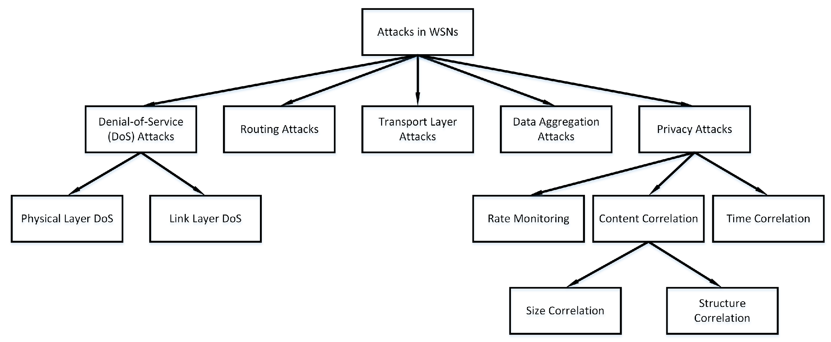
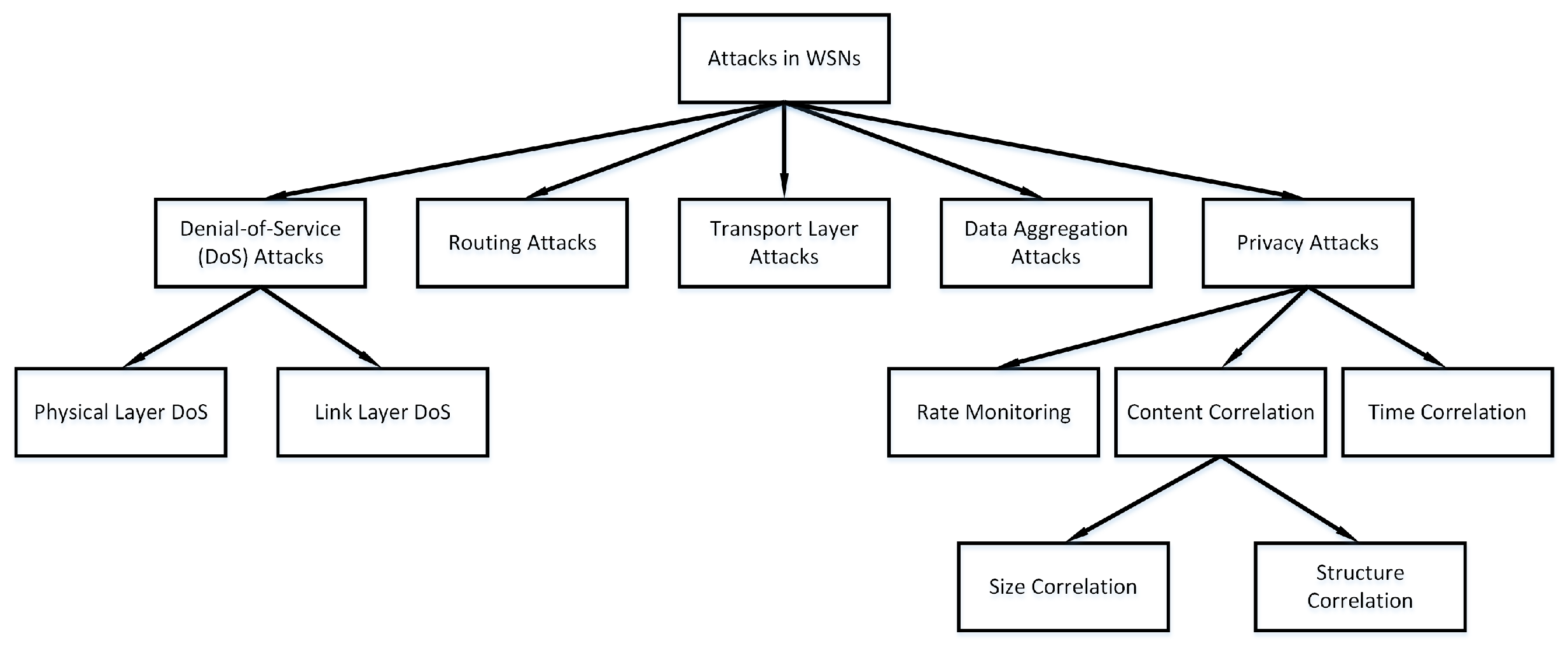
There are several kinds of security attacks against WSNs such as
DoS, routing attacks, transport layer attacks, data aggregation attacks, and privacy attacks, as depicted in
Figure 3.
DoS occurs when an adversary prevents the network from functioning or providing the expected services to applications.
DoS could attack the physical layer and link layer. One of the attacks on the physical layer is the
Jamming attack where an attacker interferes with radio frequencies of the sensor nodes to prevent them from transmitting and receiving meaningful data.
Tampering attack is also a physical layer attack that attempts to destroy or modify the sensor node physically. This attack might lead the adversary to obtain sensitive information which could compromise the entire network. A
Collision attack is a link layer attack that interferes with packet transmissions to make the network re-transmit the same packets repeatedly, which increases the overhead and power consumption [
37].
A variety of routing attacks can be performed by an adversary. For example, a malicious node in the
Blackhole attack and
Sinkhole attack tries to convince the sensor nodes that it is a legitimate data forwarder in the network. Once the malicious node receives the packets, this node drops them right away. Another attack is the
Selective Forwarding attack, which is very similar to the
Blackhole attack and
Sinkhole attack. The only difference is that
Selective Forwarding attack discards a certain number of packets based on specific criteria rather than dropping all incoming packets. Some other attacks target the on-demand routing protocols such as the
Rushing attack. In this attack, the malicious node forwards all incoming route requests to nearby nodes without using the actual routing protocol policies, which involves more nodes in the route. Location-based routing protocols are weak against the
Sybil attack that provides the adversary with multiple identities at different locations in the network. Legitimate nodes will think that the malicious node is one of its trusted neighboring nodes and start forwarding packets to the malicious node.
Wormhole is another attack on routing. The
Wormhole attack occurs when the malicious node has more capabilities than other nodes in the network, such as bandwidth. This increase in capabilities might attract authorized nodes to forward their data to the unauthorized node since it has a high-speed connection. The
Wormhole attack could help other attacks such as
Blackhole to take place [
37].
Transport layer protocols such as Transmission Control Protocol (
TCP) and User Datagram Protocol (
UDP) are vulnerable to the
Flooding attack. A protocol such as
TCP keeps state information allowing the adversary to send multiple connection requests that waste memory and reject any future connection requests even from authorized nodes. The
Desynchronization attack attempts to block the transmission between two nodes by sending fake messages using a modified sequence number to both parties making each node believe that its packet has not been delivered. Therefore, a re-transmission is needed causing unnecessary overhead [
37].
Data aggregation works by combining duplicated data from multiple sensor nodes to reduce the overhead and redundant information. There are many aggregation functions such as
Sum,
Average,
Count,
Max, and
Min that can be easily modified by the adversary to make the network act differently [
37].
Privacy attacks focus on analyzing the traffic of the network [
15,
16,
17,
38]. An adversary can obtain critical information by snooping on the network. The nature of WSNs facilitates attackers to monitor and capture the traffic between sensor nodes. Traffic analysis allows the adversary to identify the most important nodes in the network such as source and sink nodes or gain information about the hot-spot and high traffic regions in the network, known as the
Rate Monitoring attack.
Time Correlation is another privacy attack that monitors the difference between transmitting times of packets and if the network packets follow a specific distribution type in trying to find the relationship, e.g., transmitting times between real and fake packets. This could lead to exposing the location of the source node. Another attack is the
Size/Structure Correlation, which focuses on the size and payload structure of packets to observe any differences. This work focuses on providing techniques that prevent privacy attacks against source nodes.
There are many protocols in the literature that counter global adversary models. Dummy packet injections is one of the most effective methods against the global adversary model. The global adversary has unlimited power, sufficient resources, and the ability to analyze the entire network, which makes the adversary difficult to be defeated. Other techniques such as Separate Path Routing (
SPR), Network Location Anonymization, and Network Coding try to modifying the routing protocol, transmitting the packets using different paths, or use pseudonyms to hide the identity of the source node. These techniques would work defending against local adversaries who have a partial view of the network, limited power, and resources. Nevertheless, they are not effective against the global adversaries [
1]. Global adversaries need more sophisticated schemes to be encountered. Letting some nodes transmit fake packets along with real one could create a confusion from the global adversary perspective. Even if the global adversary has a full view of the network, it is not straightforward to trace back the origin and detect the real event because they have multiple paths and combinations to calculate. They need to apply complex rate monitoring and time correlation attacks to get near the source node.
Dummy packet injection techniques have a massive impact on defending against global adversary models. They might be the most effective solution to counter a well-equipped attacker. Dummy packet injection techniques use a mix of real and fake packets to mislead the adversary away from the source node, unlike other methods that use only real packets. Dealing only with the packets of the real event can limit the countering options since the adversary knows the occurrence of the real event in advance. The general notion behind such techniques is to inject the network with fake packets. Fake packets are identical to the real ones regarding the size and structure to avoid any size/structure correlation attacks. Usually, fake packets are transmitted from several sensor nodes in different places within the network whenever a real event is detected. In some techniques, they generate and transmit fake packets even if there are no real events to add more uncertainty from the attacker perspective. The injection of dummy traffic is according to a specific set of rules. Some techniques simulate the movement of an asset in a different location in the network, which confuses the adversary about the actual location of the real event, whereas other techniques transmit fake packets periodically to confuse the adversary about the existence of the real event. Moreover, several techniques use fake clustering to create different hot spots during the real event transmission. Nevertheless, the main disadvantage of the dummy traffic techniques is the overhead caused by the dummy traffic. The higher is the dummy traffic, the greater is the protection of the source node. Otherwise, the real event can be easily detected by an adversary. One more obvious disadvantage is the incurred processing time due to the fact that the sensor nodes must manage the flows of real and fake packets. In addition, power consumption can be another drawback because of the overhead and increased processing time.
3. Dummy Packets Techniques
In this section, we present the existing techniques in the literature, which rely on dummy packets against the global adversary model. All techniques in this survey are utilized in monitoring and tracking applications. For example, tracking endangered species in a national park, a soldier on a battlefield, a patient in a hospital, etc. The location of the asset needs to be securely communicated to the base station, which means it is untraceable under any traffic analysis applied by an attacker. Traffic analysis can be rate monitoring, time correlation attacks, and size/structure correlation attacks.
3.1. Periodic Collection (PeCo)
PeCo [
39] is one of the first techniques that introduced the concept of fake packets against global adversary. This technique works as follows: each node in the network must obtain a shared individual key between itself and its neighboring nodes for encryption purposes. When the sensor node receives a packet, it decrypts and adds the packet to its buffer using the First-In-First-Out (
FIFO) queuing mechanism. Every node has a timer that counts down; once the timer reaches zero, the first real packet in the buffer is encrypted and sent to the destination. However, if there is no real packet, a fake packet is generated and sent instead. On the receiving side, if a node received a fake packet, it discards the packet instantly. The main issue in
PeCo is the buffer size. The network nodes should have a sufficient buffer size to manage all incoming packets. The Overhead of power consumption and latency are considered serious issues in
PeCo because the nodes generate a fake packet whenever there is no real packet to transmit.
3.2. Constant Rate (ConstRate)
The fundamental concept of
ConstRate [
32] is to divide the lifetime of the network into intervals. Packets are only sent or forwarded at these intervals whether they are real or fake to make them indistinguishable. If a node does not have a real packet to transmit during the interval, a fake packet is transmitted instead. However, the use of intervals concept increases the latency. In addition, this technique has a high power consumption due to the number of fake packets created to protect the real traffic.
3.3. Probabilistic Rate (ProbRate)
The difference between
ProbRate [
32] and
ConstRate is that
ProbRate selects the next interval to send or forward packets based on exponential distribution to reduce the delay and number of fake packets. However, if the adversary knows
, which is one over the transmission rate, and it is the only parameter in the exponential distribution, the network might be compromised. Therefore, the random number that is used to generate
needs to be protected and unknown to adversary.
3.4. Fitted Probabilistic Rate (FitProbRate)
FitProbRate [
32] uses the same exponential distribution as
ProbRate to generate dummy traffic. If a node detected a real event, it transmits real packets following the exact exponential distribution of the fake packets. Therefore, the adversary would be unable to distinguish the difference between real and fake packets. To reduce the traffic overhead, the transmission rate should be as low as possible; in return, this small transmission rate increases the delay relatively.
The network nodes generate a random number utilizing a unique seed to predict the following sending time interval. The seed can be known to the adversary, whereas the random number must be hidden. When a real event occurs,
FitProbRate must use the same
of the fake packets exponential distribution to avoid any
Time Correlation attacks by the adversary. Concurrently, packets of the real event should be transmitted as soon as possible. Therefore,
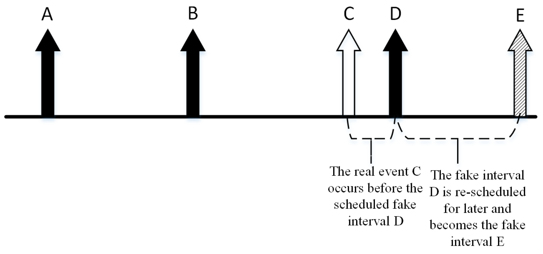
FitProbRate employs the Anderson Darling test (
A-D) to determine whether a series of intervals follow the exponential distribution. This is achieved by searching the first appropriate time interval that satisfies the
A-D test, which at the same time does not break the exponential distribution sequence for the real packets. In case there is a scheduled fake interval, it is replaced by the real one. The fake interval will be rescheduled for later, as shown in
Figure 4. Interval D is the fake one and it will be replaced by interval C, which has the real packet. Then, the fake packet in interval D will be rescheduled for transmission in interval E.
The disadvantages of this technique are as follows: First, it has significant traffic overhead that reduces the lifetime of the network. Second, using the A-D test every time a real event is detected increases power consumption and processing time. Lastly, transmission rate and delay cannot be controlled since FitProbRate does not provide a mechanism to ensure the maximum required delay by intolerant applications.
3.5. Baseline
In the
Baseline [
33] technique, each node in the sensor network transmits real or fake messages pursuing a constant or exponential distribution. When a node detects a real event, it does not transmit the message immediately. Instead, the node waits for a while to ensure that the real packet follows the same distribution as the fake packets. As a result, the adversary cannot recognize the difference between real and fake events. However, this technique is very expensive for the network because it adds a massive amount of traffic overhead and decreases the delivery ratio of real packets since
Baseline uses intervals to deliver the real event.
3.6. Proxy-Based Filtering (PFS)
To overcome the issues of the
Baseline technique such as high overhead and poor delivery ratio,
PFS [
33] was introduced. The primary concept of
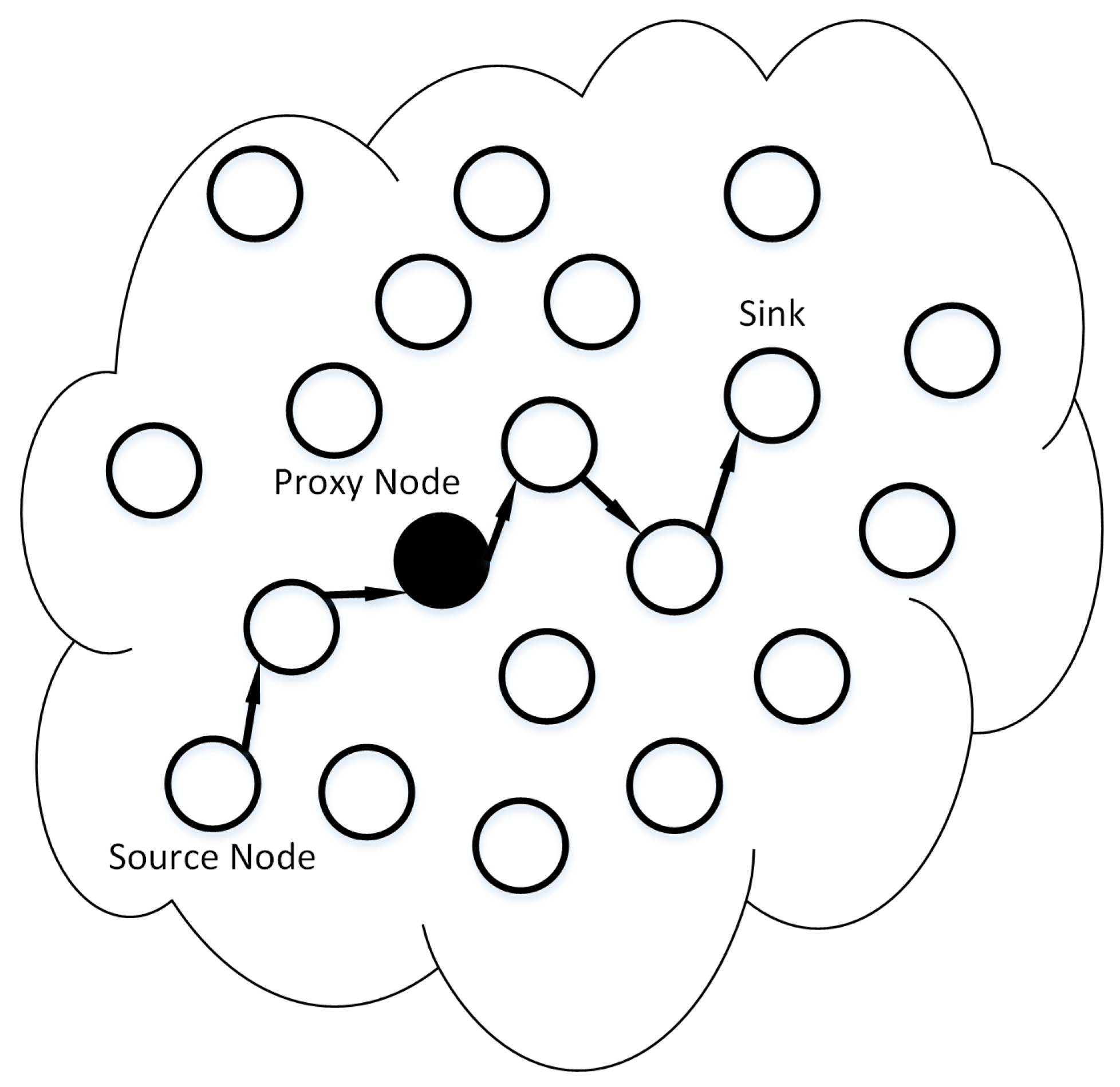
PFS is to hire some of the sensor nodes to act as designated proxies. These proxies filter the fake packets towards the sink, which reduces the overhead traffic while keeping the source anonymity.
In
PFS, some of the sensor nodes are selected to filter the fake packets from neighboring nodes, as shown in
Figure 5, which reduces the overhead as many of the fake packets are dropped before reaching the sink. The proxy node filters the packets to decide which packets will be forwarded and which packets will be dropped.
PFS relies on the location of the proxy nodes; therefore, a proxy placement algorithm is performed to minimize the overhead of the network. Further,
PFS should select the values of the proxy parameters such as the buffer size. This selection is necessary to handle the transmission delay of the real event at the source node. Yang, Y. et al. [
33] claimed that the
PFS technique provides a nearly optimal proxy placement, high delivery ratio, and low bandwidth overhead.
The PFS technique divides the network into cells (groups of nodes) that allow every two nodes in neighboring cells to communicate directly with each other. When an event is detected, it belongs to the cell, not to the node. Each cell has a coordinator node that is responsible for all actions within the cell. A unique ID is assigned to each cell in the network. A node recognizes its cell by using a GPS or an attack-resilient localization scheme. The sink is assumed to be in the center of the network, and each event has a cell ID, event type, and event time.
After proxies have been selected, they broadcast a “hello message” that includes Time-To-Live (TTL) value which has the ability to reach all cells in the network. Next, each cell records the nearest proxy based on the received “hello message” and assigns the selected proxy as the default one for future communications. Then, every cell responds back to the selected proxy to inform the proxy that it is the one selected by the cell. Each cell creates a pairwise key with its proxy using one of the keying schemes. In addition, each proxy has a shared key with the sink. When a cell has a message to transmit, this message is encrypted using the pairwise key and sent after encryption to the proxy using multi-hop routing protocol such as Greedy Perimeter Stateless Routing (GPSR). However, these messages follow the exponential distribution whether they are real or fake to avoid any Time Correlation attacks by an adversary. Therefore, if a cell observed a real event, the real event is delayed until the cell finds the appropriate time interval that does not violate the exponential distribution. When a proxy receives a fake packet, it discards the packet immediately. However, if the received packet is a real packet, the proxy re-encrypts the packet using the key shared between itself and the sink. Then, the proxy forwards the packet after delaying it in its buffer for an appropriate time. In the case the proxy node did not receive a real packet for some time, it transmits a fake packet to the sink instead.
Note that a proxy node is able to recognize the difference between real and fake packets. Moreover, if a proxy receives a packet from another proxy in the network whether the packet is real or fake, the proxy forwards the packet to the next hop without filtration. A message routes through multiple proxies on its way to the sink; however, it is only being filtered in the original proxy. Eventually, optimizing locations of the proxies is essential to avoid undesirable traffic overhead. A disadvantage of this technique is that the sink must be in the center of the network. Another disadvantage is the filtration delay as the packet has to be filtered by a proxy before arriving at the sink.
3.7. Tree-Based Filtering (TFS)
TFS [
33] is an improved version of
PFS. The difference between them is that
TFS has several layers of filtration, and the proxies nearest the sink filter fake packets coming from the proxies that are far from the sink, which leads to less overhead. In
TFS, each proxy has a parent proxy and can have some child proxies using a tree concept to decrease the number of fake messages towards the sink. In contrast, more delay is required because the message is delayed in each and every proxy towards the sink. Therefore, the relationship can be described as a trade-off between overhead and delay while keeping high anonymity. Nevertheless, assuming the sink node is in the center of the network will limit the applications that can implement this technique. Using multiple proxies for filtration might also impact the performance of
TFS.
3.8. Optimal-Cluster-Based Source Anonymity Protocol in Delay-Sensitive Wireless Sensor Networks (OSAP)
Techniques such as ConstRate and FitProbRate provide source anonymity but they are costly since they inject the network with a large number of fake messages. Further, all nodes in the network transmit traffic towards the sink that causes the network to be imbalanced as nodes closer to the sink consume more power than nodes far from the sink, which leads to a shorter lifetime of the network.
To overcome the high overhead in
ConstRate and
FitProbRate, and latency in
PFS and
TFS,
OSAP [
40] was developed.
OSAP is based on
FitProbRate and Niu, X. et al. [
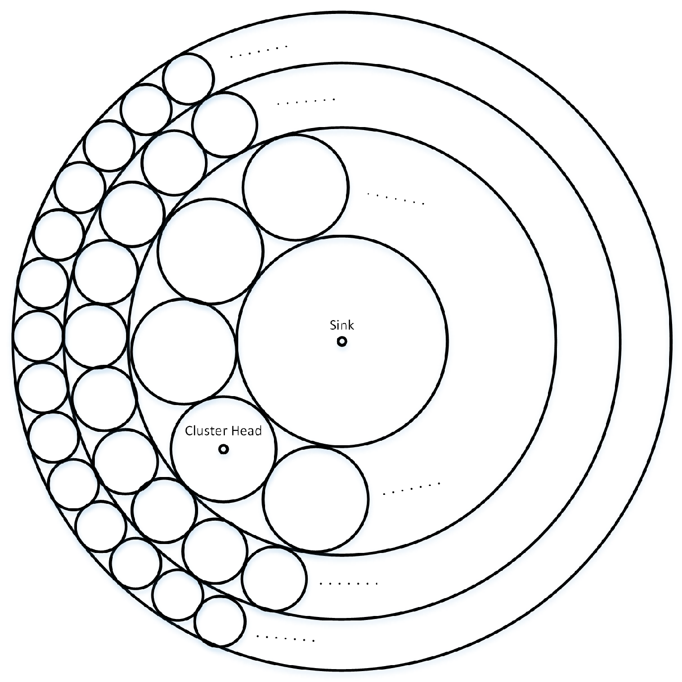
40] argue that the use of unequally clustering mechanism will reduce the traffic overhead, improve the network balance, and decrease the latency of the real event. The unequally clustering mechanism is achieved by adjusting the transmission rate and the radius of unequal clusters. As a result, this mechanism fixes the overhead issue by transforming the issue into a mathematical programming problem that is solved by mathematical methods.
If a node has a real event to report, it becomes a source that generates some real packets, unlike
FitProbRate, which allows all nodes to transmit packets whether they are real or fake. In addition, authors of
OSAP assumed that the sink is placed in the center of the network and works as the data collector for all events. Each packet has a source
ID, event description, event time, and packet type (real or fake). Each node determines the number of hops to the sink by using the following formula:
where
n is the number of hops,
r is the transmission range and
is the network density of nodes distribution. After a node knows its hops count to the sink, the sensor network is divided into uneven clusters. Clusters, which are close to the center of the network are larger than the ones that have a further distance from the center, as shown in
Figure 6. The sink node has the largest cluster and nodes at edges of the network have the smallest clusters. Nodes are categorized into cluster heads and cluster members. The purpose of the cluster head is to filter the incoming fake packets and forward the real packets of the cluster members to the sink. The cluster head of the cluster with radius
is the sink and all nodes within this cluster transmit their packets directly to the sink. All nodes with distance
,
, ...,
are cluster head candidates that have cluster radius of
,
, ...,
, respectively. After cluster head nodes are selected, they broadcast BEACON packets with
TTL, which includes the radius of the clusters they belong to. Member nodes select their cluster head based on the least communication cost, which is decided by the received BEACON packets. Then, each member node notifies its selected cluster head by a BEACON response. Therefore, the network will consist of rings and each ring consists of clusters. The distance between cluster head nodes and the sink is
,
, ...,
.
This technique assumes that each member node shares a pairwise key with its cluster head using a keying scheme. Each cluster head shares a key with its neighboring cluster head nodes. Once the member node detects an event, it sends the event to its cluster head using a multi-hop routing protocol. The member node delays the real packet to the next interval. Therefore, the adversary cannot distinguish the real packets from the fake ones using time analysis. Then, the cluster head decrypts the message and forwards it to the next cluster head encrypted by the shared key between them. To satisfy source anonymity, the transmitting time intervals follow the exponential distribution as exhibited by the FitProbRate technique. When a fake packet is received by the head cluster, it is discarded. In contrast, if the cluster head received a real packet, it re-encrypts and forwards the packet towards the sink after an appropriate time that follows the exponential distribution. However, if there is no real packet, the cluster head sends an encrypted fake packet instead. In case a cluster head received a packet from another cluster head, it forwards the packet after an appropriate time whether it is real or fake without filtration. The total delay of the real event must be less than the maximum required delay by the application. In addition, it is obvious that member nodes at the edge of the network have more cluster heads on the path to the sink, which increases the delay. Therefore, selecting the appropriate for each cluster is mandatory to balance the latency between clusters and to avoid any time analysis attacks from the adversary. Finally, balancing the power consumption between clusters is made by adjusting the radius of the unequal clusters and transmission rate.
OSAP still has some limitations; it assumes that the sink location is in the center of the network. This assumption is impractical for many applications that require the sink to be at different locations in the network. Another limitation is that the communications within the network are based on the same cluster heads that do not change during the lifetime of the network. Using the same cluster heads every time decreases the lifetime of the network because the cluster heads will consume more power than cluster members causing the network to be imbalanced regarding power consumption.
3.9. Recurrent Clustering Mechanism (RCM)
The reason many techniques are not very practical is because the nodes near the sink consume more power than the nodes far from the sink,
RCM [
41] authors argued. To balance the network, a clustering technique was introduced. All nodes use the
FIFO queuing mechanism. Each cluster has a cluster head that coordinates the activities within the cluster. Each node has a timer, once the timer is equal to zero, the sensor node checks if it has a real packet in its buffer to transmit. In the case there is no real packet, a fake packet is sent instead to the sink. The remaining energy of cluster heads is computed every time there is a packet to transmit. The higher cluster head in terms of the remaining energy is selected to forward the packet. In this technique, the sink location is known to the adversary. Since this technique uses clustering and selects the highest cluster node with the remaining energy,
RCM improves the power consumption by half compared to other techniques, George, C.M. et al. [
41] argued. Moreover,
RCM reduces the overhead because of the clustering mechanism. However, George, C.M. et al. [
41] did not mention how they control the delay and delivery ratio. Overhead is still a concern because every time the node does not have a real packet, it generates a fake packet instead, which might lead to traffic overhead.
3.10. General Fake Source (GFS)
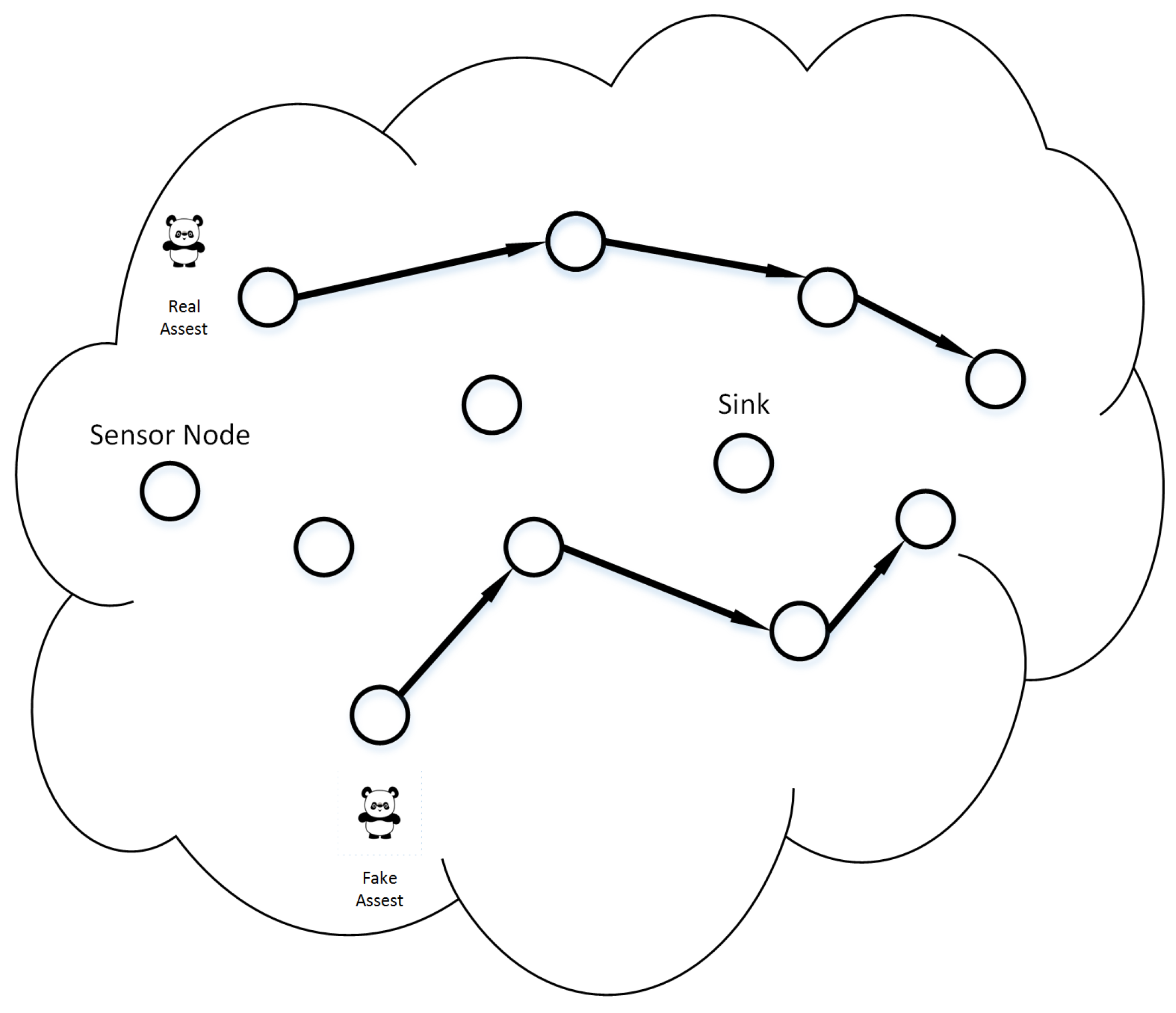
The
GFS [
42] technique attempts to simulate the movement of a real asset at different locations in the network to mislead the adversary about the actual location of the source node, as shown in
Figure 7. This mechanism can be implemented easily if the
RFID type is active. However, the goal of
GFS is to simulate the movement of the asset using a passive
RFID.
GFS generates dummy traffic of a fake source. A shared token is used to determine which node should act as a fake source. Then, the fake source generates a fake event just after detecting the real asset. Next, the token is passed between nodes to simulate the movement of the real asset. To simulate a real asset, the number of intervals, which is represented by
simulateRound, that a fake source will transmit should vary from node to node, to mislead the adversary. Another variable is the
realCount; it is increased by one whenever a node sends a real message. Once a node stops sending real messages, the
realCount is reset to one, and
simulateRound is updated.
The fake source is selected randomly and generates fake messages until simulateRound becomes zero; then, the token is passed. However, to avoid passing the token between only two nodes, the last fake source is recorded in the preNode variable. When the fake source has a real message, the sink should be informed and the token is passed to the next node. Further, if there are real or fake messages without a token, the message can be passed normally to the sink. However, if the fake message has a token, the receiving node will get the preNode and tokenID. Then, the receiving node becomes the new fake source.
Since the token creates extra traffic that might be noticed by the adversary, each fake source needs to send a fake report to make the token message look like an ordinary real report. Eventually, real and fake messages have to be transmitted together in every interval to distract the adversary. However, GFS has some drawbacks: First, it assumes that the sink is placed in the center of the network. Second, if the token is passed among three nodes or more rather than between two nodes, there is no mechanism to handle this kind of situations. Third, GFS could fail to provide anonymity because only fake messages are created when a real event takes place. Therefore, the adversary might detect that a real event is being sent resulting in exposing the location and time of the event in case the adversary has enough capabilities and resources to examine all nodes at once.
3.11. Naive Algorithm (NAA)
Each node in
NAA [
43] broadcasts a fake message periodically. The time duration of these periods should be long enough to avoid draining the battery quickly. If a node has a real message to transmit, it waits until the upcoming fake message is ready. However, instead of transmitting the fake packet, it is replaced by the real message. Once the real message is received by intermediate nodes, the process is repeated until the real message reaches its destination. The adversary cannot distinguish the difference between real and fake messages since they are sent using the same transmission rate. Nevertheless, the delay in this technique is high because it uses fixed long periods to transmit real messages.
3.12. Globally Optimal Algorithm (GOA)
The
GOA [
43] technique is an upgraded version of
NAA. It was developed to decrease the delay of the real event.
GOA provides each node with a timer that is defined by a pseudo-random number generator. This timer is utilized to allow the node to transmit real packets. If the time count reaches zero, and there is no real packet to transmit, a fake packet is transmitted instead. All nodes must use the same pseudo-random number generator to confuse the adversary and obtain the seed used by other nodes. This concept allows
GOA to decide the shortest path to the sink. The
GOA technique improves the throughput and power consumption when compared to
ConstRate. However, the primary issue in
GOA is that it should have a knowledge of the entire topology of the network, which is not required by
ConstRate.
3.13. Heuristic Greedy Algorithm (HGA)
The
HGA [
43] technique is very similar to
GOA, but
HGA only needs to obtain the seed and location of neighboring nodes allowing each node to select the best neighboring node to send or forward the packet.
3.14. Probabilistic Algorithm (PBA)
The
PBA [
43] technique is developed to reduce the overhead of dummy traffic in
GOA and
HGA. It follows the same process as
HGA. However, nodes do not have to transmit a fake packet every time the time count reaches zero in case there is no real packet to transmit.
PBA uses a probability
p to decide whether the node should send a fake packet or not;
p is considered as a threshold and used to a trade-off between anonymity and overhead.
3.15. Distribution Resource Allocation Algorithm (DRAA)
The
DRAA [
44] technique uses the same concept as
ConstRate. Each node in
DRAA measures the best transmission rate for dummy traffic to reduce the overhead of the network. The main purpose of
DRAA is to hide the real traffic with minimal dummy traffic. This mechanism can be achieved without applying the entire process of the original
ConstRate technique. The
DRAA technique provides
SLP with reduced power consumption when compared to
ConstRate according to
DRAA developers.
3.16. Optimal Filtering Scheme (OFS)
The
OFS [
45] technique is based on
TFS and
PFS techniques. Each node in
OFS has the possibility to become a proxy. This method can provide an optimal routing and filtering that eventually leads to optimal lifetime for the network. Once a sensor node is selected to be a proxy, it can use its filtration rules for further optimization to maximize the network lifetime. Moreover, a proxy has the ability to filter packets coming from other proxies, unlike
TFS, where the proxy transmits all incoming packets from other proxies without any filtration. In this protocol, proxies have two options: First, proxies can work individually, which increases the delay and provides a high level of anonymity. Second, they work together to decrease the delay with a low level of anonymity. This technique is considered as a trade-off between delay and anonymity. The challenge in
OFS is to select the best locations for the proxies.
3.17. Aggregation-Based Source Location Protection Scheme (ASLP)
The
ASLP [
46] technique uses similar filtration techniques as
OFS.
ASLP has three phases: fake packets, packet encryption, and data aggregation. In
ASLP, the
WSN is divided into clusters, and each cluster has a cluster head. Cluster heads follow a tree structure scheme to reach the sink. Every cluster member shares a key with its cluster head to encrypt the traffic between them. In addition, nodes communicate with their cluster head using the exponential distribution to reduce the delay and overhead. The exponential distribution is only controlled by one parameter
, which is the transmission rate. Cluster nodes report the event to their cluster head, which also can be the sink node periodically; this period is decided by the value of the period time for reporting the event,
. In the second phase, values of
and
are distributed throughout the network by the sink. In the third phase, the actual data aggregation and reporting take place. A node transmits a real packet whenever it detects a real event to the sink using the exponential distribution. Otherwise, the node transmits a fake packet instead. The cluster heads receive the packet from cluster members and forward it to the sink using an encrypted channel. Values of
and
are utilized in this technique to trade-off between latency and power consumption. This trade-off can be adjusted according to the requirements of the applications.
3.18. Trusted Computing Enabled Heterogeneous (TCH-WSN)
The network in
TCH-WSN [
47] is also divided into clusters. Each cluster contains a high-performance node with two modules: Trusted Platform Module (
TMP) and Mobile Trusted Module (
MTM). These two modules are used to provide data security and integrity. The sink and cluster heads are assumed to have a continuous power supply. The sink communicates with all nodes directly. However, a sensor node communicates with the sink only through its cluster head. The cluster head assigns one of the nodes in its cluster to act as a fake source for a specific duration of time. Then, the fake source transmits dummy traffic to the sink.
3.19. Efficient Privacy Preservation (TESP)
The
TESP [
48] technique uses cluster heads to filter fake packets that are being transmitted to the sink.
TESP consists of three phases: In the first phase, the sink provides public and private keys to each node in the network. The keying mechanism contributed by the sink is based on elliptic curve cryptography, which is preferred over the traditional asymmetric key algorithms. In the second phase, nodes are deployed, organized, and assigned to clusters. All clusters have a cluster head that connects to all other cluster heads as well as to the sink in a tree structure manner. The sink is placed at the root of the tree. Neighboring nodes have a symmetric key between them to communicate securely. In the final phase, each sensor node checks its buffer for real packets. If there is no real packet, the node generates a fake packet encrypted by the public key of the cluster head. However, if the node has a real packet in its buffer, this packet is encrypted by the sink’s public key. When a packet reaches the cluster head, if the cluster head is able to decrypt the packet successfully, that means it is a fake packet. Therefore, the packet is dropped immediately. Each cluster head collects all packets from its cluster members. Then, the cluster head waits for a higher cluster head or the sink to ignite the data collection signal. Once the cluster head receives the signal, it sends the collected data after re-encryption to the higher cluster head or the sink. In the case a higher cluster head received data from a lower cluster head, it adds its collected data to the incoming data. This process is repeated until all collected data reaches the sink.
3.20. Cloud-Based Scheme for Protecting Source-Location Privacy (CSPSLP)
Mahmoud, M.E.A. et al. [
49] in
CSPSLP assumed that multiple sensor nodes detect the asset, and these nodes attempt to inform the sink about the location of the asset simultaneously, which creates a traffic hot-spot. Normally, the adversary seeks hot-spot areas to discover the source node. The main aim of
CSPSLP is to hide the actual source inside a cloud that consists of multiple nodes. Therefore, the real hot-spot is hidden within a larger cloud.
CSPSLP consists of three stages: In the first stage, each node is assigned a unique
ID, a secret pairwise key with its neighboring nodes, and a shared key with the sink. These
ID and keys are used by nodes to build pseudonyms that are very similar to the hidden identities utilized in Anonymous Path Routing
APR.
The second stage is executed at the deployment of the nodes, and it is called the bootstrapping stage. In this stage, each node sends its location to the sink to obtain the shortest path between itself and the sink. The following step is to select some of the nodes randomly that are at most h hops away from the sensor node itself. These selected nodes become fake sources, and they exchange data with each other to create pseudonyms among them. Each node separates its neighboring nodes into different groups. All created groups are placed in opposite directions from each other. Further, every node shares a secret key with each group.
The third stage is the event transmission. When a source detects a real event, it decides which node will act as a fake source. Furthermore, the source node broadcasts the packet to one of its groups that was already created. However, the chosen group must have one member on the path towards the selected fake source. The transmitted message contains the actual event encrypted by the pairwise shared key between the source and the sink. Moreover, the pseudonym is shared among the real and fake sources as well as among intermediate nodes, fake sources, real sources, and fake sinks. An intermediate node adds the packet to its buffer only when its pseudonym is in the packet. Otherwise, the intermediate node generates a fake packet with a TLL counter. This packet is forwarded until the TLL counter reaches zero. When the pseudonym of a node is in the packet, the node moves the pseudonym to the next intermediate node and forwards the packet to the group that the node belongs to. All members of the group receive the packet; if the member’s pseudonym is not in the packet, the member generates a fake packet. Nevertheless, if the packet has the pseudonym of the member, the member node adds the packet to its buffer and repeats the process until the packet reaches the fake source. Once the fake source receives the packet, it forwards the packet to the sink using the same process as APR. However, CSPSLP has only one difference from the original APR: CSPSLP re-encrypts the packet that has the event information between all intermediate nodes using the shared key between itself and the sink. When the sink receives the packet, it searches for the pseudonym of the source and the fake source to select the appropriate key to decrypt the packet. Finally, dummy traffic that belongs to the same cloud is filtered by the intermediate nodes. For example, if one of the intermediate nodes had many fake packets from the same cloud, the intermediate node has the right to use a filtration mechanism. This filtration is utilized to only forward one of the fake packets to reduce overhead.
3.21. Dummy Wake-Up Scheme (DWUS)
The key concept of
DWUS [
50] is to create multiple dummy traffic streams to direct the adversary away from the actual location of the source node. These streams have to be toward the sink.
DWUS coordinates the dummy traffic streams to act similar to real traffic streams. This technique consists of three phases: First, the
WSN is divided into different groups of dummy populations. Each group has a group leader that is changed periodically. This group leader is responsible for selecting the fake sources. The second phase is called the Wake-up, each group leader hires a nearby fake source and sends a wake-up message to the selected fake source. In the third phase, once the fake source receives the wake-up message, it sends a fake message towards the sink using one of the selected intermediate nodes. The second and third phases are repeated using a fixed transmission rate to simulate the existence of the real asset at different locations, which subsequently confuses the adversary about the original location of the real asset.
3.22. The Group Algorithm for Fake-Traffic Generation (GAFG)
The fundamental notion of
GAFG [
51] is very similar to
DWUS. Every node in the network transmits its packets to the sink following a predefined path. Forwarding nodes have a higher transmission rate than source nodes. Once a source detects a real event,
GAFG transmits the event to the sink using the exponential distribution. Then,
GAFG attempts to create fake data reports that have a very close
to the real data report. Moreover, this technique ensures that many nodes in the
WSN will transmit fake data at specific times according to the real event exponential distribution. Nevertheless,
GAFG is vulnerable to
Rate Monitoring attacks since forwarding nodes have higher transmission rates than source nodes.
3.23. Source Simulation (SoSi)
This technique [
52] assumes that the global adversary can only trace the presence of a moving asset. The adversary tracks every trace in the network whether it is real or fake. Moreover, each trace is assumed to be a candidate of a real trace. The main aim is to create several traces to mislead the adversary about the presence of the real event. Additionally,
SoSi has its own definition for privacy. Privacy occurs when the adversary observes a set of transmissions, which indicates that the asset is nearby one of the nodes. Virtual assets are created to copy the behavior of the real asset to confuse the adversary. Another purpose of these virtual assets is to create dummy traces. To implement the virtual assets, some sensor nodes are selected randomly. Each selected node obtains a token in the deployment stage. These nodes are called the token nodes.
SoSi forces the
WSN to function in rounds; each round has a fixed time. In each round, a fake event is transmitted to the sink by the token node through its neighboring nodes, which create a stream of traffic. By the end of each round, the token node selects the next node that will act as a token node. The
SoSi technique does not increase the delay since the dummy streams do not affect the real event. However, the use of dummy streams increases overhead.
3.24. Source and Destination Seclusion Using Clouds (SECLOUD)
The
SECLOUD [
53] technique has three steps: First step, each node transmits a “hello message” to all nodes in the network using flooding routing protocol. The “hello message” includes a
TTL counter in trying to find the nearby nodes within a specific range
h. These nodes create a cloud; if a node of a cloud desires to transmit, it selects some of the cloud members to act as pseudo-sources. The basic idea of pseudo-sources is to generate fake packets using the same transmission rate as the real source. All fake packets will be dropped by the receivers. The sink has its cloud and uses the same procedure of ordinary nodes. In the second step,
SECLOUD provides the source node with multiple options. The first option is to communicate with the sink using a single path routing algorithm. The other option is to use delegate sources and delegate sinks. In the second option, the source node assigns some of its cloud members to be delegate sources, and the sink assigns some of its cloud members to be delegate sinks. Therefore, packets can travel between the source and sink through delegate nodes. In the last step, the fake sources and fake sinks that are created in the first step can be utilized to transmit dummy traffic between them. This step is essential to hide the real traffic, which confuses adversaries about the location of the real event. However, the utilized mechanism to create fake clouds is not explained in details. Moreover, the use of the cloud concept might increase the power consumption and overhead of the system.
3.25. Unobservable Handoff Trajectory (UHT)
The
UHT [
54] technique has a unique assumption about the adversary. This assumption is that the asset can enter and move to a random point within the network. Nodes have information about the Poisson distribution of assets entering the
WSN. The traveled distance by assets is based on the uniform distribution. In addition, all nodes use the same shared key to encrypt and decrypt messages among them. In this solution, the edge nodes are called the perimeter nodes because they are the first nodes to detect the asset in the network. The perimeter nodes transmit fake messages in case there are no real events detected by them. A fake message should have a
length variable that behaves similarly to
TTL. The next step is to
XOR the fake message with the
ID of the next node that will send the fake message. The fake message is routed to the sink through intermediate nodes. All nodes use a broadcast technique to transmit their messages. Once a node receives a message, it attempts to
XOR the message with its
ID to determine whether the node should generate a fake message or not. If a readable message is the output of the
XOR operation, the
length variable is decreased. In case the
length variable is not zero, the node sends a fake message after
XORing it with the next node
ID. In contrast, if the
length variable is zero, the message is
XOR-ed with the current node
ID. Then, the node transmits the fake message to the sink through intermediate nodes. By sending messages from fake events, the adversary becomes completely confused about the candidate event and whether it is real or fake.
3.26. Pollution Avoiding Source Location Privacy (PA-SLP)
In this technique [
30], messages are transmitted in specific time slots to avoid Time Correlation attacks. In addition,
PA-SLP implements random network coding on the transmitted packets to prevent
Size/Structure Correlation attacks. In
PA-SLP, there are three different types of packets: real, fake, and polluted (packets created or modified by an adversary). Therefore, a mechanism called Triple-Type Homomorphic Signature (
TTHS) was developed to filter the unwanted packets such as the fake and polluted ones. Moreover, a signature equation with a secret key is used to determine the type of the forwarded packets without exposing their contents. If the packet type is real, it will be forwarded to the next node towards its destination. However, if the packet is fake, it will be discarded to reduce the overhead of the network. Lastly, in the case the packet is polluted, it will be utilized to improve the Intrusion Detection Systems (
IDS) by locating the captured nodes. The entire process is employed by intermediate nodes to enhance the overall performance of the network.
3.27. Fortified Anonymous Communication Protocol (FACP)
The
FACP [
34] technique uses intervals and variable-size sub-intervals to divide the time of the network. It provides high anonymity as the technique generates dummy packets in sub-intervals as needed to maintain the average number of dummy packets throughout the network, authors of [
34] argued. However, the protocol works in a way that causes a very low and measured overhead and a higher lifetime for the network. Another advantage of this technique is that it can handle the transmission of multiple packets at once through the network efficiently. In addition to anonymity, it also handles routing privacy, timing privacy, and rate privacy. All the packets whether are real or fake are encrypted. It provides a unique methodology for generating new keys for every transmission so there is no one key used more than once. The framework provides data integrity as well as privacy. The unique contribution is addressing the temporal and rate privacy by using fake messages. This is by making sure that every sensor node has similar transmission rate whether it is close to the sink or at the edge. Calculating a key for every transmission will be time and power consuming but it provides high source anonymity.
3.28. Dummy Uniform Distribution (DUD)
DUD [
55,
56] divides the time into intervals that have the exact duration, and it uses the same transmission rate for both real and dummy packets. A random number is thrown between 0 and 1. If the thrown number is smaller than the threshold, which is the predefined transmission rate, the source node will transmit the first real packet in its buffer at the end of the current interval. However, if the node’s buffer does not have a real packet, it generates and transmits a dummy packet instead. In contrast, if the thrown number is larger than the threshold, the node will not transmit any packets even if it has a real packet in its buffer. This mechanism is provided to confuse the adversary about the presence of the real event. Since the transmitting of the real event is based on a probability, the latency of
DUD could be high. It is solved by increasing the transmitting rate, but this causes higher overhead as the network transmits more dummy packets. This relationship is considered as a trade-off between overhead and latency [
55,
56].
3.29. Dummy Adaptive Distribution (DAD)
DAD [
55,
56] technique is based on
DUD. However, it gives the nodes that have real packets an advantage over other nodes in the network by increasing their transmuting rate by a specific value
x. This decreases the latency without increasing the overhead. However, increasing the transmitting rate could lead the adversary to be notified that a real event is being transmitted by implementing a time correlation attack. Therefore, nodes that have real packets need to decrease their original transmitting rate by the same specific value
x after sending all real packets in their buffers to balance the transmitting rate and make its average equal to other nodes [
55,
56].
3.30. Controlled Dummy Adaptive Distribution (CAD)
CAD [
55,
56] is based on
DAD and
DUD. It is developed to guarantee the maximum delay of a real event. It forces a node to transmit its real packet if the node failed to transmit using probability within a predefined consecutive number of intervals. Adjusting this number is critical because, if it is large, this provides higher anonymity, whereas, if it is small, it decreases the delay. The relationship in
CAD is considered as a trade-off between privacy and latency [
55,
56].
3.31. Exponential Dummy Adaptive Distribution (EDAD)
In
EDAD [
57], instead of using a uniform distribution as in
CAD,
DAD, and
CAD techniques, it employs an exponential distribution to reduce the overall overhead of the network. A set of dummy packets is transmitted following the exponential distribution. However, if a real event is detected, the scheduled fake packets will be replaced by the real ones. All nodes in the network use the equation
to predict the next time interval for fake packets. This technique provides a high level of anonymity with reduced overhead. However, it has a higher delay than
CAD since it does not have a mechanism to control the latency of real events.
4. Comparison of Fake Packet Techniques
This section provides a comparison of fake packet techniques regarding the use of:
Intervals,
Timers,
Random Numbers,
Probability,
Clusters,
Proxies,
Constant Distribution,
Exponential Distribution, and
Poisson Distribution. The comparison is presented in
Table 1.
Intervals indicate that the lifetime of the network is divided into time intervals. The duration of the intervals can be equal or unequal based on the implemented distribution.
Timers are utilized as a trigger for a node to transmit either real or fake packets.
Random Numbers decide the probability of a node to transmit a packet.
Probability decides whether a node will transmit a packet.
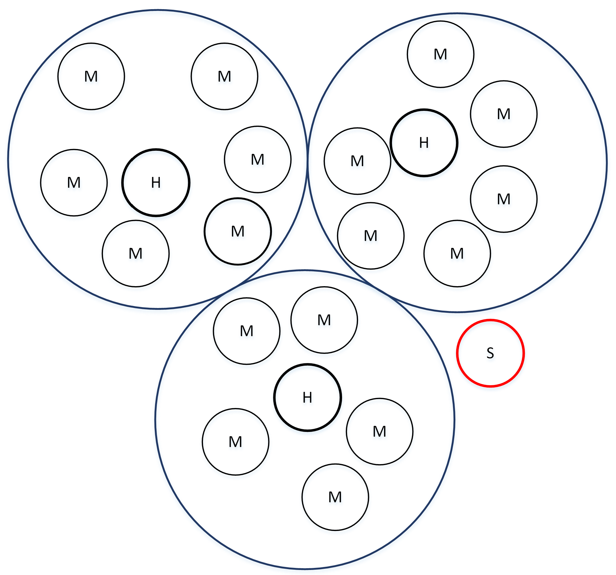
Clusters indicate that the network is divided into groups of nodes (
Figure 8). Each group has multiple member nodes and one head node.
Proxies are commonly used to filter fake packets towards the sink.
Constant Distribution breaks down the time into equal intervals, whereas
Exponential Distribution decides the next interval according to this equation:
, where
X is the next interval,
u is the uniform random number, and
is the transmission rate.
Poisson Distribution calculates its intervals distribution based on the following equation:
, where
is the probability,
x takes a whole number, and
is the average number of events per interval. All techniques are assumed to implement similar structure, format and size for both real and fake packets. Using different size or format for fake packets makes real packets easily detectable if an adversary applies a
Size/Structure Correlation analysis.
5. Global Adversary Models
This section provides a detailed description of the used global adversary models (
Table 2 and
Table 3) in fake packet techniques, and how assumptions are made in each one of them.
The
PeCo technique assumes that the adversary is able to deploy its own sensor network to monitor and analyze a
WSN. Furthermore, the adversary network consists of a smaller number of nodes than the targeted network as the adversary only eavesdrops on the radio signals of legitimate nodes. Additionally, the adversary does not sense the environment, e.g., the authorized nodes. The adversary is also equipped with
GPS to detect the communication locations precisely [
39].
The adversary is considered as
external,
global and
passive in
ConstRat,
ProbRate and
FitProbRate techniques. External means that the adversary cannot control or compromise a sensor node physically. Global means that the adversary has a full view of network communications as well as sufficient resources and unlimited power. Passive has three different aspects: First, an attacker cannot expose the content of a real event message that could lead to the source
ID. Second, in the situation where messages are encrypted the same way during the forwarding process, the attacker has the capability to trace back the origin. Third, the adversary can apply complicated traffic analyses such as
Rate Monitoring and
Time Correlation. In
Rate Monitoring attacks, the adversary focuses on the difference of the transmission rates between nodes, especially those nodes with higher rates. Nevertheless, the
Time Correlation attack works on the diversity of transmission times between transmitting packets. It is also assumed that the adversary has enough resources to apply all of these advanced attacks [
32].
Baseline,
PFS,
TFS and
OSAP techniques have the same assumptions for the adversary, which is
external,
global, and
passive [
33]. However,
OSAP provides more assumptions: First, the adversary knows the location of all nodes in the network. Second, it knows the distribution type of the
WSN. Third, the adversary has the capability to compare its time interval observations with the known distribution type. Additionally, the adversary is assumed to be unable to disclose the content of packets or identify whether the packet type is real or fake [
40].
In
RCM, the adversary cannot decrypt the communications in the network. Therefore, packets appear completely random from the adversary perspective. Moreover, the adversary is aware of the sink location [
41].
The
GFS technique builds its own technique based on the following adversary model assumptions. The adversary deploys its network to overhear the radio transmissions among legitimate nodes. Adversary nodes have unlimited processing power and battery life. The adversary can only eavesdrop on the traffic, but it is unable to alter the traffic or compromise the sensor nodes. Data are encrypted and the adversary cannot gain any meaningful information about the packets’ content. Further, real and fake packets are identical in size and structure making the adversary unable to distinguish the difference between them. Lastly, the adversary has knowledge about the sink location, the network topology, and the implemented routing protocol [
42].
NAA,
GOA,
HGA and
PBA techniques utilize a similar adversary model. This model assumes that the attacker knows the location of all sensor nodes in the targeted network. Moreover, the attacker has the ability to snoop on the traffic of the entire network. The adversary has enough resources to keep all collected data for further offline analyses. However, the attacker is unable to break the encrypted packets or compromise sensor nodes physically [
43].
DRAA,
OFS,
ASLP and
TESP techniques assume the popular
external,
global and
passive adversary model [
44,
45,
46,
48]. However, the adversary in
TCH-WSN can monitor the entire network traffic [
47].
In
SECLOUD, the adversary capabilities are a combination of different adversary models presented in [
39,
58,
59]. In this model, the attacker knows the network topology and retains the measurements of the entire network traffic including
Rate Monitoring and
Time Correlation. In addition, the attacker has the ability to visualize the network traffic and regulate the network links density. However, the adversary is passive and cannot compromise network nodes. The attacker has its own network that consists of several malicious nodes. These nodes collaborate together using a different frequency band to transmit the collected data to a centralized malicious entity [
53].
The
CSPSLP adversary model deploys its monitoring devices in the targeted areas within the network. The adversary collects information from multiple areas, but not from the entire network. These areas are called the observation points, and their location is adjustable to be as close as possible to the real asset. This model has three different characteristics: passive, well-equipped, and informed. Passive means that the adversary does not modify the network transmissions; it only observes transmissions among nodes. Well-equipped means that each attacking device can measure the angle of arrival and strength of the signal to determine the source location. However, the adversary is unable to spot the receiving nodes because all nodes within the range of the transmitting node will receive the signal. Lastly, the adversary is informed; it knows the sink location and is able to monitor the sink node traffic as well [
49].
DWUS assumes that the adversary is passive and has unlimited resources. Further, the adversary can distribute attackers throughout the network to sense all transmitted packets [
50].
In the
GAFG technique, the adversary is aware of the sink location and network topology. The adversary is passive and can detect the time and location of all transmissions. Moreover, it has the ability to perform sophisticated statistical methods for detection. However, the adversary cannot break the encryption of packets [
51].
The adversary model in
SoSi [
52] is considered to be fast and effective. It has two possibilities: First, the adversary uses a large number of devices to monitor the entire network. Second, the adversary can deploy a smaller number of devices that have more capabilities and resources. However, Mehta, K. et al. [
52] argued that the second option is impractical because of the high cost. They also assume that the adversary can sense the actual asset instead of overhearing the traffic among authorized nodes. In this technique, the adversary uses
GPS or one of the localization techniques to determine roughly the occurrence area of the real event.
The
PA-SLP adversary model is assumed to be both external and internal. Moreover, it can perform active and passive attacks. The adversary has the ability to eavesdrop on the entire network. In addition, it can apply
Time Correlation and
Size/Structure Correlation attacks. The adversary might capture intermediate nodes and disclose the secret keys. Exposed keys are utilized to pollute the traffic by inserting new packets into the network or altering the existing packets [
30].
The
UHT technique follows the external, global, and passive adversary model. However,
UHT has further assumptions. In cases where the adversary knows the location of the sink, it will snoop on all communications within the network. The adversary can attack communications among intermediate nodes in a parallel manner. After collecting data, the adversary checks the content of packets to gain information about the source
ID. However, in a situation where packets are well-encrypted, there are two possibilities: First, if packets remain the same without re-encryption when they are forwarded, the adversary can trace them back to the origin. Second, if packets are decrypted and encrypted every time before forwarding, the adversary will apply complex analysis methods such as
Rate Monitoring and
Time Correlation [
54].
FACP technique follows the external, global, and active/passive adversary model. However,
FACP has further assumptions. The technique will not only use fake messages but also will use pseudonyms for every packet sent whether it is real or fake. This will add to the complexity that every sensor node needs to process before it builds the forward message. It also adopts pseudonyms for both unicast and broadcast communication. It also addresses the issue of rate monitoring [
34].
DUD,
DAD,
CAD, and
EDAD techniques also apply the external, global, and passive adversary model. The existence of an asset in these techniques means the existence of the real event at a certain time nearby a sensor node. In addition, they have more sophisticated assumptions. The adversary can visualize the network transmissions by converting them into a binary matrix, ones mean nodes are transmitting, and zeros mean nodes are not transmitting. This binary matrix will be then converted into a binary image; the image is used to extract any suspicious patterns that might lead to the location of the source node. Moreover, the adversary has enough computation to feed the created binary matrix into a neural network model, which can disclose the existence of the asset. Lastly, it employs a steganography entropy equation based on probabilities in trying to expose the location of the source node [
55,
56,
57].
6. Comparison of Global Adversary Models
This section provides a comparison of the used global adversary models (
Table 2 and
Table 3) in the discussed fake packet techniques regarding the usage and knowledge of the following assumptions:
Topology Information,
Sink Location,
Localization,
Interval Distribution,
Rate Monitoring,
Time Correlation,
Visualization,
Machine Learning, and
Statistical Methods.
Topology Information means that the adversary knows the location of all nodes in the network and how they are connected to each other.
Sink Location means that the adversary is able to determine the location of the sink node.
Localization means that the adversary can use
GPS or one of the localization techniques.
Interval Distribution means that the adversary knows the distribution type of packets.
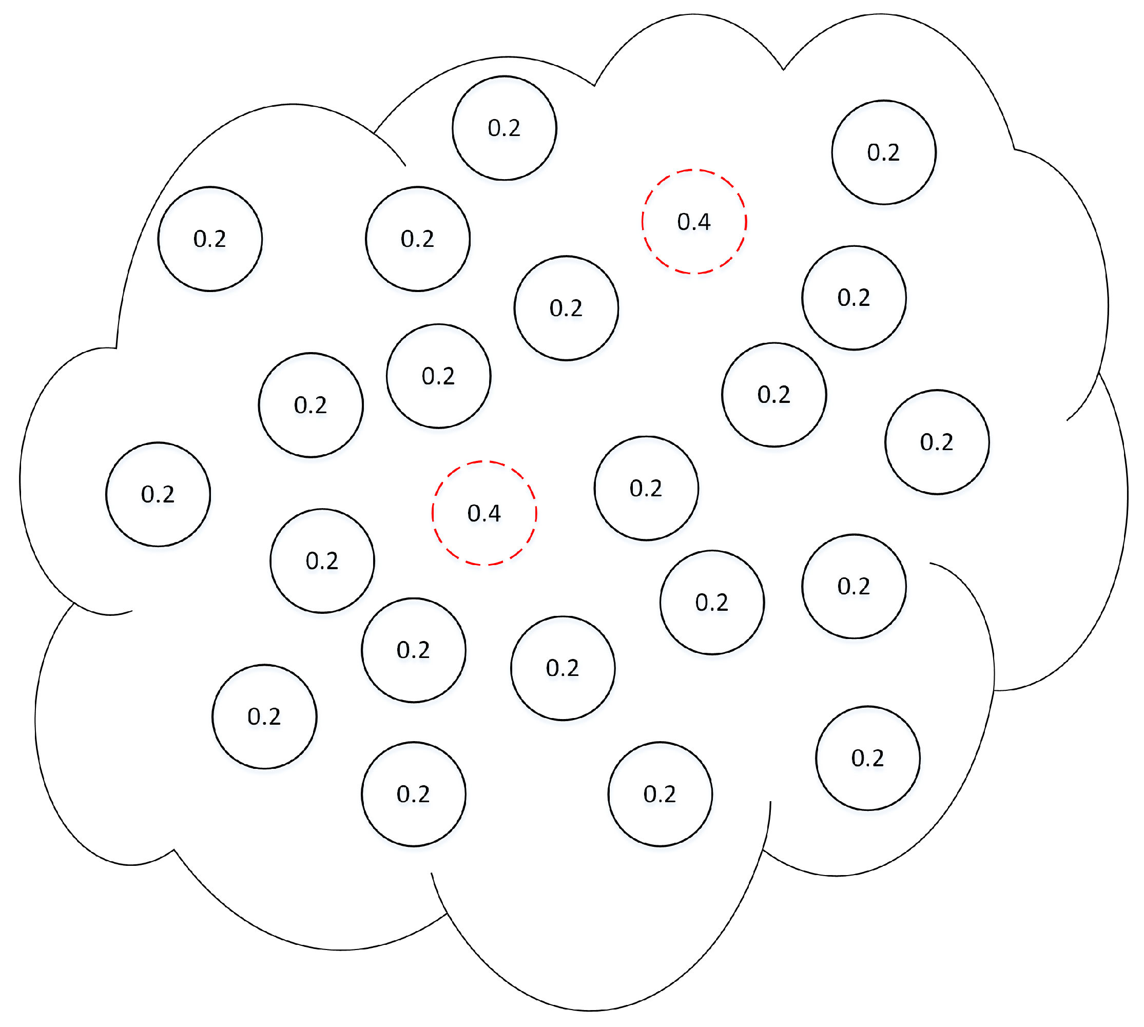
Rate Monitoring means that the adversary can differentiate between transmission rates of network nodes. If a node has a higher transmission rate than other nodes, this node is easily detectable, e.g., the 0.4 transmission rate some nodes use in
Figure 9.
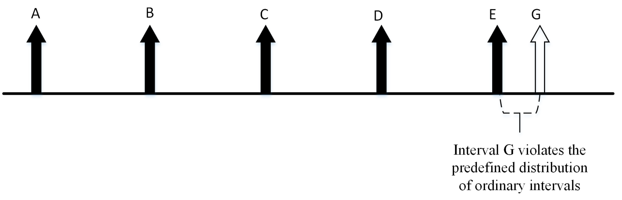
Time Correlation means that the adversary can distinguish the difference of transmission times between packets. For instance, in
Figure 10, interval G does not seem that it follows the same distribution of the other intervals. Therefore, if network nodes transmit packets using uniform distribution, and one of these nodes decided to transmit packets without using the uniform distribution, the adversary can easily differentiate between these packets.
Visualization means that the adversary has the ability to convert the sending/not-sending behavior of the network nodes into a binary image. This image can be analyzed to gain meaningful information about the real event.
Machine Learning means that the adversary can employ a classifier such as the neural network to analyze the traffic of the
WSN. Finally,
Statistical Methods mean that the adversary is able to perform a sophisticated statistical analysis.
7. Conclusions
In this work, we have provided a survey of the literature on dummy packets source anonymity techniques. Such techniques are very effective against global adversaries in WSNs. They out-perform other methods such as separate path routing, network location anonymization, and network coding. Further, the source anonymity problem has been discussed, and we present a detailed explanation of the most popular dummy techniques including their assumptions for the global adversary models. In addition, a comparison of all techniques has been provided to show the difference in terms of intervals, timers, random numbers, probability, clusters/grids/cells, proxies/filters, uniform/constant distribution, exponential distribution and Poisson distribution. Other surveys have not addressed such taxonomy in details. Another comparison for the global adversary models is also conducted. All models are compared to each other in terms of topology information, sink location, GPS/localization, interval distribution, rate monitoring, time correlation, visualization, machine learning, and statistical analysis. Some of the presented techniques are promising and have the potential for improvement. The main aim of the paper is to help those who are interested in the wireless sensor networks area choose a suitable algorithm that satisfies their applications’ demands by providing all the characteristics and assumptions of each technique in details. This will help them to make the right choice to get the maximum possible performance out of their applications. We did not cover all techniques that use dummy packets but we chose those which are mature, noble and advanced in performance. In the future, the dummy packet injections techniques can be expanded and improved by merging them with other methods such as network location anonymization to reduce the overhead of the dummy traffic, which is the main concern of the current techniques. The Internet of things (IoT) and WSN are both Machine-to-Machine (M2M) networks. IoT is a technology integrator for many already existing technologies such as embedded systems, sensing, data mining, cloud computing, etc. Furthermore, we can consider WSN as a part of the family of IoT depending on the scale of the application. Some of these algorithms/techniques/protocols could be used for IoT and would depend very much on the complexity of the IoT system on hand.


